1. Introduction
The emergence of microservices architecture as a popular approach to building software systems has led to a renewed interest in decomposing monolithic applications into microservices. The microservices architecture is characterized by the division of a software system into a set of small, independently deployable services that work together to provide the overall functionality of the system. The benefits of this approach, such as improved scalability, flexibility, and maintainability, have made it a popular choice for modern software systems.
Decomposing a monolithic application into microservices can be a challenging task, particularly when dealing with large and complex systems. One of the main challenges is identifying appropriate boundaries between microservices. In general, microservices should be loosely coupled, meaning that they should have minimal dependencies on other services. However, identifying the appropriate boundaries between microservices can be a difficult task, especially when the application is large and complex.
Several approaches have been proposed to address the challenge of microservices decomposition, including manual decomposition and automated techniques. Manual decomposition involves a human expert analyzing the application and identifying the appropriate boundaries between microservices. This approach can be time-consuming and error-prone, particularly when dealing with large and complex systems. Automated techniques, on the other hand, use algorithms to automatically identify the appropriate boundaries between microservices. However, these techniques often rely on heuristics and may not capture the complex dependencies between application components accurately.
In recent years, machine learning techniques have shown promise in addressing the challenges of microservices decomposition [
1]. In particular, graph neural networks [
2] and variational autoencoders [
3] have emerged as powerful tools for decomposing monolithic applications into microservices. Graph neural networks are a type of neural network that can operate on graph-structured data, such as the dependencies between application components. They are capable of capturing the complex dependencies between application components, which can be used to identify appropriate boundaries between microservices.
Variational autoencoders are a type of parametric generative model that can learn a low-dimensional representation of high-dimensional data. They have been used in various domains to learn representations of complex data, such as images and text. In the context of microservices decomposition, variational autoencoders can be used to learn a low-dimensional representation of the application components, which can be used to identify appropriate boundaries between microservices.
The objective is to decompose a monolithic application into microservices. However, this comes with its own set of challenges. During the decomposition, how do we know the right number of classes to have in a microservice? If the microservices are too coarse-grained, we have the same problems as with a monolithic application, and we do not really solve the issues of the monolithic application. On the other hand, if the microservices are too fine-grained, they will need to make multiple calls to perform even a basic task. In order to solve this, we need to find the right balance of classes in the microservices. In other words, we need to group only the classes that are highly dependent on each other in such a way that it also minimizes the communication between microservices. For the purpose of reducing communication between microservices, we also allow having the same class in multiple microservices. While this may be beneficial in minimizing inter-service communication, it brews another challenge of having to maintain the same class in multiple microservices. As we can see, there are a lot of trade-offs when it comes to microservices. So, there is no one best way to build a microservice. It depends on the scenario and the needs of the application. Our approach proposes a way to decompose a monolithic application into microservices that can be used as a guideline by practitioners to make an informed decision.
In this paper, we perform a case study of a method we previously proposed for decomposing a monolithic application into microservices using a variational autoencoder-based graph neural network [
1]. Our approach combines the strengths of both graph neural networks and variational autoencoders to suggest a way to decompose a monolithic application into microservices. The results of our approach can be used by developers and solution architects as a guideline to assist them in decomposing a monolithic application into microservices. In that paper, we test our approach against three mid-scale Spring Framework projects we created ourselves. In this paper, we demonstrate the effectiveness of our approach by performing a case study on the Food-To-Go application. We chose this application because it was created by a well-respected author, Chris Richardson. Furthermore, this project includes both a monolithic and a microservice version, providing us with a reliable source to validate our results. This project is part of the book
Microservices Patterns: With examples in Java [
4], written by Chris Richardson.
The remainder of the paper is organized as follows.
Section 2 gives a background of the major technologies used.
Section 3 reviews related work on microservices decomposition.
Section 4 provides an overview of our proposed approach, while
Section 5 presents our experiments and the results. We discuss our results in
Section 6.
Section 7 outlines the threats to validate, and
Section 8 concludes the paper. Finally, the list of abbreviations and additional figures can be found in Appendices
Appendix A and
Appendix B.
2. Background
We use graph neural networks (GNNs) to decompose monolithic applications into microservices. GNNs are a type of neural network that operates on graph structures [
2]. Graphs are a way of representing complex data structures that consist of nodes (or vertices) and edges (or connections) that connect them. Examples of graph-structured data include social networks, biological networks, atomic bounds, transportation networks, and citation networks.
Traditional neural networks are designed to operate on fixed-size input vectors or images, but GNNs can operate on graphs of arbitrary size and structure. The key idea behind GNNs is to learn a representation of each node in the graph that captures both its local structure and its global context. This representation can then be used to perform tasks such as node classification, graph classification, link prediction, and community detection.
GNNs typically consist of multiple layers, updating the node representations by aggregating information from their local neighbors. This aggregation process can be performed using different operations, such as sum, max, mean, or attention-based mechanisms. The final output of the GNN is a global representation of the entire graph, which can be used for downstream tasks.
GNNs have been applied to a wide range of real-world problems, such as predicting protein structures, recommending products to users, detecting fake news, and identifying communities in social networks. They have also been combined with other machine learning techniques, such as reinforcement learning, to solve more complex tasks.
Despite their success, GNNs still face challenges, such as scalability to large graphs, generalization to unseen graphs, and interpretability of the learned representations [
5]. Nevertheless, GNNs hold great promise for analyzing and modeling complex graph-structured data, and they are an active area of research in machine learning and artificial intelligence.
The other technology that we use in conjunction with GNNs is a variational autoencoder (VAE). VAE is a type of parametric generative deep neural network that learns the underlying structure of input data and generates new samples from that structure [
3]. It is a model that learns the data distribution in a compressed and structured latent space; the parameters of the learned distribution can then be used to generate new samples.
VAE is based on the concept of an autoencoder, that is, encoding and decoding. The encoding process maps the input data to a lower-dimensional latent space, while the decoding process maps the latent space representation back to the original input space. The network is trained to minimize the difference between the original and reconstructed input data. The reconstruction error is typically measured using the mean squared error (MSE) or binary cross-entropy loss.
VAE goes beyond a traditional autoencoder architecture by introducing a probabilistic approach to encoding. Instead of mapping each input to a single point in the latent space, VAE learns the parameters of a distribution that can map the input data to the latent space. This distribution is then used to sample points in the latent space for decoding, allowing new and diverse samples to be generated.
The training of a VAE involves maximizing the evidence lower bound (ELBO), which is a lower bound on the log-likelihood of the input data. The ELBO consists of two terms: the reconstruction loss, which measures the fidelity of the reconstructed data to the original input, and the KL divergence, which measures the difference between the learned latent distribution and a prior distribution [
3]. That is,
where
is the mean squared error (MSE) reconstruction loss,
are the original inputs,
are the reconstructed outputs, and
n is the number of samples. Then,
is the Kullback–Leibler (KL) divergence loss, where
and
are the mean and standard deviation of the
jth latent variable in the latent space, and
J is the dimensionality of the latent space. The KL divergence encourages the learned distribution to be close to a standard normal distribution, which makes sampling from the latent space easier.
VAE has been widely used in applications such as image generation, video generation, and speech generation. It has also been used in anomaly detection and data compression. VAE can generate new samples with high diversity and quality, making it a powerful tool for data generation and exploration.
In our approach, to incorporate structural information from the monolithic application, we apply a GNN on the constructed dependency graph. The GNN operates on a feature matrix derived from the static analysis data from the monolithic application, enabling each class node to aggregate information from its neighbors. This graph-based normalization enriches the feature representation of each class by capturing its contextual relationships within the application, laying the groundwork for more meaningful downstream embeddings. The normalized feature matrix obtained from the GNN is then fed into a VAE to generate compact and informative embedding vectors for each class. The VAE is trained to reconstruct the original input while ensuring that similar inputs result in similar latent representations. Additionally, a structural loss term is introduced to encourage embeddings of connected classes to remain close in the latent space. This results in an embedding matrix that captures both feature similarity and architectural proximity, which is later used for effective microservice clustering. These are described in more detail in the methodology section.
3. Related Works
Microservices decomposition is an active research area, and several approaches have been proposed to address the challenges associated with decomposing monolithic applications into microservices. In this section, we provide an overview of some of the related works that have been done in this area.
There have been several works that decompose a monolithic application into microservices. Chen et al. [
6] developed a dataflow-driven approach in 2017 to break down monolithic applications into microservices. Their method involved creating a manual Data Flow Diagram (DFD) and then combining the same operations with the same type of output data to create a decomposable DFD. From this, they identified potential microservices. In 2019, Taibi and Systa [
7] proposed a decomposition framework that used both static and dynamic analysis. Their six-step framework involved analyzing execution paths and frequency, removing circular dependencies, identifying options for decomposition, ranking them based on metrics, and selecting the best solution. However, their approach required expert input for some steps. In 2020, Krause-Glau et al. [
8] combined the bounded-context pattern of the domain-driven design with static and dynamic analysis to identify microservice boundaries. They divided the application into smaller bounded contexts based on domain analysis, partitioned the source code through static analysis, and used dynamic analysis for trace visualization. In 2021, Auer et al. [
9] introduced an assessment framework for migrating monolithic applications to microservices. They surveyed industry professionals to identify key metrics to consider before and after the transition, including functional stability, performance efficiency, reliability, maintainability, and cost.
Besides the purely software engineering approaches, there have also been various works that use machine learning to decompose a monolithic application into microservices. In 2021, IBM [
10] developed a tool called Mono2Micro for decomposing monolithic Java applications into microservices. The tool uses dynamic and static analysis techniques to generate a tree structure of the application’s classes and methods. Then, a hierarchical clustering algorithm is applied to partition the application into microservices. The tool also provides a web-based interface to visualize the application’s structure and microservice boundaries. The paper reports experiments with several open-source Java applications and shows that the Mono2Micro framework can effectively and efficiently decompose monolithic applications into microservices. Eski and Buzluca [
11] introduced an automatic extraction method that involves applying static analysis to an application and dynamic analysis to log files, followed by utilizing the agglomerative hierarchical algorithm to partition the application into microservices. They evaluated their approach by comparing its similarity with references implemented by experts. Abdullah et al. [
12] used URIs to partition a monolith application and applied the k-means algorithm to cluster them based on document sizes and response times. Then, they allocated a virtual machine (VM) for each microservice based on its document size and response time. They also proposed a simple auto-scaling algorithm for the VMs to dynamically scale out overloaded VMs. In 2020, Kalia et al. [
13] developed the Mono2Micro framework, which applies dynamic analysis to create a tree and static analysis to obtain information from the code, combines these results, and finally applies the hierarchical clustering algorithm to partition the application into microservices. Some researchers have started using graph neural networks (GNNs) to address this problem. Desai et al. [
14] converted a monolith application to a graph by treating each class as a node and each dependency as an edge. They applied the graph convolution network (GCN) [
15] on the generated graph, extracted an embedding vector for each node using an autoencoder, and clustered the nodes using the k-means algorithm based on their embedding vectors. In 2024, Sooksatra et al. [
16] expanded on our preliminary study [
1] by tuning the hyperparameters to optimize the decomposition of monolith to microservices. In 2024, Chy et al. [
17] also extended our preliminary study [
1] to optimize microservices. Mathai et al. [
18] proposed a similar approach to [
14] but used the heterogeneous graph neural network [
19] to handle multiple types of nodes and edges. Yedida et al. [
20] optimized the hyperparameters of existing machine learning-based monolith-to-microservices methods, using the work in [
14] as an example. In 2024, Trabelsi et al. [
21] also used the graph neural network to perform microservice decomposition. However, our approach differs from theirs because we use a variational autoencoder instead of the standard autoencoder. In 2025, Wei et al. [
22] proposed an approach to decompose microservices using graphs and K-means, unlike our C-means for clustering.
Moreover, several systematic mapping studies and literature reviews [
9,
23,
24,
25,
26,
27] have investigated the challenges and opportunities associated with decomposing monolithic systems into microservices. Collectively, these works report that while microservice migration offers notable benefits such as improved scalability, agility, and maintainability, it remains a technically complex and evolving area. Common motivations identified across these studies include the need to modernize legacy systems and address performance limitations, but persistent issues such as tightly coupled architectures, shared databases, and insufficient tool support continue to hinder migration efforts. Many approaches and frameworks have been proposed for microservice identification and decomposition, though most are still in early stages and often lack automation or standardized evaluation metrics. Some studies have introduced decision-support frameworks based on empirical evidence to guide organizations beyond intuition-based approaches.
The recent literature has also pointed to the potential of AI-assisted methods to automate aspects of the migration process. However, these approaches are still emerging, and challenges related to tool maturity, dataset availability, and the human factors of migration remain underexplored. Overall, while microservices adoption continues to grow, these studies emphasize that substantial gaps persist in automation, evaluation, and practical guidance.
4. Methodology
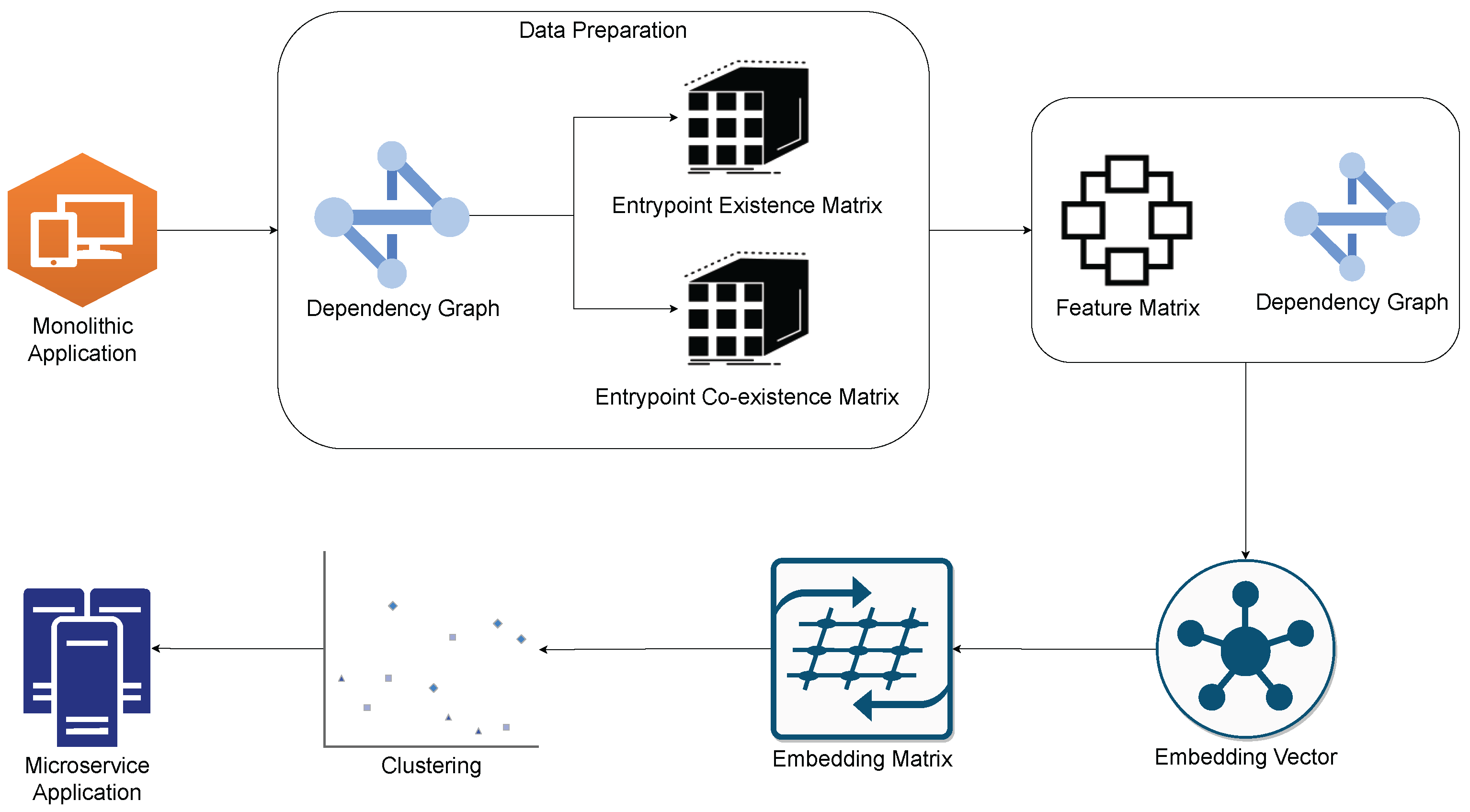
In this section, we describe the methodology that we use to decompose a monolithic application into microservices. The decomposition involves three major steps: Data pre-processing, embedding vector creation, and clustering. The process of preparing the data is a critical component of the microservices decomposition process. In order to achieve this, we use specialized tools to extract valuable information and construct a dependency graph based on the application. The dependency graph allows us to analyze the relationships and dependencies between various components of the application, which is necessary for effective decomposition.
Once we have constructed the dependency graph, we then move on to the next stage of the process, which involves generating more information from the graph and preprocessing it to create a feature matrix. This feature matrix contains important information that we can use to gain a better understanding of the application’s architecture and structure.
Having created the feature matrix, we then proceed to the embedding-vector creation stage. In this stage, we utilize a graph convolutional network to extract embedding vectors for each node in the graph. These embedding vectors capture the relevant information about each node, which we can then use to represent the node in a more concise and meaningful way.
Finally, in the clustering stage, we use the fuzzy C-means algorithm to determine the appropriate microservices. This algorithm is effective in identifying the optimal grouping of nodes into microservices based on their embedding vectors. Overall, this process allows us to effectively decompose a monolithic application into smaller, more manageable microservices. The overall flow of the system is shown in
Figure 1.
4.1. Data Pre-Processing
In order to decompose a monolithic application into microservices, we collect three different kinds of data: dependency graph, entrypoint existence matrix, and entrypoint co-existence matrix. The dependency graph is a matrix that shows all the classes that a particular class is dependent upon. In the context of this paper, an entrypoint refers to any class that initiates interaction with the application. In our case, entrypoints can be either an Application Programming Interface (API) endpoint or a message queue listener. The entrypoint existence matrix indicates which classes are present in at least one path initiated by a specific entrypoint. Let us denote the entrypoint existence matrix with E, then is set to one when class i is present in at least one path initiated by entrypoint j. Finally, the entrypoint co-existence matrix indicates the frequency with which two classes co-exist in the same paths initiated by the same entrypoints. Let us denote the co-existence matrix with Co, then refers to the number of paths where class i and class j co-exist in the same entrypoints. By collecting and utilizing these three types of data, we can effectively train the machine learning model to decompose the monolithic application into microservices.
For the purpose of collecting these data, we first generate an Abstract Syntax Tree (AST) of the monolithic application. After obtaining the AST of our code, we extract important information from it. To create the dependency graph for a specific class, we begin by retrieving a list of all the classes that it had imported. From this list, we then filter out any classes that were imported from external libraries and only include those classes that were within the project’s root package. This allows us to generate a more accurate and relevant dependency graph for the class in question. To generate the entrypoint existence matrix (
E) for a particular class
i, we use a depth-first search (DFS) algorithm on the dependency graph, starting from entrypoint
j as the root. During the DFS, if we encounter class
i at any point, we mark
as one. Similarly, to generate the entrypoint co-existence matrix (
Co), we perform DFS on the dependency graph and list all the paths that were initiated by the entrypoints. We then check for the existence of both class
i and class
j in these paths and set
to the number of paths where these classes co-exist. Finally, we create a feature matrix
as follows:
where ⊙ is the concatenation operation. Hence, from
, we know that the size of
is
where
C is the number of classes and
P is the set of entrypoints. Finally, using the graph convolutional network (GCN), we normalize
according to the adjacency classes in the graph by
where
,
I is the identity matrix,
is the degree diagonal matrix, and
.
4.2. Embedding-Vector Creation
After obtaining the dependency graph
A and feature matrix
X in the previous step, the aim is to generate an embedding matrix from
X that can be used to measure the similarity between two classes by using a similarity metric such as the
norm. A higher similarity score indicates that the two classes are more dependent. To create the embedding matrix, a variational autoencoder (VAE) is used because VAE is capable of arranging the latent vectors such that two comparable vectors represent two comparable inputs. In this step, X is considered an input of VAE, and the reconstruction of X is denoted by
. The feature matrix
Z is the latent space of VAE, where
and
l is the length of each embedding vector in
Z. The VAE is trained to generate a reconstruction of
X (
) that is as similar as possible to X. The loss function of the VAE consists of three parts. First, the reconstruction loss (i.e., the mean squared error) measures how close the output (
) is to the original input (
X), ensuring that the model can accurately recreate the input data without losing important information, similar to checking how clear a photocopy is compared to the original document. Second, the architecture loss measures how well the latent embeddings (
Z) preserve the relationships or connections between data points, as defined in the adjacency or structure matrix (
A), ensuring that data points with similar neighbors have similar representations, like making sure friends are positioned close together in a social network map. Lastly, the latent distribution loss, calculated using the Kullback–Leibler (KL) divergence, ensures that the latent embeddings follow a normal (Gaussian) distribution, which keeps the latent space organized and smooth, allowing meaningful sampling and generation of new data points, similar to keeping marbles evenly spread in a bowl so that picking any one of them represents the whole set. Overall, these three components work together to ensure accurate reconstruction, structural consistency, and organized latent representation in the VAE model. Hence, we can calculate the loss function of VAE as follows:
where
is the norm
,
n is the number of classes,
is the row
i of the matrix
X,
is the prior distribution of
Z where we assume it is the normal distribution (i.e.,
),
is the probability of
Z based on the input
X, and KL
is the KL divergence function between
Z and
. The definition of this KL function is
where
d is the latent dimension, and
and
are the mean and standard deviation of the
j-th latent dimension (
Z). In (
6), the first term is the reconstruction loss, the second term is the architecture loss, and the last term is the latent distribution loss. The
Z obtained from the VAE training with respect to the loss is used in the clustering phase.
4.3. Clustering
In this phase, we use the embedding matrix
Z that we obtained in the embedding-vector creation phase. We apply the fuzzy c-means algorithm on
Z to obtain the membership matrix
W, where
,
k is the number of microservices or clusters and
for every
i. The fuzzy c-means algorithm determines
W and a centroid matrix
, where
) by finding the local minimum of the following:
Here, the membership score () is a metric that represents the degree of association between a class j and a microservice i. The value of ranges from 0 to 1, inclusive, and it is computed for every class and microservice. After computing the membership score, we assign each class to a microservice if its score is higher than the maintainability threshold. The maintainability threshold is a predefined value that determines the minimum membership score a class must have to belong to a microservice. It is worth noting that if a class has membership scores higher than the threshold for two or more microservices, it can be assigned to multiple microservices. The ability to assign a class to multiple microservices is an important feature because it allows us to minimize communication between microservices. By duplicating a class in multiple microservices, the microservice does not have to make an API call to another microservice. However, the maintainability threshold must be carefully chosen to avoid too much redundancy, which can negatively impact performance and scalability.
5. Experiments and Results
5.1. Dataset
We chose to run our experiments on a popular project created by Chris Richardson, who is well-known in the field of Software Engineering, especially in the area of microservices. This project has both a monolithic and a microservice version. This allows us to compare the results of our approach against the existing microservice version to validate the results. This project is part of Chris Richardson’s book Microservices Patterns: With Examples in Java [
4]. Given the author’s authority in the field, we trust that the project adheres to sound microservice design principles. Additionally, at the time of this writing, the monolithic version of this project had 113 stars and 82 forks on GitHub, while the microservice version had over 3600 stars and 1400 forks, indicating its popularity and widespread use. Due to the reasons stated above, we are confident that testing our approach on this project will produce realistic and relevant results.
The monolithic version of the project is called
ftgo-monolith (
https://github.com/microservices-patterns/ftgo-monolith (accessed on 1 July 2025)) and was developed using Spring Framework. It comprises 89 classes and 5 entrypoints. The microservice version, named
ftgo-microservice (
https://github.com/microservices-patterns/ftgo-application (accessed on 1 July 2025)), was created by breaking down the monolith version into smaller services. However, additional features have been incorporated into the microservice version since then. There are a total of 7 microservices in the ftgo-microservice, all of which were implemented using the Spring Framework. It contains a total of 298 classes and 8 entrypoints. Using the dataset in its current form would give us inaccurate results. So, we pre-process the dataset to achieve the best results. To obtain the most accurate results, we only consider the classes that were common to both the monolithic and microservice versions. As a result of doing so, we end up with 55 unique classes and 3 entrypoints that are common in both the monolithic and the microservice versions. Also, it turns out that two of the microservices in the microservice version are built with completely new classes, so we remov those two microservices and end up with a total of five microservices.
5.2. Models
We decompose the monolithic application into microservices using three different approaches listed below:
It is worth noting that the architectures of AE and VAE are the same. That is, an encoder consists of an input layer, a 29-neuron dense layer, and a 14-neuron dense layer. The latent-space layer has only 2 neurons. We use 2 neurons for simplicity for visualization of other works. Also, our goal is to compare our approach to the other baselines that also use 2 neurons. Therefore, this number of neurons is not significant to our results. Then, a decoder includes a 4-neuron dense layer, an 8-neuron dense layer, a 16-neuron dense layer, and an output layer.
5.3. Results
In this section, we describe and compare the results that we obtain for all three models: AE-K, AE-C, and VAE-C. The
ftgo-microservice have five microservices:
ftgo-order-service, ftgo-restaurant-service, ftgo-consumer-service,
ftgo-kitchen-service, and
ftgo-delivery-service. Since the
ftgo-microservice has five microservices, all three models are also configured to produce five microservices. After running the experiments with all three models, we obtain the decomposition of the monolith to microservices in JSON format. Even though the models produced five microservices, we do not know which microservice corresponds with which service in the
ftgo-microservice. In order to map this, we loop through all five services of the
ftgo-microservice and compare them to all five produced by the models. We then pair the services with the highest number of matching classes. After this, we calculate the total match percentage by using the following equation:
where
M is the total match percentage,
X is the total number of common classes, and
T is the total number of classes in the
ftgo-microservice.
Table 1 shows the match percentage that we obtained for each of the three models.
Table 2 shows the percentage of classes from the
ftgo-microservice that are missing in the decomposed microservice. Finally,
Table 3 shows the number of classes that are added in the decomposed microservice that are not present in the
ftgo-microservice.
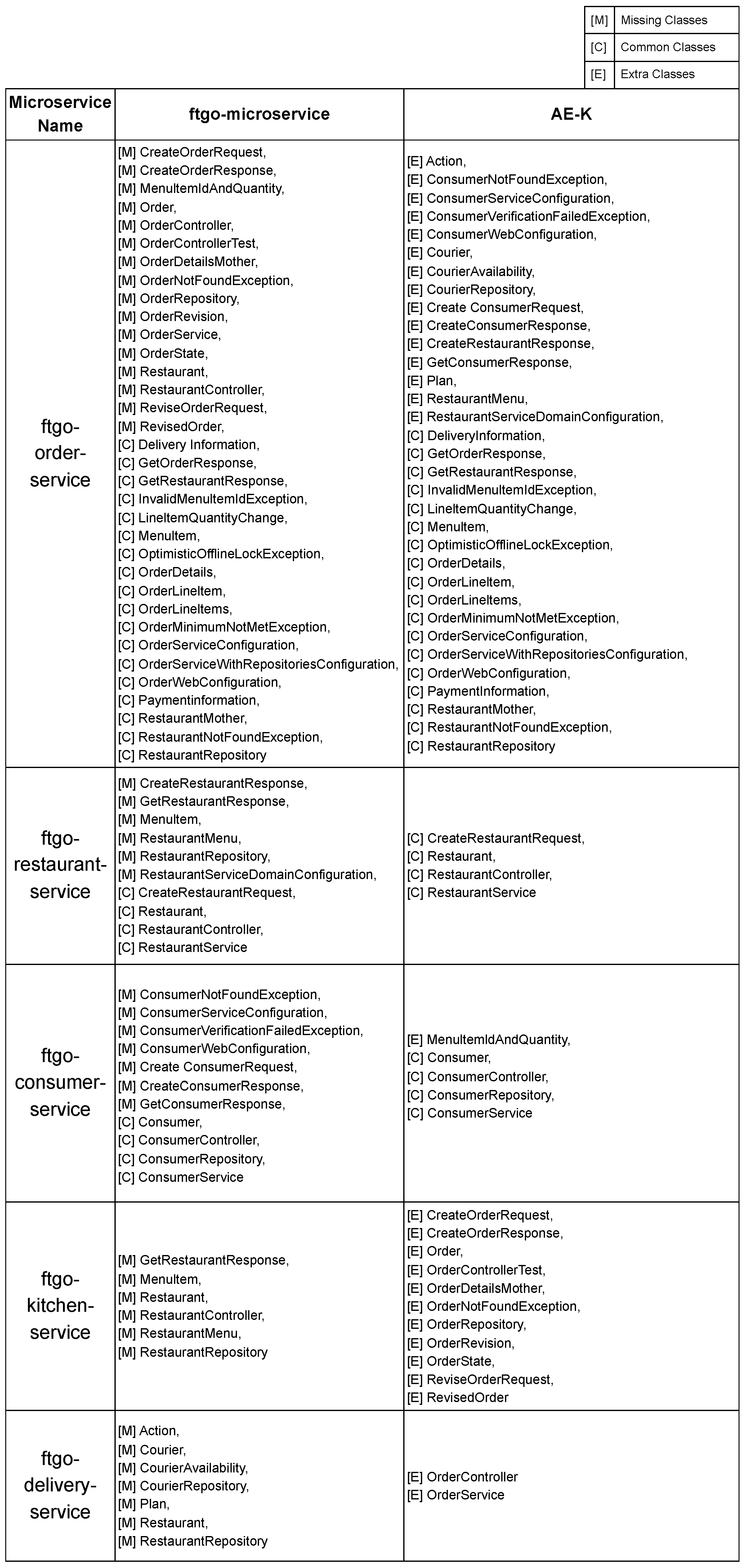
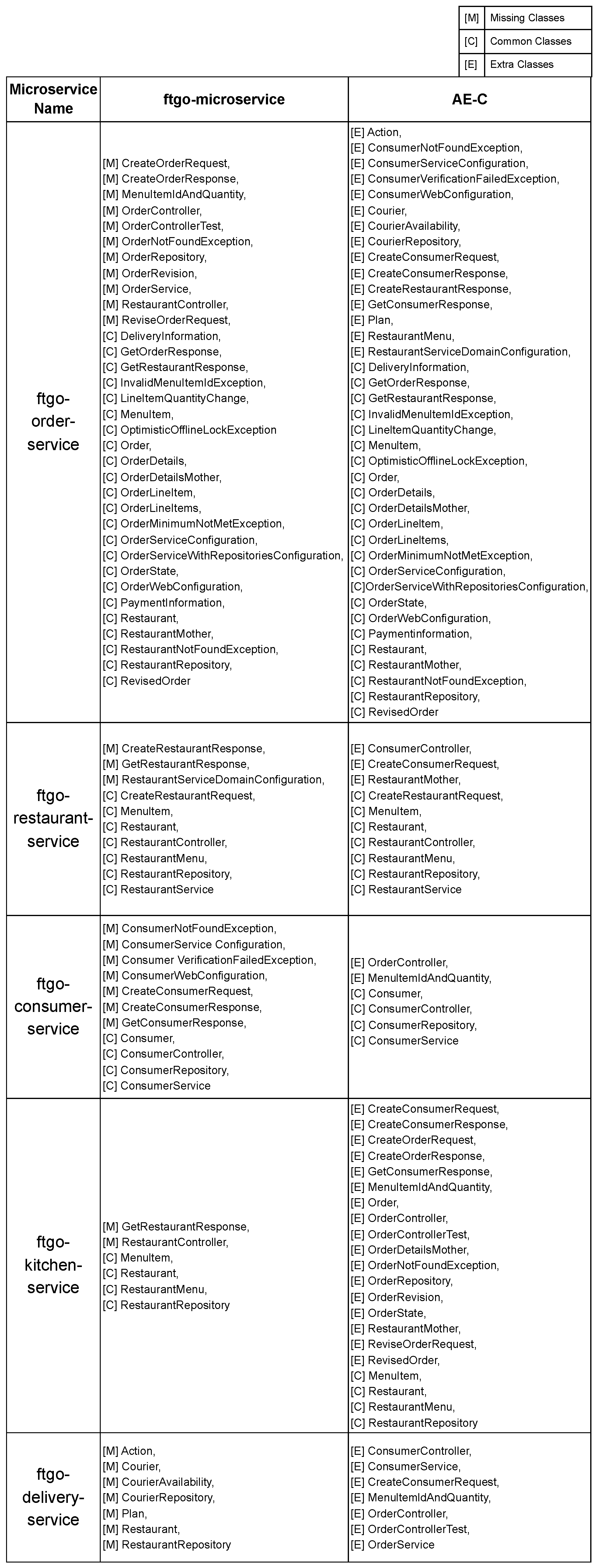
The detailed results of all the common, missing, and extra classes for AE-K can be found in Appendix
Figure A1, AE-C in Appendix
Figure A2, and VAE-C in Appendix
Figure A3. In these tables, we show the original classes in each service in the
ftgo-microservice and the decomposition predicted by the three models. The common classes between
ftgo-microservice and the decomposition are highlighted in green, the classes in
ftgo-microservice that are missing in the decomposition are highlighted in red, and the additional classes in the decomposition that are not in
ftgo-microservice are highlighted in blue.
6. Discussion
As we can see from
Table 1, AE-K performs the poorest with 38.24% match with the
ftgo-microservice. This outcome can be attributed to the utilization of the K-means algorithm in this approach. In the K-means algorithm, the assignment is hard, which means a particular class can only belong to a single microservice. Due to this, there are no duplicate classes in the decomposed microservice. However, if we observe the classes in the
ftgo-microservice, we can see that it has duplicate classes in many services. This inability to assign a class to multiple microservices causes a lot of discrepancy between the
ftgo-microservice and the results of AE-K, resulting in a lower percentage match. With a match percentage of 55.88% with the
ftgo-microservice, the AE-C performs better than the AE-K. This is because this model uses the C-means algorithm to cluster the classes. The C-means algorithm considers the fuzziness of data point assignments. It assumes that a data point can have varying degrees of membership in multiple clusters. Due to this, a particular class may be assigned to more than one microservice, allowing duplicates in the microservice. The VAE-C performs the best with a match percentage of 73.53% with the
ftgo-microservice. This is mainly because of two reasons. Similar to AE-C, VAE-C also uses the C-means algorithm to cluster the classes, allowing duplicates in the microservice. The other reason is that we are using a variational autoencoder in this approach. VAEs create a more structured and meaningful latent space compared to traditional autoencoders. While standard autoencoders simply compress data into a latent vector without any constraint on how that space is organized, VAEs enforce the latent representations to follow a known probability distribution—typically a multivariate standard normal distribution. This regularization forces the model to place similar data points close to each other in the latent space, leading to smoother transitions and better clustering of classes. As a result, the latent space learned by a VAE is more informative and interpretable. Distances between points in this space carry semantic meaning, making operations like interpolation, sampling, and visualization more reliable.
If we observe
Table 3, we can see that AE-K assigns the least number of extra classes that were not present in the
ftgo-microservice. This can again be attributed to the fact that AE-K does not allow the duplication of classes. Hence, it only has a limited number of classes to assign, and once a class is assigned to a microservice, it cannot be assigned to another microservice. On the other hand, both AE-C and VAE-C have higher values for extra classes than AE-K. This is because both AE-C and VAE-C allow the duplication of classes. A higher number of duplicate classes can either be a good or a bad thing, depending on the situation. Having more duplicate classes can help minimize inter-service communication, but it can also lead to increased maintenance overhead if those duplicate classes are edited frequently. Likewise, having too few duplicate classes can lead to significant inter-service communication while reducing the overhead of maintaining duplicate classes. Choosing the right balance depends on the needs of the system. Additionally, both the AE-C and VAE-C can be configured to vary the level of duplication by changing the maintainability threshold. As stated in the previous sections, the maintainability threshold is a predefined value that determines the minimum membership score a class must have to belong to a microservice. A higher maintainability threshold would reduce the number of duplicate classes, while a lower maintainability threshold would increase the number of duplicate classes.
In our previous research [
1], we demonstrated that our model, VAE-C, was highly effective at decomposing small-scale monolithic applications into microservices. In this current study, we take it a step further by applying VAE-C to a mid-sized monolithic system—and the results are just as promising. Specifically, VAE-C is able to match 70.53% of the classes with those in the actual microservice benchmark. This level of alignment suggests that the model not only scales well but also maintains its ability to identify meaningful service boundaries even as the system grows in complexity. Of course, a 70.53% match rate is not perfect, but that is expected. There is no universally correct way to decompose a monolith—different architects may arrive at different microservice designs even when working from the same set of requirements. Microservice boundaries often reflect architectural preferences, domain understanding, and performance goals, all of which can vary from one team to another. So, while VAE-C may not replicate every human-made decision, the high overlap demonstrates that it captures many of the key patterns and functional separations that define good microservice design.
Overall, these findings reinforce our belief that VAE-C offers a practical and scalable approach for guiding the decomposition of monolithic systems. It can serve not only as a tool for automation but also as a decision-support framework for architects exploring different decomposition strategies.
7. Threats to Validity
Our approach to training a variational autoencoder on dependency graphs may not work well on noisy data. This is because we only train our variational autoencoder on clean data, and noisy data may contain incorrect information about the dependency graph, entrypoint existence matrix, and entrypoint co-existence matrix. Additionally, the hyperparameters for training an autoencoder or variational autoencoder are diverse, and we only use the hyperparameters that resulted in the best outcomes in our experiments. There may be other hyperparameters that we did not test that could outperform our hyperparameters.
Our approach cannot be used for applications that do not have the structures of classes and entrypoints. This is because we need this information as training data to train our models.
8. Conclusions and Future Work
In this paper, we presented an approach to decomposing a monolithic application into microservices using a variational autoencoder (VAE)-based graph neural network (GNN) in combination with the C-means clustering algorithm (VAE-C). To train our model, we conducted static analysis on the monolith and extracted three types of data: the dependency graph, the entrypoint existence matrix, and the entrypoint co-existence matrix. We evaluated our approach using the well-established monolith-to-microservice benchmark application developed by Chris Richardson, which provides both monolithic and microservice implementations.
We compared our VAE-C method against two baselines: Autoencoder with K-means clustering (AE-K) and Autoencoder with C-means clustering (AE-C). Our results showed that VAE-C achieved the highest match with the benchmark microservice architecture—correctly assigning 73.53% of the classes. In comparison, AE-C achieved 55.88% and AE-K significantly lagged behind at 38.24%. These findings highlight two important advantages: first, the C-means clustering algorithm’s ability to assign a class to multiple services aligns more closely with real-world microservice patterns, where functional overlaps are common. Second, the latent space learned by the VAE captures richer, more semantically meaningful relationships between classes than a traditional autoencoder, enabling better clustering outcomes.
Overall, our study demonstrates that VAE-C is not just an academically sound approach—it is also a practical tool that software architects can use as a guideline when decomposing monolithic systems. Unlike purely manual methods, which are time-consuming and prone to bias, our method offers a data-driven starting point that reveals potential service boundaries. It can assist practitioners in identifying cohesive groupings of classes that are candidates for microservices, while still allowing room for human judgment and domain-specific refinement.
While the results are promising, we recognize that further improvements are possible. Incorporating dynamic analysis could provide deeper insights into runtime interactions and dependencies. Additionally, mining version control history—particularly the frequency of file modifications—could help inform smarter duplication strategies. For example, frequently modified classes duplicated across services could increase maintenance costs, whereas infrequently modified ones may be duplicated with minimal overhead and reduced coupling. Another promising direction is to optimize clustering by incorporating bounded contexts from domain-driven design (DDD), which could improve the semantic alignment of the resulting microservices. We leave these enhancements as directions for future research.


 ,
, 

