Abstract
In an era marked by the rapid growth of the Internet of Things (IoT), network security has become increasingly critical. Traditional Intrusion Detection Systems, particularly signature-based methods, struggle to identify evolving cyber threats such as Advanced Persistent Threats (APTs)and zero-day attacks. Such threats or attacks go undetected with supervised machine-learning methods. In this paper, we apply K-means clustering, an unsupervised clustering technique, to a newly created modern network attack dataset, UWF-ZeekDataFall22. Since this dataset contains labeled Zeek logs, the dataset was de-labeled before using this data for K-means clustering. The labeled data, however, was used in the evaluation phase, to determine the attack clusters post-clustering. In order to identify APTs as well as zero-day attack clusters, three different labeling heuristics were evaluated to determine the attack clusters. To address the challenges faced by Big Data, the Big Data framework, that is, Apache Spark and PySpark, were used for our development environment. In addition, the uniqueness of this work is also in using connection-based features. Using connection-based features, an in-depth study is done to determine the effect of the number of clusters, seeds, as well as features, for each of the different labeling heuristics. If the objective is to detect every single attack, the results indicate that 325 clusters with a seed of 200, using an optimal set of features, would be able to correctly place 99% of attacks.
1. Introduction and Background
In an increasingly digital world where there is constant data transfer from device to device, and with nearly 75 billion devices predicted to be connected to the Internet of Things (IoT) network by 2025 [1], network security is now as important as ever. Intrusion Detection Systems (IDS) are essential tools used to monitor network traffic for malicious patterns that could be potential attacks. Traditional IDS techniques, however, face significant challenges in detecting new and evolving attacks as they rely heavily on labeled training data and already existing attack patterns. Signature-based detection are traditional methods that compare network traffic against known attack patterns, or signatures. They work by matching audit events against well-known patterns of attacks [2]. The issue with such signature-based network intrusion detection systems is that they can be ineffective against newer malware threats that become increasingly complex and sophisticated. Such methods are known as supervised methods since they require data to be labeled before data can be used for detection. Thus, unknown attacks may go undetected because there are no labeled examples of them in the training data.
The development of efficient and modern methods for IDS is critical. Historically, failures in intrusion detection have brought severe consequences to companies and users, including financial losses, reputational damage, and data breaches. These limitations in IDSs highlight the need for unsupervised or even semi-supervised techniques, which do not rely totally on labeled data or existing attack patterns. Attacks like Advanced Persistent Threats (APTs) and zero-day exploits, for example, continuously change their behavior and signatures, making them difficult to detect using signature-based approaches. Clustering allows IDSs to identify unusual data in network traffic without having prior knowledge of attack signatures, making it useful in today’s cybersecurity landscape.
Most machine learning algorithms work well with labeled data. But real-world data is naturally unlabeled. Moreover, there is also a major time commitment as well as computational cost involved in labeling data. Clustering is an unsupervised machine learning technique widely and efficiently used to characterize and group large unlabeled datasets, ranging from financial to medical data and beyond. In this work, our objective is to use clustering to characterize or group large network traffic data into attack vs. non-attack data. Since the objective of any good clustering algorithm would be to have high intra-cluster similarity and low inter-cluster similarity [3], the goal in developing our clusters would be to develop groups of attack clusters and groups of non-attack clusters, each group having similar characteristics within themselves while having low attack cluster and non-attack cluster similarity, that is, low inter-cluster similarity.
Hence, in this study, the aim is to achieve intrusion detection utilizing K-means clustering, a popular clustering algorithm [3], widely implemented due to its low computational complexity [3]. K-means clustering, a distance-based clustering algorithm [4], is applied to a modern newly-created network attack dataset, UWF-ZeekDataFall22 [5]. Finding the ideal number of clusters using K-means clustering can be challenging, especially in large datasets [3], hence the uniqueness of this paper is in presenting three different labeling heuristics to find the ideal number of clusters using connection-based features. After K-means clustering is performed using unlabeled data, the labels from the labeled dataset are used to determine which cluster points were attacks and this is used to predict the class of the cluster. K-means clustering has also not been used on connection-based data in any previous work.
Though this dataset contains labeled Zeek logs [6], this dataset was used as an unlabeled dataset, that is, the labeled Zeek logs from UWF-ZeekDataFall22 [5] were de-labeled before using this data for this study. This study will help us identify the parameters needed to apply K-means clustering efficiently to an unlabeled MITRE ATT&CK-based Zeek log dataset, creating attack and non-attack clusters. Zeek logs were created using Zeek [6], a network security monitor that captures and analyzes network traffic.
Due to the size of this dataset, UWF-ZeekDataFall22 [5], and to address the challenges faced when using Big Data, the Big Data framework, that is, Apache Spark [7] and PySpark [8] using Jupyter Notebooks [9], was used for our development environment. VMware was used to simulate virtualized environments, and the experiments were conducted on personal computers equipped with multi-core processors to handle the computational demands. Hence, leveraging the clustering capabilities of K-means in a Big Data environment, this study aims to enhance the detection of cyber threats and provide a robust, automated approach to cybersecurity monitoring using unlabeled data. An in-depth study is done, using our three different labeling heuristics, to find the ideal number of clusters, seed value, as well as features, needed to group attacks and non-attacks in UWF-ZeekDataFall22 [5]. A visualization of the attack/non-attack data is also performed using PCA.
The rest of the paper is organized as follows. The next sub-section, Background, presents the background needed to understand this study; Section 2 presents the related works, that is works related to clustering in the context of network intrusion data; Section 3 describes the UWF-ZeekDataFall22 dataset; Section 4 presents the experimental setup; Section 5 presents the K-means clustering results and discussion; Section 6 presents the limitations of this study; Section 7 presents the conclusions and Section 8 presents the future works.
Background
In order to categorize cyber attacks and understand the different techniques and stages at which attacks take place, for example, adversary behavior, tactical approaches, and systematic malicious actions, a modern cybersecurity behavioral framework, the MITRE Adversarial Tactics, Techniques, and Common Knowledge (ATT&CK) framework [10] was used for creating the UWF-ZeekDataFall22 dataset. Created in 2013 and maintained by the MITRE Corporation, a non-profit organization, ATT&CK is a “globally accessible knowledge base of adversary tactics and techniques based on real-world observations” [10]. This framework is based on certain core components: tactics, techniques, procedures, and mitigations. ATT&CK contains 14 types of tactics, which contain many techniques and sub-techniques under them. As attacks evolve and emerge, the framework is regularly updated, containing over 200 techniques and 435 sub-techniques as of its latest 2024 update [11]. The UWF-ZeekDataFall22 parquet files [5] contain various types of attacks and their occurrences, over several dates in the fall semester of 2022. The attacks are categorized under 12 different tactics, as presented in Table 1.

Table 1.
MITRE ATT&CK Tactics included in UWF-ZeekDataFall22 dataset [12].
While a number of studies have employed the KDD-Cup99 dataset to analyze IDSs, our paper differs from others through the use of a more recent dataset. The survey paper, by Bohara et al. (2020) [13], confirms that KDDCup99 remains the most commonly used dataset for anomaly detection in IDS due to its volume, as it features millions of training and test datasets containing 41 features and 24 types of attacks. However, it must be noted that the KDD-Cup ‘99 dataset comprises data from almost 25 years ago. In contrast, our research leverages Zeek data from Fall 2022, which is a significantly more contemporary dataset in comparison to the KDD Cup 1999 dataset that most other studies use in clustering algorithms. The UWF-ZeekDataFall22 [5] dataset captures a variety of attack types, including Reconnaissance, Credential Access, Execution, and others listed in Table 1. All of these align with the MITRE ATT&CK framework, thus providing a comprehensive representation of current attack tactics. Our use of the UWF-ZeekDataFall22 dataset overcomes another drawback of the KDD Cup ‘99 dataset, which is known for containing a large number of duplicate records in the training and test sets, thus complicating the categorization of network traffic with redundant records [14].
This study can be considered semi-supervised as it uses unlabeled data to build clusters and labeled data only to determine which clusters contain attacks. The labeled data was used for comparison and verification of results only.
2. Related Works
In the field of IDS, numerous studies have explored the application of clustering techniques for anomaly detection, including hierarchical, grid-based, density-based, distribution-based, as well as centroid-based clustering, such as the K-means technique used in this paper. In addition to K-means, other methods such as K-medoids, linear regression, and other hybrid algorithms that combine multiple methods have also been studied to improve the accuracy of anomaly detection. In this section, we first present works that have been done using K-means clustering for IDSs, and then we look at works that have been done in other related areas like partition-based and hybrid-clustering and K-medoids. Finally, we look at works that have been done using the UWF-ZeekDataFall22 dataset and then address the gap this paper seeks to fill.
2.1. Enhanced K-Means Clustering
Yassin et al. (2013) [15] and Sharma et al. (2012) [16] explore enhanced versions of K-means clustering as they analyze the combination of K-means (unsupervised) with Naive Bayes classification (supervised). By combining supervised and unsupervised methods, the authors aimed to accurately categorize data before clustering. Although both papers analyzed K-means clustering (KMC) with Naive Bayes Classification (NBC), the prior paper reported better results, claiming that the enhanced KMC + NBC algorithm “substantially increased the accuracy and detection rate up to 99% and 98.8% respectively, while keeping the false alarm reduced to 2.2%” [15]. By contrast, Sharma et al. (2012) [16] found that the enhanced algorithm allowed for higher detection but generated more false alarms. The difference in results could be attributed to the fact that Yassin, et al. (2013) [15] use the ISCX 2012 dataset, while Sharma et al. (2012) [16] implement the KDD-Cup99 dataset. As discussed earlier, while this dataset contains millions of instances of training and test data, it has high redundancy and therefore contains only a small percent of unique data points. 78% of the training set and 75% of the test set are duplicated, and due to its high redundancy, only a small percent of the KDD-Cup99 dataset has unique data points [14]. In contrast, while the ISCX dataset is smaller, it proves to be better at evaluating IDSs as it is much newer than the KDD-Cup99 dataset and thus contains more recent, realistic attack data. Because a key limitation of K-means is its high sensitivity to the initially chosen centroids, several studies have attempted to address this limitation of K-means by combining it with optimization algorithms.
Xiao et al. (2006) [17] introduces Particle Swarm Optimization (PSO), a classification technique used to find optimal solutions through dimensionality reduction, inspired by the social behavior of swarms. When integrated alongside K-means, PSO enhances the accuracy of IDS by improving centroid selection and accelerating convergence speed. Tested on the KDD-Cup99 dataset, the PSO-KM combination demonstrated improved global search capability and IDS performance. However, it still failed to overcome a disadvantage of K-means: the dependency on the number of clusters.
2.2. Enhanced Partition-Based and Hybrid Clustering (Grid-Based + Density-Based)
Tomlin et al. (2016) [18] explored a clustering approach with industrial intrusion detection data from an attack in 2010 that was able to bypass security measures and cause infections on SCADA systems through thumb drives and network shares. This study applied partition-based clustering methods of fuzzy c-means (FCM) and K-means clustering to group data into tight, distinct clusters. The focus of this paper was to enhance detection rates by introducing a fuzzy inference system to identify anomaly signatures. The initial results of this system were poor due to its inability to detect attacks that appear normal; however, the reduction of clusters and analysis of data structures created a more effective approach for evaluating attacks on SCADA systems.
Similar to Tomlin et al. (2016) [18], Siraj et al. (2009) [19] uses a hybrid clustering model aimed at optimizing alert management in network intrusion detection systems (NIDS). The authors used K-means clustering combined with Expectation-Maximization (EM), and FCM with unit range (IUR) and principal component analysis (PCA) to reduce alert redundancy and false positives. The utilization of the Intrusion Detection Message Exchange Format allowed data preprocessing, with EM particularly effective for sorting data into models based on local maximum likelihood estimates. The results of this study showed the significance of alert correlation and the benefits of integrating multiple clustering techniques to improve the efficiency and accuracy of network intrusion detection. However, because one of the main components of this algorithm is preprocessing to label the data, it can not only have high computational costs, but it is also a supervised method, making it not useful against evolving attacks.
Portnoy (2000) [20] and Leung and Leckie (2005) [21] address these limitations by employing unsupervised techniques in IDS. Portnoy (2000) [20] uses purely unsupervised clustering-based anomaly detection to detect intrusions, with K-means used to detect deviations from normal network traffic patterns in the KDD-Cup99 dataset. The algorithm demonstrated good performance, with a high detection rate (40–55%) and a low false positive rate of 1.3–2.3%. However, the authors note that the performance of their algorithm is highly dependent on the training set used, with different datasets leading to significantly varied results. Their reliance on the outdated and redundant KDD-Cup99 data for optimal performance limits the applicability of their approach to modern and evolving network traffic environments. Leung and Leckie (2005) [21] propose a new grid-based and density-based algorithm called fpMAFIA, also designed to address limitations of supervised methods like misuse detection, which rely on labeled data and cause high labeling costs. To mitigate this, Leung and Leckie (2005) [21] also employed unsupervised anomaly detection, leveraging existing normal data from the KDD-Cup99 dataset to detect new intrusions based on any deviation from it. Although fpMAFIA showed a high detection rate while reducing computational costs, it also had a high false positive rate, and further research is needed to improve its accuracy.
Another paper that aims to optimize alert management is Fatma and Mohamed (2013) [22], which uses a two-stage technique in order to improve the accuracy of an IDS and utilizes the DARPA 1999 dataset instead of the KDD-Cup99. The first stage classifies the generated alerts based on some similar features to form partitions of alerts using a self-organizing map (SOM) with the K-means algorithm and Neural-Gas with the fuzzy c-means algorithm. The second stage uses three approaches, SOM, support vector machine (SVM), and decision trees in order to classify the meta-alerts created in the first stage into two clusters: true alarms and false ones. It is a famous alert correlation technique that maximizes the degree of similarity between objects in the same cluster and minimizes it between clusters. Next, it classifies based on the similarity of some selected features (timestamp, source, and destination IP addresses), so that alerts in the same partition are more similar to one another than they are to alerts in other partitions. Thus, the administrator will face a manageable set of alarms since all the closest ones are merged together and constitute one attack scenario. The results show that SVM provides the best performance since it has the best detection rate.
2.3. Centroid-Based K-Means Clustering
Most of the previously mentioned papers utilize either K-means or FCM techniques. Ranjan and Sahoo (2014) [23] introduce K-medoid clustering, comparing it to FCM, KMC, and Y-means clustering (YMC). Unlike K-means, which calculates the centroid as the average of all data points in a cluster, K-medoids use actual data points as centroids. This method is more robust to noise and outliers as it avoids relying on the mean, which can be heavily influenced by outliers. Using the KDD-Cup99 dataset, this study demonstrated that the K-medoids approach performed significantly better in intrusion detection than the other three methods: KMC, FCM, and YMC. Despite achieving a high detection rate and fewer false negatives, this algorithm has certain limitations. The authors suggest that future research could focus on improving efficiency to further enhance detection accuracy.
Another study by Tian and Jianwen (2009) [24] claims that K-means is not a “globally optimal solution” due to its high computational cost when working with large datasets since it calculates the distance between the data object and the center of each cluster each time it iterates. Similar to the PSO-KM optimization in Xiao et al. (2006) [17], this paper proposes a modified K-medoids method by combining it with the improved triangle trilateral relations theorem, which can lead to better detection of abnormal behavior while reducing false positives. The K-medoids method uses a data point in the cluster instead of the mean, and the triangle theorem reduces the distance computation time. The results show that this proposed algorithm effectively separates attack data from normal data, all while reducing computation time and obtaining a very high fault detection rate and a low false drop rate. However, like Xiao et al. (2006) [17], this algorithm fails to address the dependence of centroid-based clustering on the initially chosen centroid. Simply choosing a different initial central point deeply influences the result.
2.4. Works Using UWF-ZeekDataFall22
To date, the works on UWF-ZeekDataFall22 [5] have used classification algorithms. Bagui et al. (2023) [25] utilized UWF-ZeekDataFall22 to classify attack tactics such as reconnaissance, discovery, and resource development using supervised machine learning algorithms, including decision trees, random forests, and gradient-boosting trees. Their study demonstrated that binary classification models, particularly decision trees and random forests, performed better in classifying these tactics with high accuracy. Moomtaheen et al. (2024) [26] utilized Extended Isolation Forest to classify the UWF-ZeekDataFall22 dataset and Krebs et al. (2024) [27] utilized multi-class support vector machines to classify UWF-ZeekDataFall22.
2.5. Addressing the Gap
While all the previous studies have employed various methods including enhancing centroid-based clustering, grid and density-based clustering, and the optimization of clustering methods, our paper highlights its uniqueness in several ways. First, through its use of the UWF-ZeekDataFall22 dataset, which provides non-redundant, current, and relevant network traffic data rather than the widely used but 25-year-old KDD-Cup99 dataset that many of the above-mentioned studies employ. Second, in contrast to other works, this paper applies K-means clustering to detect evolving cyber threats without requiring labeled data. The labeled data is only used to compare the results. Since no prior knowledge of specific attacks is required, this makes our work more adaptable for real-time intrusion detection, allowing the detection of new and previously unknown attack patterns. Third, none of the previous works have focused on using just the connection-based features of network traffic for clustering.
3. Data Description: UWF-ZeekDataFall22
The dataset utilized for this research, UWF-ZeekDataFall22 [5,25], is a comprehensive network traffic dataset collected over a semester using Zeek [6], an open-source network traffic analyzer, and labeled as per the MITRE ATT&CK framework [10]. Zeek excels in high-speed, high-volume network monitoring and produces extensive logs capturing network activities across multiple protocols. The dataset was designed and generated to simulate real-world cyber-attacks.
3.1. Features in UWF-ZeekDataFall22
This dataset includes multiple files containing nominal, numeric, and object variables that provide a rich description of network events. Key fields in the dataset are as follows:
- Connection logs (conn): This provides detailed information about network connections, including source and destination IPs, ports, protocol type, connection state, and transferring data (bytes and packets);
- DNS logs: This provides information on DNS queries, including query types, response times, and whether requests were resolved;
- DHCP logs: This does data linking, for example, linking IP addresses with MAC addresses, assisting in identifying hostnames, and tracking device connections;
- Mission logs: This is used to map and label network events with MITRE ATT&CK tactics and techniques based on simulated attack scenarios.
- Each of these files plays a crucial role in identifying various phases of network interactions, ranging from routine traffic to suspicious or malicious behaviors.
3.2. Data Distribution and Size
The dataset consists of network traffic, that is, 42.8 GB of Zeek logs collected across 81 subnets. The data was transferred daily from a Security Onion Virtual Machine to a Big Data platform, utilizing Hadoop’s distributed file system (HDFS) for storage and analysis. This distributed approach allows for efficient handling of the high volume of network data generated [28].
A significant feature of this dataset is the balanced representation of attack and normal traffic:
- Non-malicious traffic: 350,339 records;
- Malicious traffic: 350,001 records.
These records were labeled according to the MITRE ATT&CK techniques, as presented in Table 1, enabling detailed analysis of adversary behaviors and attack phases such as reconnaissance, discovery, privilege escalation, and exfiltration.
3.3. Zeek and Its Role
Zeek (formerly Bro) [6] is a prominent tool used for collecting Zeek logs that provides a structured, detailed view of network traffic and is highly suitable for post-processing with external software. Zeek logs capture a wide range of protocol interactions, including TCP, UDP, and ICMP traffic, along with in-depth transaction logs like DNS requests and responses. Its versatility and ability to monitor large-scale network environments make it the optimal choice for collecting data in this experiment. Zeek’s output format is log files.
Key Features Collected
- Protocols: The dataset includes diverse protocol types such as TCP, UDP, and ICMP, with unique flows across thousands of IP addresses.
- Traffic details: Features like the number of bytes, packet counts, and connection states are meticulously logged, providing a comprehensive view of both normal and attack traffic.
- Network coverage: The dataset covers 254 unique source IP addresses and 4324 unique destination IP addresses.
- More details on the UWF-ZeekDataFall22 dataset are available at [5,25].
4. Experimental Setup
This section outlines the steps taken to apply the K-means clustering model to detect cyberattacks in the UWF-ZeekDataFall22 dataset. The workflow, as illustrated in Figure 1, involved preprocessing the data, creating column vectors, applying the K-means algorithm, labeling the clusters as attack or non-attack, and finally, comparing the actual attack/non-attack labels to evaluate the model’s performance.
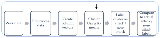
Figure 1.
Experimental Workflow.
4.1. Preprocessing
The main concept used in preprocessing was binning the data. This was done to reduce the number of discrete values as well as to group the data. Before we present the discussion on binning this data, we will present the features used for this study.
4.1.1. Features Used
Of the 23 features available in this dataset [5,25], the connection-based features, that is, connection state, the type of network protocol, duration of the connection, the number of bytes and packets transferred, and where the bytes and packets were transferred from, that is, the source and destination ports, were used. In short, 12 features were selected for this analysis: duration, the network protocol (proto), the connection state (conn_state), source and destination ports (src_port_zeek and dest_port_zeek respectively), the number of packets transferred (orig_pkts and orig_ip_bytes, and resp_pkts and resp_ip_bytes, which refer to origination packets and bytes and response packets and bytes, respectively) and missed_bytes. These features are briefly described next:
- duration—Duration of network connection
- proto—Network protocol (e.g., TCP, UDP, ICMP)
- conn_state—Connection state of network communication
- src_port_zeek—Source port in network communication
- dest_port_zeek—Destination port in network communication
- orig_pkts—Number of packets from originator
- resp_pkts—Response packet count
- orig_ip_bytes—Bytes sent from originator
- resp_ip_bytes—Bytes sent from responder
- orig_bytes—Total number of bytes from originator
- resp_bytes—Total number of bytes from responder
- missed_bytes—Bytes missed in transmission, representative of packet loss
4.1.2. Binning
In Big Data, since analysis can become computationally intensive and expensive, binning was used to group the variables. In particular, binning was used to group the network ports, connection state, and network protocols.
Network Ports
Dest_port_zeek and src_port_zeek represent the ports involved in network communication. As per [6,25,29], to simplify the range of potential port numbers, the ports were categorized into:
- Bin 0: Null or missing values
- Bin 1: System Ports (0–1023)
- Bin 2: User/Registered Ports (1024–49,151)
- Bin 3: Dynamic/Private Ports (49,152–65,535)
- Bin 4: Out-of-range or unclassified ports
Connection State
The connection state, conn_state, feature describes the state of a network connection. The various connection states were grouped into distinct bins, as follows:
- Bin 0: RSTH (Reset with acknowledgment)
- Bin 1: SF (Normal establishment and termination)
- Bin 2: S0 (Connection attempt with no reply)
- Bin 3: OTH (Other conditions)
- Bin 4: REJ (Connection attempt rejected)
- Bin 5: RSTO (Reset received with no acknowledgment)
- Bin 6: RSTR (Reset sent in response to a connection attempt)
- Bin 7: SH (Synchronized half-open connection)
- Bin 8: S2 (Partially established connection)
- Bin 9: S1 (Connection attempt with no reply)
- Bin 10: SHR (Synchronized half-open connection response)
Protocol
To categorize the different network protocols in the network traffic data, the protocol (proto) column was used. This column was separated into four separate bins based on the type of their network protocol, as shown below:
- Bin 0: TCP (Transmission Control Protocol)
- Bin 1: UDP (User Datagram Protocol)
- Bin 2: ICMP (Internet Control Message Protocol)
- Bin 3: All other protocols
4.2. Creating Column Vectors
After binning, all the selected features were assembled into a single vector using VectorAssembler in PySpark. This step allowed for the handling of multiple feature columns as a single input for the scaling process. To ensure consistent feature scaling and improve clustering performance, StandardScaler from PySpark [8] was used to normalize the selected features. StandardScaler works by scaling each feature by dividing it by its standard deviation, ensuring that all features have a comparable scale while preserving their distributions. The resulting scaled features were used as input for the K-means algorithm, improving clustering accuracy by preventing features with larger magnitudes from dominating the model.
4.3. K-Means Clustering
K-means clustering is a popular unsupervised machine learning algorithm designed to group data into clusters based on similarity [4]. Being an unsupervised algorithm, K-means does not need pre-labeled data, hence, though UWF-ZeekDataFall22 [5] is labeled, the labeling was removed for the K-means clustering in this study. The goal of K-means clustering is to partition the data into k distinct clusters, with each data point assigned to the cluster whose centroid (mean) is the closest.
4.3.1. Steps in the K-Means Clustering Algorithm
- Choose the number of clusters, k.
- Randomly select k centroids as starting points for the clusters.
- Assign each data point to the nearest centroid using the Euclidean distance.
- Recalculate the centroids by averaging the data points in each cluster.
- Repeat the process until the centroids stabilize and do not change.
The Euclidean distance was used in K-means to measure the distance between data points and centroids, to determine the cluster assignments. The formula for the Euclidean distance is [4]:
4.3.2. Seed Selection and Impact on Clustering
The selection of initial centroids, or seeds, plays a crucial role in determining the final clusters. Different seeds may cause the algorithm to converge on different cluster formations, sometimes leading to suboptimal solutions known as local minima. By experimenting with various seed values, these risks were minimized, and better clustering was attained. The K-means clustering equation [4], which calculates clusters based on the distance between data points and centroids, is presented next.
4.4. Clustering in Cyber-Attack Detection
After K-means clustering was performed, the labels from the labeled dataset were used to determine which cluster points were attacks. A new column, “Prediction”, was added to the DataFrame, to hold this data, and predict the class of the cluster.
4.5. Evaluation
Labeled attack data was used to evaluate the effectiveness of our unsupervised K-means clustering model. The labels, which indicate whether or not an attack occurred, were applied only during the evaluation phase to calculate the key performance metrics: accuracy, precision, recall, F1 score, AUC, and Confusion Matrix. These metrics provided a benchmark to prove that our clustering approach successfully distinguished between normal and attack data. That is, actual labels from the ‘label’ column were used to classify clusters as attack clusters or normal clusters. Once classified, a ‘prediction’ column was created, where all data points within the attack clusters were labeled as attacks, while those in normal clusters were labeled as normal data. Then the classification was evaluated by comparing the ‘prediction’ column against the actual labels, computing accuracy, precision, recall, etc. Hence, by comparing the clusters produced by K-means with the known attack labels, we were able to verify the model’s accuracy in identifying cyber threats.
The key statistical metrics are defined as:
- Accuracy offers an overall assessment of the model’s performance, representing the proportion of total correct predictions.
- Precision indicates the accuracy of the model’s positive predictions, reflecting how often these predictions are correct.
- Recall measures the model’s ability to capture all actual positive instances, showing its sensitivity to detecting attacks.
- F1 Score balances precision and recall, offering a single metric that reflects the model’s effectiveness in handling positive cases.
- AUC evaluates the model’s ability to distinguish between positive and negative cases.
- The confusion matrix provides a summary of the model’s correct and incorrect predictions for both classes, highlighting where the model succeeded and where it faltered.
5. K-Means Clustering Results and Discussion
This section presents the results and evaluation of our K-means clustering approach for cyber attack detection. The focus is on the three different labeling heuristics applied to the clusters, each yielding distinct results in terms of detection performance and false positives. Though the metrics and labeling approaches form the core of our analysis, the number of clusters, ideal seed value, and set of features that influenced the model’s success has to be determined first. Computational times (in seconds) were also recorded. A discussion of how these factors were fine-tuned and how they contributed to the final outcomes is also presented. A visual representation of the clusters is presented in the later part of this section. Since the results are presented for one run, the final sub-sections of this section present an analysis of the clustering stability and analysis of the distribution of data points across clusters.
5.1. Assessing Labeling Heuristics
Although our dataset, UWF-ZeekDataFall22, has several different types of attacks, as shown in Table 1, this clustering is performed on the attack versus non-attack data. That is, the analysis is not at the level of the attack, but whether a data point is an attack or not. Hence, after K-means clustering was performed on the data, the labels from the labeled dataset were used to determine which cluster points were attacks. A new column, “Prediction,” was added to the DataFrame to hold the data and predict the class of the cluster. Experimentation was performed with three distinct heuristics for labeling attack clusters:
- First Method: Clusters with At Least One Attack labeled as Attack Clusters
- Second Method: Clusters with at Least 25% Attack Data labeled as Attack Clusters
- Third Method: Clusters with at Least 50% Attack Data labeled as Attack Clusters
For each labeling method, the twelve previously mentioned connection-based features were used: duration, proto, conn_state, src_port_zeek, dest_port_zeek, orig_pkts, resp_pkts, orig_ip_bytes, resp_ip_bytes, orig_bytes, resp_bytes, and missed_bytes.
The threshold of 1, 25%, and 50% were selected to explore the trade-offs between high recall and low false positives when labeling clusters. The threshold of 1 assumes that a single attack in a cluster should raise concern, following the principle of maximum sensitivity, often applied in early-stage detection within the cyber kill chain framework. The 25% and 50% thresholds reflect increasing confidence in the cluster’s identity as primarily malicious, corresponding to mid-stage and late-stage actions within the MITRE ATT&CK lifecycle such as lateral movement or exfiltration. These thresholds also simulate differing tolerance levels in real-world intrusion detection, ranging from aggressive (1 single attack) to conservative (50%) strategies. Future work could include an adaptive threshold model based on the specific attack class or tactic.
5.2. Finding the Ideal Number of Clusters
The number of clusters in K-means clustering plays a crucial role in defining how well attack data is separated from normal traffic, especially in large datasets [3]. To determine the optimal number of clusters, values ranging from 2 to 350 for the First Method and values ranging from 2 to 400 for the Second and Third methods were used, evaluating their impact on accuracy, precision, recall, F1 score, and AUC. The following subsections analyze the results obtained from each labeling heuristic, detailing how performance varied as the number of clusters increased. Since results from multiple runs demonstrated stability when keeping all the configurations the same, we reported representative runs for each configuration. The results are presented in Table 2, Table 3 and Table 4.
Table 2.
Clusters with at least one Attack.
Table 3.
Clusters with at least 25% Attack Data.
Table 4.
Clusters with at least 50% Attack Data.
5.2.1. First Method: Clusters with at Least One Attack as Attack Clusters
In the first method, every cluster containing at least one attack was labeled as an attack cluster. Table 2 presents the results of the runs for clusters with at least one attack. A seed of 1 was used and though runs were done for all clusters between 2 and 350, only results for 2, 10, 50, 100, 200, 300, and 350 clusters are presented. Since the results were showing a downward after 300, the runs were stopped at 350.
Analysis of the results for the First Method:
- Performance with 2 clusters
- ○
- Since one cluster contained most of the attack points and the other cluster contained a mix of attack and normal data, both clusters were labeled as attack clusters.
- ○
- This resulted in an accuracy of only 49% and a very high number of false positives.
- Performance improvement with more clusters
- ○
- As the number of clusters increased, attacks and normal data were more effectively separated, leading to a gradual reduction in false positives.
- ○
- Though the computation time increased with the number of clusters, the best performance was observed at 300 clusters, where the model achieved 97.15% precision and 96.98% recall. These results are bolded in Table 2.
- ○
- Beyond 300 clusters, there was a slight decrease in performance, and computation time increased further, with 350 clusters resulting in a marginal drop in precision, possibly due to over-segmentation.
- Summary of the First Method
- ○
- This method is critical for scenarios where capturing all potential attacks is paramount as it prioritizes detecting every possible attack, even at the cost of a higher number of false positives.
5.2.2. Second Method: Clusters with at Least 25% Attack Data as Attack Clusters
In the second method, clusters were labeled as attack clusters if they contained at least 25% of attack data. Table 3 presents the results of the runs for clusters with at least 25% of attack data. In this set of runs, since a seed of 1 produced an error, a seed of 2 was used. At 400 clusters the results were very close to that of 300 clusters, but performance did not improve significantly, hence the runs were stopped at 400. Again, though runs were done for all clusters between 2 and 400, only results for 2, 10, 50, 100, 200, 300, and 400 clusters are presented.
Analysis of the results for the Second Method:
- Effectiveness from the beginning
- ○
- Since K-means naturally grouped 91.97% of the attacks into one cluster at two clusters, this method was able to label one cluster as an attack and the other as normal, leading to high precision from the start and a much lower number of false positives compared to the first method. Two clusters also had the lowest computation time.
- Best Performance at 300 Clusters
- ○
- Though the computation time went up quite a bit, the highest precision (98.74%) and recall (98.71%) were achieved at 300 clusters, where clusters were well-separated with minimal misclassification. These results are bolded in Table 3.
- ○
- At 400 clusters, the numbers were very close to those at 300, but performance did not improve significantly. While no significant increase in false positives was observed, there was no additional benefit in further segmentation at this stage. The computation time also increases with the number of clusters.
- Summary of the Second Method
- ○
- The Second Method had higher average accuracy, precision, recall, F1 score, and AUC than the First Method.
- ○
- Both the First and Second Methods had the best results at 300 clusters, but the computation time of the Second Method was slightly higher. In general, the average computation time was also higher with the second method.
5.2.3. Third Method: Clusters with at Least 50% Attack Data as Attack Clusters
In the third method, clusters were labeled as attack clusters only if 50% or more of the data points within the cluster were attacks. Table 4 presents the results for the clusters with at least 50% attack data. Since a seed of 1 and 2 were used in the previous runs respectively, a seed of 3 was used in this set of runs. At 350 clusters the results were very close to that of 300 clusters, but performance did not improve significantly, hence the runs were stopped at 350. Again, though all runs were done for all clusters between 2 and 350, only results for 2, 10, 50, 100, 200, 300, and 350 clusters are presented.
Analysis for the Third Method:
- Balanced Labeling Approach
- ○
- The 50% threshold ensured that only clusters predominantly composed of attack data were labeled as attacks, reducing false positives compared to the first method.
- Optimal Performance at 300 Clusters
- ○
- Though the computational time increased significantly at 300 clusters, this method achieved 98.64% precision and 98.61% recall. These best results are bolded in Table 4.
- ○
- Increasing clusters to 350 resulted in a slight performance drop, confirming that 300 clusters were the ideal choice for this method.
- Summary of the Third Method
- ○
- The second and third methods produced nearly identical results across all statistical measures.
- ○
- In terms of computation time, the computation time increased as the number of clusters increased. Also, in general, the third method had the highest average computation time of all three methods.
5.2.4. Overall Summary of the Three Heuristics
Figure 2 compares the accuracy across different numbers of clusters using the three labeling methods for cyber attack detection. All three heuristics had the best results at 300 clusters.
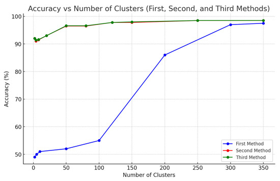
Figure 2.
Accuracy across the three methods.
Statistical results for the second and third methods were very similar, which is why, in Figure 2, the line representing the second method is nearly indistinguishable from the third method. Both approaches yielded high accuracy right from the start, even with just 2 clusters, achieving more than 92% accuracy in both cases. This demonstrates that both methods were highly effective at grouping the majority of attacks into the correct clusters, even with a minimal number of clusters. As the number of clusters increased, their performance remained strong and nearly identical, making both approaches excellent candidates for optimal performance. Ultimately, both methods converged to the same results, showing no significant difference in precision, recall, or accuracy across different cluster counts.
In terms of computational time, in all three methods, there was an increasing trend with the number of clusters, and a significant jump in computation time between 200 and 300 clusters. If computational time is of concern, 200 clusters can be selected in the Second and Third Methods, at the cost of an acceptable level of statistical compromise. In the First Method, however, 200 clusters have a significant drop in the statistical measures and would not be acceptable.
5.3. Finding the Ideal Seed Value
The seed value in K-means clustering determines the initial placement of centroids, which can influence how clusters are formed and hence the final clustering results. To assess this impact, since all three methods presented their best results at 300 clusters, various seed values were tested while keeping the number of clusters fixed at 300. The following subsections analyze the results obtained from each labeling method, detailing how performance varied with different seed values. The results are presented in Table 5, Table 6 and Table 7.
Table 5.
Performance Across Different Seed Values (First Method).
Table 6.
Performance Across Different Seed Values (Second Method).
Table 7.
Performance Across Different Seed Values (Third Method).
5.3.1. First Method: Clusters with at Least One Attack as Attack Clusters
Table 5 presents the results for runs with various seed values at 300 clusters, for clusters with at least one attack (First Method).
Analysis of the First Method:
- Impact of Seed Value on Clustering Stability
- ○
- Certain seed values led to significant fluctuations in precision and recall, while others resulted in stable and consistent clustering results.
- ○
- There was no definite pattern with regard to computational time.
- Best Performing Seed Values
- ○
- Seed values of 1, 10, 600, and 1000 produced very similar results, with precision and recall exceeding 97%.
- ○
- Amongst them, a seed of 600 yielded the highest overall precision (97.26%) and recall (97.10%), slightly outperforming other values. The computational time was also on the lower side at a seed value of 600. These best results are bolded in Table 5.
- Summary of First Method with Different Seed Values
- ○
- For the First method, a seed of 600 was selected as the ideal seed, as it consistently provided the most balanced and reliable performance. The computational time was also the second lowest, being second to a seed of 300 that had significantly lower statistical performance.
5.3.2. Second Method: Clusters with at Least 25% Attack Data as Attack Clusters
Table 6 presents the results for runs with various seed values at 300 clusters, for clusters with at least 25% attack data (Second Method).
Analysis of the Second Method:
- Impact of Seed Value on Clustering Performance
- ○
- When the attack data in the clusters were increased, on average, lower seed values produced higher results.
- ○
- On average, higher stability was observed compared to the first method, with less variability in results across different seed values.
- ○
- With regard to computational time, as in the First Method, there was no definite pattern.
- Best Performing Seed Values
- ○
- Strong performing seed values included 1, 2, 10, 200, and 100, all of which maintained precision and recall above 98.5%.
- ○
- Seed 200 provided the highest overall precision (98.75%) and recall (98.73%), making it the optimal seed for this labeling method. The computational time was also on the lower side. These best results are bolded in Table 6.
- Summary
- ○
- For attack clusters with at least 25% attack data, the seed of 200 was determined to be the most consistent and stable choice.
5.3.3. Third Method: Clusters with at Least 50% Attack Data as Attack Clusters
Table 7 presents the results for runs with various seed values at 300 clusters, for clusters with at least 50% attack data (Third Method).
Analysis of the Third Method:
- Impact of Seed Value on Clustering Performance
- ○
- Similar to the Second Method, this labeling approach produced stable results across different seed values.
- ○
- The clustering pattern was less sensitive to initialization, meaning that performance remained relatively consistent across multiple seeds.
- ○
- In terms of computational time, as in the First and Second Methods, there was no definite pattern.
- Best Performing Seed Values
- ○
- Seed values 1, 3, 10, 200, and 100 also showed strong performance, maintaining precision and recall above 98.5%. These results are very similar to the Second Method.
- ○
- Seed 200 produced the best results, with 98.76% precision and 98.73% recall. The computational time at a seed of 200 was also on the lower side. These best results are bolded in Table 7.
- Summary
- ○
- For clusters with more than 50% attack data, a seed of 200 was the most consistent and stable choice, similar to the 25% attack labeling method.
5.3.4. Overall Summary of the Three Methods for Finding the Ideal Seed Value
Figure 3 shows how the accuracy of K-means clustering varies with different random seed values, with the number of clusters fixed at 300 for all three labeling heuristics. The First Method (labeling clusters with at least one attack as attack clusters) shows high variability, with some seed values resulting in a significant drop in accuracy. In contrast, the Second and Third Methods (using 25% and 50% attack thresholds, respectively) are more stable across seed values. This highlights the importance of seed selection, especially in the First Method. In terms of computational time, the computational times of what were deemed the best results in each method (presented in bold in the respective tables, Table 5, Table 6 and Table 7) were relatively close for all three methods.
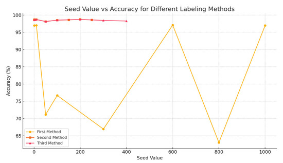
Figure 3.
Seed Value versus Accuracy for the Different Labeling Methods.
5.4. Finding the Ideal Number of Clusters with the Ideal Seed
After determining the optimal seed values for each K-means clustering method, we focused on identifying the best number of clusters to maximize detection accuracy and efficiency. The number of clusters directly influences how well attack and normal data are separated, impacting accuracy, precision, recall, F1 score, and AUC. The following subsections analyze the results obtained from each labeling method, detailing how performance varies across different numbers of clusters while using the ideal seed value for each method. The results are presented in Table 8, Table 9 and Table 10.
Table 8.
Performance Across Different Cluster Numbers (First Method).
Table 9.
Performance Across Different Cluster Numbers (Second Method).
Table 10.
Performance Across Different Cluster Numbers (Third Method).
5.4.1. First Method: Clusters with at Least One Attack as Attack Clusters
From the previous set of experiments, specifically Table 5, since the best results were obtained with a seed of 600 for clusters with at least one attack data record, the seed of 600 was used for the following set of experiments. And, looking back at Table 2 and Figure 2, the best results were obtained using clusters of 200 and higher, hence a starting point of 200 clusters was used for this experimentation.
Analysis of the First Method:
- Performance Improvement with More Clusters
- ○
- As the number of clusters increased, precision, recall, and accuracy improved, reaching a peak effectiveness at 350 clusters.
- ○
- At 350 clusters, the model achieved 97.58% precision and 97.45% recall, providing high accuracy while minimizing false positives.
- ○
- In terms of computational time, although the lower number of clusters (300 clusters or less) had lower computational times and the higher number of clusters (above 300 clusters) had higher computational times, there was no definite pattern.
- Optimal Number of Clusters
- ○
- At 400 clusters, a slight performance drop was observed, suggesting that further segmentation would not enhance classification.
- ○
- 350 clusters were chosen as the optimal cluster count for this method, balancing detection accuracy and computational efficiency.
- Summary
- ○
- A seed of 600 with 350 clusters will produce the best set of results for clusters with one attack. The best results are bolded in Table 8.
5.4.2. Second Method: Clusters with at Least 25% Attack Data as Attack Clusters
From the previous set of experiments, specifically Table 6, since the best results were obtained with a seed of 200 for clusters with at least 25% attack data, the seed of 200 was used for the following set of experiments. And, looking back at Table 3 and Figure 2, the best results were obtained using cluster sizes around 300, hence cluster sizes between 100 and 400 were tested for this experimentation.
Analysis of the Second Method:
- Performance Trends Across Cluster Counts
- ○
- Increasing the number of clusters improved detection accuracy, with precision and recall exceeding 98.7% beyond 200 clusters.
- ○
- In terms of computational time, although the lower number of clusters (250 clusters or less) had lower computational times and the higher number of clusters (above 250 clusters) had higher computational times, as in the First Method, there was no definite pattern.
- ○
- At 325 clusters, precision and recall reached 98.77% and 98.74% respectively, with no major changes after that, making 325 the optimal choice in terms of performance, but computational time was actually rather high for 325 clusters.
- Best Performing Cluster Count
- ○
- At 400 clusters, no additional gains were observed, reinforcing that 325 clusters were the ideal selection. Beyond this point, the model showed diminishing improvements, indicating that further increases in cluster numbers would not show significant performance benefits. Though computational time was high at 325 clusters, since there was no definite pattern in computational time, we are ignoring the aspect of computational time here.
- Summary
- ○
- A seed of 200 with 325 clusters will produce the best set of results for clusters with at least 25% attack data. The best results are bolded in Table 9.
5.4.3. Third Method: Clusters with at Least 50% Attack Data as Attack Clusters
From the previous set of experiments, specifically Table 7, since the best results were obtained with a seed of 200 for clusters with at least 50% attack data, the seed of 200 was used for the following set of experiments. And, looking back at Table 3 and Figure 2, the best results were obtained using cluster sizes around 300, hence cluster sizes between 100 and 400 were tested for this experimentation.
Analysis of the Third Method:
- Impact of Clustering on Performance Metrics
- ○
- Similar to the 25% labeling method (the Second Method), increasing clusters led to steady improvements in accuracy, precision and recall.
- ○
- At 325 clusters, precision and recall reached 98.77% and 98.74% respectively, with no significant improvements beyond this point, confirming 325 as the best balance between performance and efficiency.
- Optimal Number of Clusters
- ○
- At 400 clusters, no further improvements were observed, leading to the conclusion that 325 clusters are the most effective choice.
- Summary
- ○
- A seed of 200 with 325 clusters will produce the best set of results for clusters with at least 50% attack data. These best results are bolded in Table 10.
- ○
- The 25% and 50% labeling methods produced almost identical results, demonstrating consistent detection accuracy at higher cluster counts for clusters with greater than 25% attack data.
- ○
- In terms of computational time, as in the First and Second Methods, although the lower number of clusters (250 clusters or less) had lower computational times and the higher number of clusters (above 250 clusters) had higher computational times, there was no definite pattern.
5.4.4. Overall Summary of the Three Methods for the Ideal Number of Clusters with the Ideal Seed
Figure 4 presents the relationship between the number of clusters and accuracy for each labeling method, using the optimal seed values identified previously (600 for the first method, 200 for the second and third methods). The first method sees a gradual increase in accuracy with more clusters, peaking at 350 before slightly dropping. For the second and third methods, accuracy plateaus around 325 clusters, indicating that increasing clusters beyond this point does not significantly enhance performance. This figure helps establish the ideal number of clusters for each method to balance accuracy and computational cost.
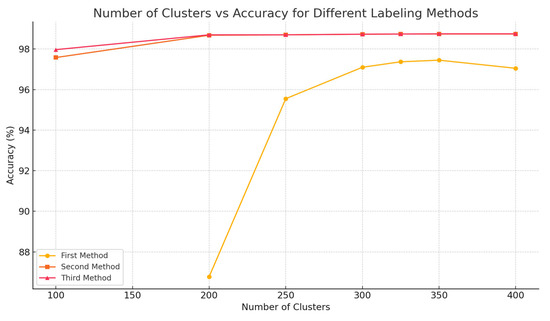
Figure 4.
Accuracy vs. Number of Clusters Using Optimal Seed Values.
5.5. Finding the Best Set of Features Within the Connection-Based Features
Feature selection plays a critical role in the performance of K-means clustering for detecting cyber attacks. The selection of relevant features impacts how well the model distinguishes between attack and normal data, influencing key performance metrics such as accuracy, precision, recall, F1 score, and AUC.
Though the 12 connection-based features were being used in the above experiments, the objective here is to determine if there is an optimal subset within the connection-based features. Hence, to determine the best subset of features, multiple feature subsets were tested under the three different labeling methods, using the optimal number of clusters and optimal seed values identified in previous sections, that is:
- For the First Method (At Least One Attack per Cluster): 350 clusters and a seed of 600
- For the Second Method (25% Attack Threshold): 325 clusters and a seed of 200
- For the Third Method (50% Attack Threshold): 325 clusters and a seed of 200
To assess the scalability of each feature subset, we estimated the memory usage of the scaled features, which encapsulates all normalized numeric features into a single vector, the actual data structure used in the K-means algorithm. The memory estimation was performed by multiplying the number of features per row by 8 bytes (the size of a 64-bit float) and summing across all rows using PySpark’s RDD API. The estimated memory usage for this column was approximately 64 MB, assuming 12 features per row and about 700,000 records.
5.5.1. First Method: Clusters with at Least One Attack as Attack Clusters
For this analysis, the same 12 initial connection-based features were considered: duration, resp_pkts, conn_state, proto, orig_ip_bytes, missed_bytes, orig_pkts, resp_ip_bytes, dest_port_zeek, orig_bytes, resp_bytes, and src_port_zeek. Set 1 was run with all these 12 connection-based features, as shown in Table 11. For the set 2 runs, the first feature, duration, was removed. If the statistical metrics, that is accuracy, precision, recall, etc. went down, that means that it negatively impacted the results, so this feature was considered important and was kept in the pool of features. If the results were the same or went up, then that feature was removed. In this manner, all the features were tested. The feature sets tested in the First Method are presented in Table 11. The corresponding performance evaluations for these feature sets are provided in Table 12. The best-performing cluster size of 350 and optimally performing seed value of 600, as shown in Table 8, were used to run the various feature set combinations.
Table 11.
Connection-based Features Used in the First Method.
Table 12.
Performance Across Different Feature Sets (First Method).
Analysis of the First Method:
- Impact of Feature Selection on Performance
- ○
- The choice of features significantly influenced the clustering results, affecting precision, recall, and overall detection accuracy.
- ○
- Some feature sets gave significantly better results, demonstrating that certain features are essential for effective attack detection.
- Best Performing Feature Sets
- ○
- Sets 9 and 11 yielded the highest precision (97.70%) and recall (97.59%), making these two sets the most effective feature combinations.
- ○
- Set 9 performed best when “missed_bytes” and “resp_ip_bytes” were excluded, suggesting that these attributes did not contribute significantly to distinguishing attack patterns in the First Method.
- ○
- Set 11 performed best when “missed_bytes”, “resp_ip_bytes”, and “orig_bytes” were excluded, suggesting that these attributes did not contribute significantly to distinguishing attack patterns in the First Method.
- Lower Performing Feature Sets
- ○
- Set 2 showed the weakest performance, with precision dropping to 80.13% and recall to 66.91%. The significant drop in performance on set 2 and 5 indicates that excluding “duration” and “proto” respectively negatively impacted the model’s ability to distinguish between attacks and normal traffic, hence these two features were actually kept.
- Summary
- ○
- For the First Method, set 11 (bolded) was determined to be the optimal feature set, as it provided the best balance of precision, recall, and overall accuracy and used the fewest features. Hence, the most significant connection-based features, using the First Method are: duration, proto, conn_state, src_port_zeek, dest_port_zeek, orig_pkts, orig_ip_bytes, resp_pkts, and resp_bytes. Also, set 11 had the lowest memory usage estimation.
5.5.2. Second Method: Clusters with at Least 25% Attack Data as Attack Clusters
For the Second Method, that is, for clusters with at least 25% attack data, set 1 contained the same original set of 12 connection-based features and the same techniques for keeping and removing features as was used in the First Method. The feature sets tested in the Second Method are presented in Table 13 and the corresponding performance evaluations for these feature sets are provided in Table 14. The best-performing cluster size of 325 and optimally performing seed value of 200, as shown in Table 9, were used to run the various feature set combinations.
Table 13.
Connection-based Features Used in the Second Method.
Table 14.
Performance Across Different Feature Sets (Second Method).
Analysis of the Second Method:
- Effectiveness of Feature Combinations
- ○
- Performance was less sensitive to feature selection compared to the First Method, but significant differences were still observed.
- ○
- Certain sets, such as set 13, provided consistently high results.
- Best Performing Feature Sets
- ○
- Set 13 achieved the highest precision (99.01%) and recall (99.00%), confirming its effectiveness for the Second Method.
- ○
- This feature set performed best when “missed_bytes”, “dest_port_zeek”, and “src_port_zeek” were excluded, indicating that removing these features improved the clustering efficiency.
- Lower Performing Feature Sets
- ○
- Sets 4 and 5 showed lower performance, highlighting the importance of conn_state and proto in maintaining high detection accuracy in the Second Method.
- Summary
- ○
- For the Second Method, set 13 (bolded) remained the best-performing feature set, producing stable and high-accuracy results. Hence, the best-performing connection-based features using the Second Method are: duration, resp_pkts, conn_state, proto, orig_ip_bytes, orig_pkts, resp_ip_bytes, orig_bytes, and resp_bytes. Also, set 13 had the lowest memory usage estimation.
5.5.3. Third Method: Clusters with at Least 50% Attack Data as Attack Clusters
For the Third Method, the same feature set combinations were used as were used for the Second Method, that is, Table 13. The respective performance evaluations are presented in Table 15. The best-performing cluster size of 325 and optimally performing seed value of 200, as shown in Table 10, were used to run the various feature set combinations.
Table 15.
Performance Across Different Feature Sets (Third Method).
Analysis of the Third Method:
- Feature Selection Stability
- ○
- Results were consistent with those observed in the Second Method, suggesting that this labeling approach was similarly robust across feature sets or selections.
- Best Performing Feature Sets
- ○
- Set 13 again provided the highest precision (99.01%) and recall (99.00%), confirming its stability as the best choice. The best results are bolded in Table 15.
- ○
- The best results were obtained when “missed_bytes”, “dest_port_zeek”, and “src_port_zeek” were excluded, similar to the Second Method.
- Lower Performing Feature Sets
- ○
- Sets 4 and 5 resulted in a significant drop in precision and recall, reinforcing the importance of conn_state and proto in clustering accuracy in the Third Method also.
- Summary
- ○
- For the Third Method also, set 13 (bolded) remained the best-performing feature set, producing stable and high-accuracy results. Hence, the best performing connection-based features using the Second and Third Methods are: duration, resp_pkts, conn_state, proto, orig_ip_bytes, orig_pkts, resp_ip_bytes, orig_bytes and resp_bytes. Also, set 13 had the lowest memory usage estimation.
5.5.4. Overall Summary of the Three Methods for Best Set of Features
Figure 5 compares the performance of different feature combinations (feature sets) on clustering accuracy for all three labeling methods using their respective ideal seed and cluster count configurations. Each feature set was created by iteratively removing one feature at a time and keeping only those that improved or maintained performance. The first method shows the highest sensitivity to feature selection, with performance fluctuating significantly. The second and third methods are more robust and share the same optimal feature set (set 13), which achieves the highest accuracy of 99%.
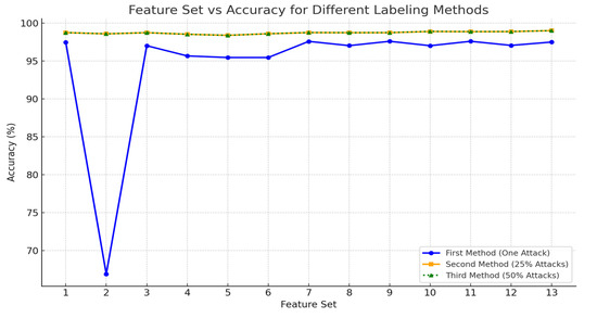
Figure 5.
Accuracy Across Different Feature Sets for Each Labeling Method.
5.5.5. Final Selection of the Best Connection-Based Feature Set
First Method (350 Clusters, Seed 600): Set 11 performed best without “missed_bytes”, “resp_ip_bytes”, and “orig_bytes”, with an accuracy of 97.59%. This set also had the lowest memory usage estimation.
Second and Third Methods (325 Clusters, Seed 200): Set 13 performed best when “missed_bytes”, “dest_port_zeek”, and “src_port_zeek” were excluded, and sets 4 and 5 performed the worst, reinforcing the importance of conn_state and proto. The best accuracy for set 13 for both methods was 99.00%. This set also had the lowest memory usage estimation.
This highlights that certain connection-based features did not contribute meaningfully to clustering performance in these labeling methods and were better removed to enhance model accuracy.
5.6. Visualizing the Clusters
To better understand how the attacks are distributed within the dataset and how well K-means clustering can separate them, Principal Component Analysis (PCA), a dimensionality reduction algorithm, was used to compress the feature space before graphing the data [4].
Using PCA, first the high-dimensional feature space was transformed into two principal components, allowing for a 2D visualization of the clusters. This approach preserved as much variance as possible while making it feasible to interpret the separation between normal and attack data points. By analyzing the PCA component loadings, the most significant features contributing to each principal component were identified. The primary contributor to the first principal component was identified as orig_ip_bytes and the second principal component was identified as proto. This indicates that the number of bytes sent from the original source (orig_ip_bytes) as well as protocol type (proto) played a major role in distinguishing between normal and attack traffic.
After applying PCA and using two principal components, the first step was to visualize the dataset without clustering, distinguishing attack data from normal data. As shown in Figure 6, the attack data (red) and normal data (blue) display a certain degree of overlap but also show some natural separation. This provided insight into the distribution of attacks before applying K-means clustering.
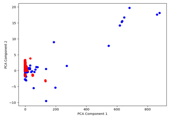
Figure 6.
Visualizing the Data Without Clustering (for two Principal Components).
After applying K-means clustering with two clusters (K = 2), the PCA model was able to separate over 92% of the attacks into one cluster. As seen in Figure 7, most attack data points are grouped into one cluster (also shown in Figure 6), confirming that a simple binary classification approach through clustering can provide significant separation between normal and attack data.
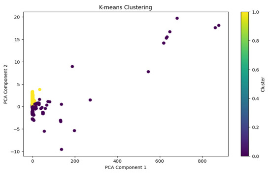
Figure 7.
K-means Clustering for k = 2 (for two Principal Components).
Increasing the number of clusters to three (K = 3) did not significantly improve the separation of attack data with two principal components. Figure 8 illustrates that, although an additional cluster was introduced, the separation of attacks remained relatively unchanged. This suggests that two clusters were already capturing most of the distinction between attack and normal data, and increasing to three clusters did not yield meaningful improvements.
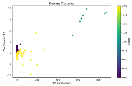
Figure 8.
K-means Clustering for k = 3 (for two Principal Components).
However, after increasing to fifty clusters (K = 50), for two principal components the point at which the model reached over 97% precision—the clustering pattern became significantly more fragmented. As shown in Figure 9, the attack and normal data points are now scattered across multiple small clusters. Though this makes it harder to interpret the visualization, it confirms that a higher number of clusters allows for finer-grained distinctions and improved precision.
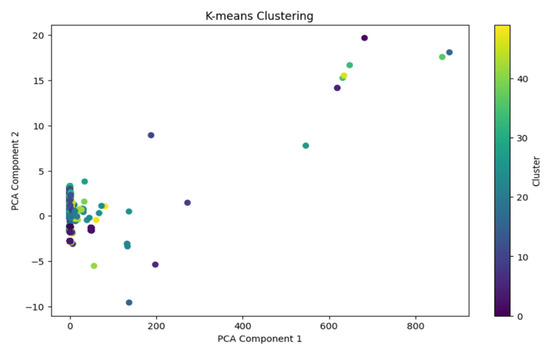
Figure 9.
K-means Clustering for k = 50 (for two Principal Components).
These results highlight that K-means clustering is effective in distinguishing attack traffic from normal traffic, even with as few as two clusters. The feature importance analysis using PCA further confirmed that orig_ip_bytes and proto were the strongest differentiators in the dataset, reinforcing the idea that network traffic volume and protocol types are key indicators in anomaly detection. However, as the number of clusters increases, interpretability becomes challenging, despite precision improvements. This analysis demonstrates how dimensionality reduction through PCA and clustering techniques can provide valuable insights for unsupervised anomaly detection in cybersecurity.
5.7. Cluster Size Distribution: An Analysis of the Distribution of Data Points Across Clusters
In analyzing the clustering results, a highly diverse distribution of cluster sizes was observed. Some clusters contained over 100,000 records, while others isolated individual data points. For example, using 325 clusters, the model yielded cluster sizes ranging from a minimum of 1 data point to a maximum of 139,063, with an average of 2251.90 data points per cluster. This variability was beneficial, as the formation of small, outlier-specific clusters improves the model’s precision by isolating anomalous behaviors. Since explicit distance-based outlier filtering was not applied and since the algorithm ensures that each point belongs to a cluster regardless of the distance from the center, several clusters consisted of single data points. There were no unallocated flows. These outliers or unique records were isolated into their own clusters, helping identify rare or unique behaviors, and improving the overall interpretability and robustness of the results. The presence of small clusters, alongside larger ones, reflects the natural heterogeneity of cyber traffic, strengthening the model’s ability to detect anomalies. Such dynamics highlight the adaptability of K-means in managing the heterogeneity present in network traffic data.
5.8. Clustering Stability Analysis
To assess the robustness of the clustering process to random initialization, a quantitative evaluation of clustering stability using the Adjusted Rand Index (ARI) [30] and Adjusted Mutual Information (AMI) [31] was used. ARI is used for evaluating the similarity between two clusters. It improves upon the Rand Index (RI) by correcting for chance—the chance that some data points can end up in the same cluster regardless of the underlying similarity. The RI uses two pieces of information, object pairs put together and object pairs assigned to different clusters in both partitions [32]. Generally, an ARI score closer to 1 indicates that the clustering algorithm was successful at capturing the underlying patterns in the data, and an ARI closer to zero indicates poor clustering performance [30].
AMI is calculated based on the mutual information between two clusters. It measures the amount of information that one cluster provides about the other. There is an adjustment for chance in AMI too. This adjustment for chance in AMI is achieved by subtracting the expected mutual information of two random clusters from the observed mutual information. AMI scores range from zero, which implies no mutual information, to one, which implies perfect mutual information. That is, higher scores imply greater similarity between clusters [31].
For our analysis, K-means clustering with k = 325 was used, since this yielded the best overall performance in our experiments, across 10 different random seeds. Pairwise comparisons of the resulting cluster assignments were computed to measure consistency across runs. The analysis yielded an average ARI of 0.9967 and an average AMI of 0.9917, with standard deviations of 0.0041 and 0.0025, respectively. These results indicate a high degree of stability and reproducibility in our clustering results.
6. Limitations of This Study
While this study presents strong results using K-means clustering for cyber threat detection, several practical considerations should be noted when applying these findings to real-world environments:
- Artificial Class Balance: The UWF-ZeekDataFall22 dataset used in this study contains a roughly 50/50 split between attack and normal data. This balanced distribution was designed to facilitate consistent metric evaluation and highlight the effects of different labeling strategies. However, in real-world network environments, attack data typically represents only a small fraction of overall traffic. As a result, further investigation is needed to validate the effectiveness of this approach in highly imbalanced scenarios where the rarity of attacks can impact both clustering and evaluation.
- Adaptive Thresholding: The use of 1, 25%, and 50% thresholds to label clusters as attack clusters reflects a range of detection sensitivities. While this provides useful comparisons between aggressive and conservative labeling strategies, these thresholds were arbitrarily chosen, based on some initial experimental results. An adaptive method based on cluster composition, risk levels, or known attack tactics may improve accuracy and generalizability. Further research is needed to develop adaptive thresholding mechanisms.
- Assumption of Cluster Geometry: The K-means algorithm assumes that clusters are spherical and separable by Euclidean distance. This assumption may not hold in complex network traffic where attack behaviors can form irregular or overlapping patterns. Alternative approaches such as DBSCAN, hierarchical clustering, or hybrid techniques could be explored to address this limitation.
7. Conclusions
This study demonstrated that applying K-means clustering to Zeek log data, specifically the UWF-ZeekDataFall22 dataset, can effectively group normal and malicious network activities. One of the key findings from our study was the impact of different heuristics for labeling attack clusters on the model’s performance. We experimented with three approaches: in the first method, a cluster was labeled as an attack cluster if it contained at least one attack; in the second, a cluster was labeled as an attack cluster if at least 25% of its data points were attacks; and in the third, a cluster was labeled as an attack cluster only if more than 50% of its data points were attacks. The results of the second and third methods were nearly identical, confirming that both approaches were highly effective in clustering attack data with minimal false positives. These methods consistently performed well, even at lower cluster counts, demonstrating their ability to detect cyber threats while maintaining accuracy. And, our clustering stability analysis confirmed this.
The first method, while generating more false positives, is particularly valuable for scenarios where capturing all potential attacks is the priority, as it ensures that no attack goes unnoticed. However, this method only produced strong results when the number of clusters was significantly increased. Unlike the second and third methods, which performed well even at lower cluster counts, the first method required a much higher number of clusters to achieve comparable performance.
We also found that the number of clusters (K) plays a crucial role in the effectiveness of the model. As the number of clusters increased, so did the model’s performance, underscoring the importance of selecting an appropriate K value to capture the complexities of the data. However, this also revealed a key trade-off: while increasing the number of clusters beyond 500, 700, and 1000 continued to improve results, it also significantly increased computation time and memory consumption. The more clusters used, the more computationally expensive the process becomes. For our experiments and real-world applications, our goal was to find a balance between achieving high accuracy and maintaining computational feasibility. As soon as the results stopped improving significantly, we determined that further increasing clusters would be impractical.
A significant aspect of our research involved exploring the importance of different sets of features for attack detection. Through experimentation, we found that the optimal feature set depends on the primary goal of the detection system. If the objective is to detect every single attack even at the cost of more false positives (First Method), then a broader feature set may be preferable. On the other hand, if the goal is to detect most attacks while minimizing false positives (Second and Third methods), a more selective feature set may be ideal. Our results showed that certain features, such as “duration”, “resp_pkts”, “conn_state”, “proto”, and “orig_ip_bytes”, played a critical role in improving detection accuracy. These features reflect key network and traffic properties that help distinguish between normal behavior and attack patterns. In contrast, omitting certain features led to a noticeable drop in performance, highlighting the importance of carefully selecting features based on the specific priorities of a cybersecurity system.
The process of determining the optimal seed value for K-means clustering was also significant. Each labeling method required a different ideal seed, highlighting the need for careful parameter tuning to achieve the best results.
Considering the computational feasibility of deploying K-means clustering on Big cybersecurity datasets, the full dataset, UWF-ZeekDataFall22, exceeded 200 GB, justifying the need for distributed processing, especially for memory-intensive steps like binning and feature engineering. Apache Spark’s in-memory distributed processing capabilities enabled the efficient processing of the entire pipeline, completing clustering tasks such that, our best-performing configuration, using the Second Method, at 325 clusters, seed = 200, and feature set 13 (which excluded missed_bytes, src_port_zeek, and dest_port_zeek), completed in under 14 s. This configuration produced a precision of 99.01%, recall of 99.00%, and overall accuracy of 99.00%, as shown in Table 14. This work highlights the impact of careful feature selection and parameter tuning in achieving high detection rates using unsupervised clustering methods.
8. Future Works
Future work will include empirical benchmarking against alternative algorithms such as Isolation Forest and DBSCAN. These comparisons will be conducted under uniform conditions and supported by statistical significance testing, which will further establish the comparative value of K-means in cyber threat detection scenarios.
Also, our model used 12 connection-based features derived from Zeek logs. While effective for structural analysis of network flows, incorporating additional features—such as payload analysis or time-based behavior—could further enhance the model’s ability to distinguish nuanced attack types.
Author Contributions
Conceptualization, S.S.B., G.C.S.D.C., D.M. and S.C.B.; methodology, S.S.B., G.C.S.D.C. and S.C.B.; software, G.C.S.D.C., A.M. and S.E.; validation, S.S.B., G.C.S.D.C., D.M. and S.C.B.; formal analysis, G.C.S.D.C., A.M. and S.E.; investigation, G.C.S.D.C., A.M. and S.E.; resources, S.S.B., D.M. and S.C.B.; data curation, S.S.B. and G.C.S.D.C.; writing—original draft preparation, S.S.B., G.C.S.D.C., A.M. and S.E.; writing—review and editing, S.S.B., D.M. and S.C.B.; visualization, G.C.S.D.C. and S.C.B.; supervision, S.S.B., D.M. and S.C.B.; project administration, S.S.B., D.M. and S.C.B.; funding acquisition, S.S.B., D.M. and S.C.B. All authors have read and agreed to the published version of the manuscript.
Funding
This research was funded by the 2021 NCAE-C-2002: Cyber Research Innovation Grant Program, Grant Number: H98230-21-1-0170. This research was also partially supported by the Askew Institute at the University of West Florida as well as the Office of Undergraduate Research at the University of West Florida.
Institutional Review Board Statement
Not applicable.
Informed Consent Statement
Not applicable.
Data Availability Statement
The data presented in this study are openly available in datasets.uw (datasets.uwf.edu).
Conflicts of Interest
The authors declare no conflict of interest.
References
- IoT Platforms: Enabling the Internet of Things. Available online: https://www.actuel-expert-comptable.fr/sites/default/files/enabling-iot.pdf (accessed on 12 April 2025).
- Ghosh, A.K.; Michael, C.; Schatz, M. A Real-Time Intrusion Detection System Based on Learning Program Behavior. In Recent Advances in Intrusion Detection; Debar, H., Mé, L., Wu, S.F., Eds.; Lecture Notes in Computer Science; Springer: Berlin/Heidelberg, Germany, 2000; Volume 1907, pp. 93–109. [Google Scholar] [CrossRef]
- Ikotun, A.M.; Ezugwu, A.E.; Abualigah, L.; Abuhaija, B.; Heming, J. K-Means Clustering Algorithms: A comprehensive review, variants analysis, and advances in the era of big data. Inf. Sci. 2023, 622, 178–210. [Google Scholar] [CrossRef]
- Han, J.; Pei, J.; Tong, H. Data Mining: Concepts and Techniques, 4th ed.; The Morgan Kaufmann Series in Data Management Systems; Morgan Kaufmann: Cambridge, MA, USA, 2023. [Google Scholar]
- UWF-ZeekDataFall22. Available online: https://datasets.uwf.edu/ (accessed on 12 April 2025).
- The Zeek Project. Zeek: About. Available online: https://zeek.org/about/ (accessed on 13 April 2025).
- Apache Spark 3.3.0. Available online: https://dlcdn.apache.org/spark/docs/3.3.0/configuration.html (accessed on 12 April 2025).
- StringIndexer—PySpark Documentation. Apache Spark. Available online: https://spark.apache.org/docs/latest/api/python/reference/api/pyspark.ml.feature.StringIndexer.html (accessed on 12 April 2025).
- Project Jupyter. Available online: https://jupyter.org/ (accessed on 13 April 2025).
- MITRE ATT&CK®. Available online: https://attack.mitre.org/ (accessed on 18 September 2024).
- Updates | MITRE ATT&CK®. Available online: https://attack.mitre.org/resources/updates/ (accessed on 13 April 2025).
- Tactics-Enterprise | MITRE ATT&CK®. Available online: https://attack.mitre.org/tactics/enterprise/ (accessed on 13 April 2025).
- Bohara, B.; Bhuyan, J.; Wu, F.; Ding, J. A Survey on the Use of Data Clustering for Intrusion Detection System in Cybersecurity. Int. J. Netw. Secur. Its Appl. 2020, 12, 1–18. [Google Scholar] [CrossRef] [PubMed]
- Tavallaee, M.; Bagheri, E.; Lu, W.; Ghorbani, A. A Detailed Analysis of the KDD CUP 99 Data Set. In Proceedings of the 2009 IEEE Symposium on Computational Intelligence for Security and Defense Applications (CISDA 2009), Ottawa, ON, Canada, 8–10 July 2009; IEEE: New York, NY, USA, 2009. Available online: https://www.ee.torontomu.ca/~bagheri/papers/cisda.pdf (accessed on 12 April 2025).
- Yassin, W.; Udzir, N.I.; Muda, Z.; Sulaiman, M.N. Anomaly-based intrusion detection through k-means clustering and Naïve Bayes classification. In Proceedings of the 4th International Conference on Computing and Informatics, Sarawak, Malaysia, 28–30 August 2013; pp. 298–303. Available online: https://soc.uum.edu.my/icoci/2023/icoci2013/PDF/PID49.pdf (accessed on 12 April 2025).
- Sharma, S.K.; Pandey, P.; Tiwari, S.K.; Sisodia, M.S. An improved network intrusion detection technique based on k-means clustering via Naïve Bayes classification. In Proceedings of the IEEE-International Conference on Advances in Engineering, Science and Management (ICAESM 2012), Nagapattinam, India, 30–31 March 2012; pp. 417–422. Available online: https://ieeexplore.ieee.org/abstract/document/6215635 (accessed on 12 April 2025).
- Xiao, L.; Shao, Z.; Liu, G. K-means Algorithm Based on Particle Swarm Optimization Algorithm for Anomaly Intrusion Detection. In Proceedings of the 2006 6th World Congress on Intelligent Control and Automation, Dalian, China, 21–23 June 2006; pp. 5854–5858. [Google Scholar] [CrossRef]
- Tomlin, L.J.; Farnam, M.R.; Pan, S. A Clustering Approach to Industrial Network Intrusion Detection. In Proceedings of the Information Security Research and Education (INSuRE) Conference, University of Alabama, Huntsville, AL, USA, 30 September 2016; Available online: https://louis.uah.edu/insure-conference/INSuRECon-16/Papers/5 (accessed on 18 September 2024).
- Siraj, M.M.; Maarof, M.A.; Mohd Hashim, S.Z.M. Intelligent Alert Clustering Model for Network Intrusion Analysis. Int. J. Adv. Soft Comput. Appl. 2009, 1. Available online: https://www.i-csrs.org/Volumes/ijasca/vol.1/vol.1.1.3.july.09.pdf (accessed on 13 April 2025).
- Portnoy, L. Intrusion Detection with Unlabeled Data Using Clustering; Technical Report; Data Mining Lab, Department of Computer Science, Columbia University: New York, NY, USA, 2000. [Google Scholar]
- Leung, K.; Leckie, C. Unsupervised anomaly detection in network intrusion detection using clusters. In Proceedings of the Twenty-Eighth Australasian Conference on Computer Science, Newcastle, Australia, 1 January 2005; pp. 333–342. Available online: https://scholarhub.undira.ac.id/Unsupervised%20anomaly%20detection%20in%20network%20intrusion%20detection%20using%20clusters.pdf (accessed on 13 April 2025).
- Fatma, H.; Mohamed, L. A Two-Stage Technique to Improve Intrusion Detection Systems Based on Data Mining Algorithms. In Proceedings of the 2013 5th International Conference on Modeling, Simulation and Applied Optimization (ICMSAO), Hammamet, Tunisia, 28–30 April 2013; IEEE: New York, NY, USA, 2013; pp. 1–6. [Google Scholar]
- Ranjan, R.; Sahoo, G. A New Clustering Approach for Anomaly Intrusion Detection. Int. J. Data Min. Knowl. Manag. Process 2014, 4, 29–38. [Google Scholar] [CrossRef]
- Tian, L.; Jianwen, W. Research on Network Intrusion Detection System Based on Improved K-means Clustering Algorithm. In Proceedings of the 2009 International Forum on Computer Science-Technology and Applications, Chongqing, China, 25–27 December 2009; pp. 76–79. [Google Scholar] [CrossRef]
- Bagui, S.S.; Mink, D.; Bagui, S.; Madhyala, P.; Uppal, N.; McElroy, T.; Plenkers, R.; Elam, M.; Prayaga, S. Introducing the UWF-ZeekDataFall22 Dataset to Classify Attack Tactics from Zeek Conn Logs Using Spark’s Machine Learning in a Big Data Framework. Electronics 2023, 12, 5039. [Google Scholar] [CrossRef]
- Moomtaheen, F.; Bagui, S.S.; Bagui, S.C.; Mink, D. Extended Isolation Forest for Intrusion Detection in Zeek Data. Information 2024, 15, 404. [Google Scholar] [CrossRef]
- Krebs, R.; Bagui, S.S.; Mink, D.; Bagui, S.C. Applying Multi-Class Support Vector Machines: One-vs.-One vs. One-vs.-All on the UWF-ZeekDataFall22 Dataset. Electronics 2024, 13, 3916. [Google Scholar] [CrossRef]
- Bagui, S.; Spratlin, S. A Review of Data Mining Algorithms on Hadoop’s MapReduce. Int. J. Data Sci. 2018, 3, 146–169. [Google Scholar] [CrossRef]
- IANA. Service Name and Transport Protocol Port Number Registry. 2022. Available online: https://www.iana.org/assignments/service-names-port-numbers/service-names-port-numbers.xhtml (accessed on 5 January 2025).
- Warrens, M.J.; van der Hoef, H. Understanding the Adjusted Rand Index and Other Partition Comparison Indices Based on Counting Object Pairs. J. Classif. 2022, 39, 487–509. [Google Scholar] [CrossRef]
- Vinh, N.X.; Epps, J.; Bailey, J. Information theoretic measures for clusterings comparison: Variants, properties, normalization and correction for chance. J. Mach. Learn. Res. 2010, 11, 2837–2854. [Google Scholar]
- Warrens, M.J.; van der Hoef, H. Understanding the Rand Index. In Advanced Studies in Classification and Data Science; Imaizumi, T., Okada, A., Miyamoto, S., Sakaori, F., Yamamoto, Y., Vichi, M., Eds.; Studies in Classification, Data Analysis, and Knowledge Organization; Springer: Singapore, 2020. [Google Scholar] [CrossRef]
Disclaimer/Publisher’s Note: The statements, opinions and data contained in all publications are solely those of the individual author(s) and contributor(s) and not of MDPI and/or the editor(s). MDPI and/or the editor(s) disclaim responsibility for any injury to people or property resulting from any ideas, methods, instructions or products referred to in the content. |
© 2025 by the authors. Licensee MDPI, Basel, Switzerland. This article is an open access article distributed under the terms and conditions of the Creative Commons Attribution (CC BY) license (https://creativecommons.org/licenses/by/4.0/).