Article

An Explainable Machine Learning Approach for IoT-Supported Shaft Power Estimation and Performance Analysis for Marine Vessels

by
Yiannis Kiouvrekis
1,2,3,*,
Katerina Gkirtzou
4,
Sotiris Zikas
1,
Dimitris Kalatzis
1,
Theodor Panagiotakopoulos
5,
Zoran Lajic
6,
Dimitris Papathanasiou
6 and
Ioannis Filippopoulos
7
1
Mathematics, Computer Science and Artificial Intelligence Lab, Faculty of Public and One Health, University of Thessaly, 43100 Karditsa, Greece
2
Department of Information Technologies, University of Limassol, Limassol 3020, Cyprus
3
Business School, University of Nicosia, Nicosia 2417, Cyprus
4
Institute for Language and Speech Processing, Athena Research Center, 15125 Athens, Greece
5
Department of Management Science and Technology, University of Patras, 26334 Patras, Greece
6
Angelicoussis Group, 17674 Athens, Greece
7
Shipping Operations and Computer Science, University of Limassol, Limassol 3086, Cyprus
*
Author to whom correspondence should be addressed.
Future Internet 2025, 17(6), 264; https://doi.org/10.3390/fi17060264
Submission received: 30 April 2025 / Revised: 2 June 2025 / Accepted: 12 June 2025 / Published: 17 June 2025

Abstract

In the evolving landscape of green shipping, the accurate estimation of shaft power is critical for reducing fuel consumption and greenhouse gas emissions. This study presents an explainable machine learning framework for shaft power prediction, utilising real-world Internet of Things (IoT) sensor data collected from nine (9) Very Large Crude Carriers (VLCCs) over a 36-month period. A diverse set of models—ranging from traditional algorithms such as Decision Trees and Support Vector Machines to advanced ensemble methods like XGBoost and LightGBM—were developed and evaluated. Model performance was assessed using the coefficient of determination ( R 2 ) and RMSE, with XGBoost achieving the highest accuracy ( R 2 = 0.9490 , RMSE 888) and LightGBM being close behind ( R 2 = 0.9474 , RMSE 902), with both substantially exceeding the industry baseline model ( R 2 = 0.9028 , RMSE 1500). Explainability was integrated through SHapley Additive exPlanations (SHAP), offering detailed insights into the influence of each input variable. Features such as draft, GPS speed, and time since last dry dock consistently emerged as key predictors. The results demonstrate the robustness and interpretability of tree-based methods, offering a data-driven alternative to traditional performance estimation techniques and supporting the maritime industry’s transition toward more efficient and sustainable operations.

1. Introduction

The importance of transitioning to sustainable development cannot be overstated, as evidenced by the United Nations’ release of the “Transforming our world: the 2030 agenda for attainable development” document in 2015. This document outlines 17 Sustainable Development Goals (SDGs) and 169 sub-objectives that aim to address a wide range of sustainability issues [1]. As one of the key stakeholders in global sustainability, the international shipping industry plays a crucial role in achieving these goals. The SDGs are a globally agreed policy guide that seeks to promote environmental and social sustainability through actionable steps. Given its significant impact on the environment, the shipping industry’s participation in sustainable development is essential for the achievement of the SDGs [2]. The shipping industry is responsible for a significant portion of global carbon dioxide emissions, with emissions from international shipping alone accounting for 870 million tonnes in 2018. Additionally, the industry emits significant amounts of nitrogen oxides and sulphur oxides, which can harm both human health and the environment. Unless serious efforts are made to reduce emissions, it is estimated that emissions from shipping could increase by 150–200% by 2050. As a result, regulatory organisations like the International Maritime Organisation have set a goal to reduce greenhouse gas emissions by at least 50% by 2050. To achieve this goal, the shipping industry needs to find sustainable alternatives to fossil fuels like Heavy Fuel Oil, which is currently the main source of power. However, these alternatives must also be economically viable and comply with existing regulations. A variety of shipping companies and associations have been actively researching these issues to find the best alternative solutions for a viable and greener future. To address these challenges, many organisations and associations in the shipping industry are conducting research and providing guidance on the best practices and strategies for transitioning to more sustainable operations [3]. The involvement of these organisations is essential to ensure that the industry moves towards a more sustainable future in a coordinated and efficient way. The transition toward greener shipping operations has become a central focus in maritime research and policy. A detailed overview of decarbonisation technologies—ranging from advanced navigation systems and optimised hull designs to alternative fuels and energy-efficient propulsion systems—is presented in [4]. Similar to the direction of this work, this study offers a comparative analysis of these technologies based on their emission reduction potential and economic feasibility, contributing valuable insights to the broader discussion on sustainable maritime practices.

1.1. Problem Statement—Motivation

Towards the path of sustainable shipping, ship owners need to minimise fuel consumption and reduce emissions of their existing fleets during their trips. The only way to achieve this–without any intervention into the ship’s parts–is by finding the optimal path for each trip between departure harbour A and arrival harbour B, given the time constraints requirements and the expected weather conditions along the path, where the optimal path is the one that would have the minimum emissions and fuel consumption. Optimising the ship’s performance would minimise fuel consumption and reduce emissions [5]; thus, modelling of a ship’s performance, which predicts accurately the expected generated Shaft Power of the ship given the route path between A B , the time constraint of the trip and the expected weather conditions along the aforementioned path, is required. In this paper, the authors will explore the use of statistical learning methods to generate a ship performance model.

1.2. Literature Review

In the emerging era of green shipping, finding the golden balance between economic viability and environmental concerns is crucial for the maritime industry. Towards this path, the exploration of machine learning models has gained significant popularity in the sector in recent years. Numerous research studies have been conducted to investigate the use of machine learning in various aspects of the industry, with an overview of these studies provided in Table 1.
One of the most popular research topics in this direction focuses on predicting the ship’s power needs. In [6], the authors utilised three different machine learning methods—non-linear Principal Component Regression (NL-PCR), non-linear Partial Least Squares Regression (NL-PLSR) and probabilistic artificial neural networks (ANNs)—to estimate the hydrodynamic performance of a ship. This was carried out using in-service data from two sister ships, complemented by weather hind-cast data. In [7], several supervised machine learning algorithms, like XGBoost, ANN, and Support Vector Regression (SVR), were compared to develop a data-driven ship speed–power model using both ship operational parameters, collected from a worldwide sailing chemical tanker and PCTC vessel, along with met ocean environmental conditions encountered by the ships in their voyages. Similarly, in [8], the authors explored five machine learning algorithms—Multiple Linear Regression (MLR), Decision Tree (DT), K Nearest Neighbours (KNN), ANN and Random Forest (RF)—for predicting propulsion power, utilising operational features and weather conditions from five sister container ships (8700 TEU capacity) operating between Europe and South America. Furthermore, their model was also used to inform decisions regarding hull cleaning.
In [9], the authors assessed the performance of SVR for the prediction of the propulsion power using sensor data from a single 200,000-ton bulk cargo ship, combined with wave height retrieved from the National Oceanic and Atmospheric Administration (NOAA) database over seven months, outperforming the ISO-15016 method. Similarly, in [10], an ANN was used to predict the power of the hull for optimising voyages and reducing carbon emissions, employing data from two car-carrying vessels for an eight-year period. Another study by [11] applied Linear Regression to predict shaft power, fuel consumption, and speed based on extensive data preparation and feature engineering. First, a shaft power prediction model was developed; subsequently, fuel consumption and speed prediction models were developed based on the shaft power prediction model. In [12], an ensemble neural network (ENN) and a single neural network (ANN) with two hidden layers were used to predict towboat shaft power. Furthermore, in [13], artificial neural networks were trained using data from similar ships to forecast power use, taking weather variables into account. Another study [8] evaluates five models—MRL, DT, KNN, ANN and RF—for shaft power prediction and highlights the importance of pre-processing. Environmental parameters, including wave statistics, are integrated into the analysis to enhance prediction accuracy, with the Random Forest (RF) model emerging as the most effective. In [7], the authors explored XGBoost, artificial neural network, support vector machine, and statistical regression methods for ship speed–power modelling. Deep learning models, such as the recurrent neural network (RNN) and convolutional neural network (CNN), have also been investigated in [14] for the prediction of the real-time power of turbines based on DCS data (recorded for 719 days), with recurrent neural networks (RNNs) identified as the most effective in balancing accuracy and efficiency for power prediction. The energy efficiency of a general cargo ship was researched by analysing its shaft power utilisation over a 16-month voyage [15]. Finally, a prediction model was developed using the Random Forest Regressor model to determine the required shaft power based on oceanographic factors and manoeuvre settings, and the SHapley Additive exPlanations (SHAP) method was implemented to provide insights into the learning process of the model and therefore offer explainability on the final outputs. Finally, ref. [16] investigated the prediction of hull performance using MLP and convolutional neural network (CNN) models.
Fuel consumption prediction is another key area of research. In [17], three machine learning methods—the White, the Black and the Gray Box models—were used to forecast fuel consumption and optimise trim for a Handymax chemical/product tanker using operational data. Similarly, ref. [18] used operational data from a single Pogoria ship to predict fuel consumption and speed with an ANN. In [19], the LASSO method was applied to predict fuel consumption under varying sea states and weather conditions using data from 97 container ships for a period of 3.5 years. The authors in [20] applied a data-driven approach with multiple Linear Regression to predict fuel consumption for bulk carriers, focusing on the impact of weather factors like wind, waves, and currents. In another study [21], two algorithms—Huber Regression and Light Gradient Boosting Machines (LGBMs)—were employed to estimate fuel consumption, emphasising the advantages of machine learning in accurately predicting fuel consumption as a valuable opportunity to optimise fuel use and reduce greenhouse gas emissions. Moreover, ref. [22] applied Multiple Linear Regression (MLR), Ridge Regression (RR), LASSO Regression, and Support Vector Regression (SVR) to predict fuel consumption, comparing their accuracy using error metrics. In another study [23], an ANN and Gaussian Process Regression (GPR) were used to forecast fuel consumption, while [24] found that ANNs outperformed MLR in predicting container ship behaviour. In their study, the authors used in-service data from a 13.000 TEU class container ship from a six-month period. Similarly, ref. [25] employed ANNs for predicting fuel consumption and speed in container ships. Finally, ref. [26] utilised SVM, RF, Extra Tree (ET) and ANNs to predict fuel consumption based on noon-reports.
Another interesting research area involves resistance prediction. In [27], the authors developed a model to predict the total resistance of bare-hull sailboats under uniform draft conditions based on machine learning. They applied a Regression Tree, an SVR, and an ANN using data from three sailboats’ systematic series (Delft, US Sailing, and Il Moro di Venezia). This model helps assess the resistance of sailboat hulls, especially during the first design stages. A more specialised approach was developed in [28] with a focus on ice-covered water, where an ANN model was designed to estimate ship resistance in these conditions utilising both ship design parameters and ice-mechanic properties.
Other research papers focus on speed prediction. For example, author from [29] investigated various regression techniques, such as LR, Regression Trees (RTs), both single and ensembles, Gaussian Process Regression (GPR) and SVR, to predict the ship speed by using publicly available sensor data from a single domestic ferry, the “M/S Smyril”, operating around the Faroe Islands. Similarly, ref. [30] investigate deep learning models for predicting a rise in the speed loss caused by marine fouling, obtaining higher accuracies compared to the ISO 19030. In this study, the authors used real-world data coming from two Handymax chemical/product tankers for a year and a half.
Although emissions are crucial for a sustainable shipping industry, especially with the IMO’s initiative of the International Convention for the Prevention of Pollution from Ships, there has been less focus on direct emissions’ prediction. The authors in [31] developed an ANN to predict emissions from harbour vessels, significantly improving accuracy compared to the bottom-up method introduced by the 4th IMO GHG Study, especially when meteorological factors are taken into account. The proposed method used data from a single harbour vessel operating within the Singapore port water area over a six-day period.
Similarly, less research topics focus on path planning and event detection. In [32], authors used the A* algorithm to optimise path planing, reducing computational time while ensuring safety real-time performance. In [33], an ANN was developed to predict a vessel’s future behaviour, such as position, speed and course, based on events that occur in a predictable pattern across large map areas.
Finally, ship monitoring has been the focus of several studies. In [34], a prognostics model for electric motors was developed, combining data-driven operational models and physics-informed degradation models to predict motor degradation. For the operational models, the authors explored Gradient Tree Boosting Machine (GTBM), RF, ANN and Linear Regression (LR) using environmental variables and ship speed parameters. Similarly, in [35], Ridge and LASSO regularisation methods were presented to model the performance monitoring problem with data from a single ferry vessel. SVMs were employed in [36] for classification to detect shaft misalignment. Finally, in [37], the authors investigated various machine learning models—such as RF, KNN, ET, GTBM, LR and SVM—for ship trim optimisation by utilising data from Internet of Things (IoT) sensors.
Overall, machine learning techniques have been applied to a wide range of maritime challenges, from predicting vessel behaviour and fuel consumption to optimising trim and propulsion power. Despite their extensive use, many studies have notable limitations: some focus on specific vessel types, while others rely on data from a single vessel or limited routes and time periods.
Table 1. Overview of studies on the use of machine learning models in the shipping industry.
Research TopicMethodsNumber of
Vessels
Dataset
Timespan
Vessel TypesCitation
Power PredictionNL-PCR, NL-PLSR, ANN2 [6]
XGBoost, ANN, SVR Chemical tanker,
PCTC vessel
[7]
LR, DT, KNN, ANN, RF5 Container ships
(8700 TEU capacity)
[8]
SVR17 monthsBulk cargo ship
(200,000 tons)
[9]
ANN28 yearsCar-carrying vessels[10]
LR [11]
ENN, ANN [12]
ANN [13]
MLR, DT, KNN, ANN, RF [8]
RNN, CNN 719 days [14]
MLP, CNN [16]
RF 16 monthsgeneral cargo ship[15]
Fuel
Consumption
White, Black, Gray Box Models1 Handymax chemical/product tanker[17]
ANN1 Pogoria ship[18]
LASSO973.5 yearsContainer ships[19]
MLR bulk carriers[20]
HR, LGBM [21]
MLR, RR, LASSO, SVR [22]
ANN, GPR [23]
ANN, MLR 6 months13,000 TEU class container[24]
ANN [25]
SVR, RF, ET, ANN [26]
Resistance PredictionRT, SVR, ANN Three types of Sailboats[27]
ANN [28]
Speed PredictionLR, RT GP, SVR1 Domestic ferry
(“M/S Smyril”)
[29]
Deep Learning models21.5 yearsHandymax chemical/product tankers[30]
Emissions’
Prediction
ANN16 daysHarbour vessel[31]
Path PlanningA* Algorithm [32]
Event DetectionANN [33]
MonitoringGB, RF, ANN, LR [34]
RF, KNN, ET, GBM, LR, SVM Various vessels[37]
Ridge, LASSO1 Ferry vessel[35]
SVM [36]

1.3. Contribution

To the best of our knowledge, no prior work has applied explainable AI techniques such as SHAP to shaft power estimation, making our study the first to offer model-level transparency and interpretability in this context. Second, our dataset includes nine vessels—more than any reviewed study—whereas the largest prior dataset covers only five vessels. Third, we perform a comparative analysis of seven machine learning models, whereas most studies evaluate no more than two or three models; only one study benchmarks five. Finally, our dataset spans 36 months of continuous operational data, providing unmatched temporal coverage. These contributions address key research gaps related to explainability, generalisability, algorithmic diversity, and dataset scalability in the maritime ML literature. To summarise, the main contributions are as follows:
  • Development of a data-driven framework: Leveraging 36 months of sensor data from nine (9) Very Large Crude Carriers (VLCCs), the study develops and evaluates a comprehensive machine learning framework for shaft power prediction.
  • Comparison of diverse ML models: Multiple models—including k-NN, SVM, Decision Trees, Random Forest, XGBoost, LightGBM, and neural networks—are rigorously compared using R 2 , standard deviation, and confidence intervals.
  • Integration of Explainable AI: SHapley Additive exPlanations (SHAP) are employed to interpret model predictions, identifying the key features.

2. Methods and Materials

2.1. Dataset Description

In the era of digital transformation in the shipping industry, the wide use of sensors and IoT devices—throughout the whole sector and primarily onboard the fleet providing real-time data—offers the opportunity to monitor the infrastructure on vessels, reduce both fuel consumption and emissions, and optimise operations and safety overall. This research utilises a dataset collected by the GIS Vessels Monitoring Platform [38,39,40] that has been developed and deployed at the Angelicoussis group (https://angelicoussisgroup.com/(accessed on 1 June 2025)). The platform gathers heterogeneous data from numerous sensors and IoT devices from the vessels, processes them properly, enriches them with data from external APIs, such as weather conditions, and presents them in a single information reference point supporting numerous end applications for monitoring and decision making.
Our dataset contains 237K data points gathered from a group of 9 sister VLCC tankers for 36 months (from March 2020 to March 2023). The dataset consists of 12 input features, which cover diverse factors regarding the operational and environmental conditions during the voyage, and one target variable, the shaft power generated by the ship’s engine. All features are shown in Table 2, along with their unit of measurement. In more detail, the GPS Speed denotes the ship’s speed over ground as measured by GPS and is a key indicator of the ship’s movement. The Draft measures the depth of the hull below the waterline and effectively determines the vessel’s buoyancy and stability. The Days from Dry Dock and the Days from Delivery represent the period since the last dry dock of the ship and delivery, respectively, providing crucial information regarding its maintenance history and age. All these features cover the operational conditions during a voyage. Regarding the environmental conditions, there are features for waves, wind, current and sea characteristics. Specifically, the Wave Height indicates the height of waves encountered, reflecting the sea conditions and potential challenges in rough waters. The Wave Relative Direction describes the direction from which waves approach the ship to its orientation and enables us to convey wave interactions and their impact on vessel dynamics. The Wind Speed indicates the speed of wind experienced by the ship, which can influence the efficiency of propulsion and its ability to manoeuvre. The Wind Relative Direction depicts the direction from which the wind blows relative to the ship’s direction, allowing us to evaluate wind-induced forces and their effects on navigation. The Current Velocity denotes the speed of ocean currents, affecting both the ship’s propulsion and the fuel consumption. The Current Relative Direction refers to the direction of ocean currents relative to the ship’s direction, which concerns drift and course corrections. The Sea Temperature indicates the temperature of the water and allows us to convey its influence on the fouling effect. Finally, the Sea Depth denotes the depth of the sea, which reflects potential challenges posed by deep waters. It should be noted that each data point is the average of real-time measured values from the vessel over one hour, accompanied by metadata such as information about the ship, the timestamp of when it was recorded and the ship’s geolocation. These metadata are not used during the training, but they are useful in cross-checking our preprocessing steps.
Draft reflects how deeply a vessel sits in the water and varies in direct relation to its loading status. As such, it serves as a practical and interpretable proxy for loading conditions in operational models. Additionally, all vessels in the dataset belong to a group of sister VLCCs with standardised engine configurations, which minimises inter-vessel variability due to differing propulsion systems. This consistency allows us to focus on operational and environmental drivers of shaft power without introducing additional confounding variables.
To ensure that our models were trained with data points that solely represent normal operating conditions during a voyage, the first step was to identify entries where the ship may have been stationary or moving at very low speeds within a harbour, which would be less relevant for predicting shaft power in voyaging conditions. To achieve that, entries were excluded where the GPS speed was below 5 knots. Furthermore, some outliers were noticed in the Sea Temperature measurements with abnormal temperatures, like −5 °C, so they were removed as well. The resulting dataset consists of approximately 168K entries of real operating and environmental conditions, providing a thorough understanding of the factors influencing ship performance and navigation, and enabling a comprehensive analysis of maritime operations, efficiency, and safety. Apart from the GPS speed and sea temperature filters described above, no other features contained extreme values requiring outlier removal. Furthermore, the dataset did not include any missing values, due to the controlled and systematic data acquisition by the GIS Vessels Monitoring Platform. As part of our preprocessing, normalisation was applied only for algorithms sensitive to input scales, namely k-Nearest Neighbors, SVM and neural networks. For tree-based models, including Decision Trees, Random Forest, XGBoost, and LightGBM, normalisation was not applied, as these models do not require scaled features due to their structure and decision rules.

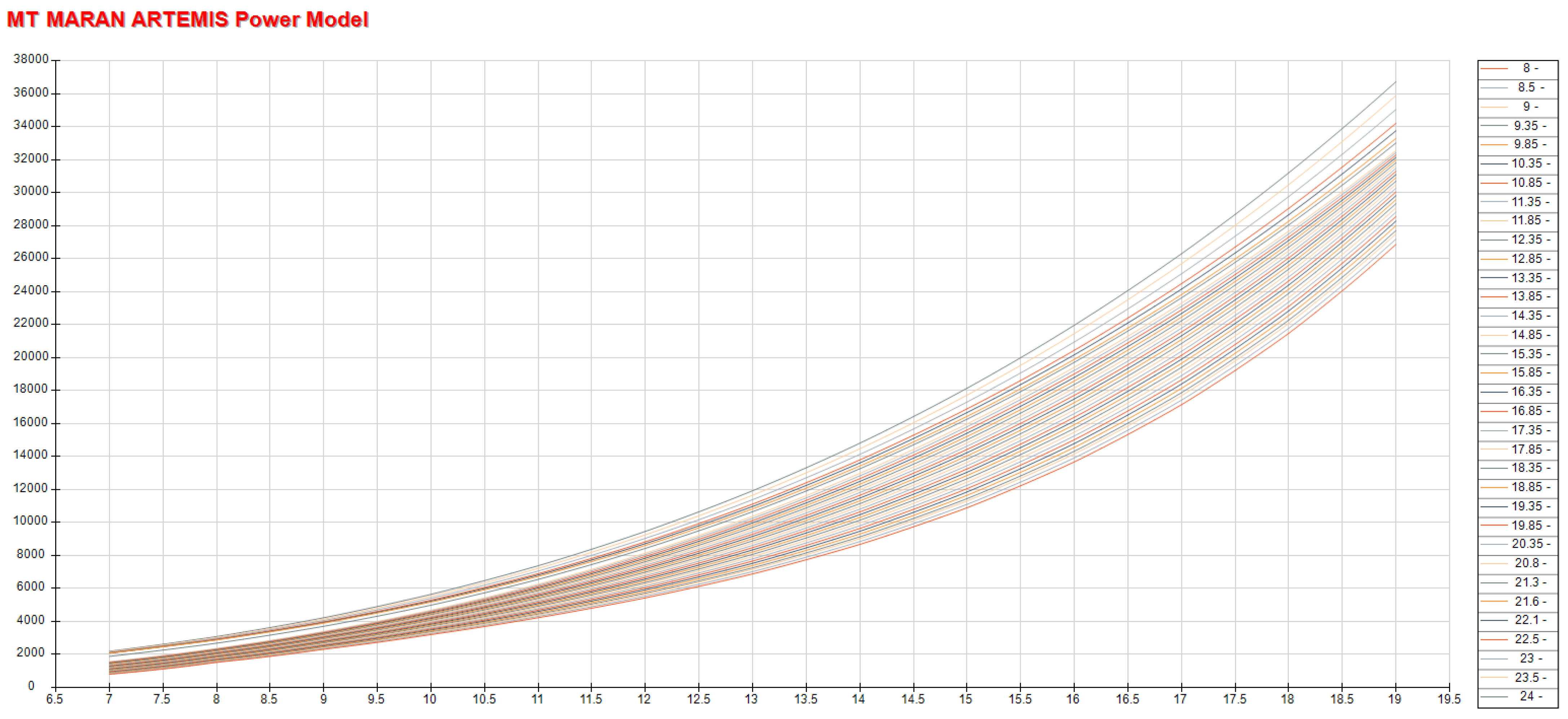
2.2. Baseline Ship Performance Model

Before presenting the mathematical formulation and our methodological workflow, it is crucial to introduce the method that will serve as the baseline for our models. The most common and well-established approach for ship performance modelling used in the shipping industry is the combination of sea trial curves with theoretical formulas, such as Kreitner’s method [41] or ISO-15016 [42]. This approach overcomes the limitations of using sea trial curves regarding changing factors, such as weather conditions, as it accounts for the added resistance due to wind, waves, and currents. It also significantly improves accuracy compared to uncorrected sea trial curves. Moreover, such a method has limited complexity and low computational cost, a crucial criterion for the industry, as it enables its use on vessels with limited resources as the ship performance model for operational optimisations.
At the Angelicoussis Group, a variation of this approach is used as the ship performance model. The sea trial curves for the group of sister vessels under examination are processed and refined following internal experimentation conducted by the Energy Efficient Department delivering the Power Model illustrated in Figure 1, which estimates the expected generated Shaft Power from the ship’s engine with respect to draft and vessel speed under ideal scenarios, such as a clean hull and calm water.
To accommodate for the fouling (i.e., the accumulation and growth of marine plants on the submerged structures of the ship, including the ship’s hull, piers, piling, oil rings, and the internal parts of the pipework used to carry water as a coolant for the shipboard propulsion and power plant, which affects the ship’s performance, as it increases the resistance and thereby the engine requires more fuel to overcome these gradual builds on growth-induced resistance), an empirical roughness factor, designed by the Energy Efficient Department of the Angelicoussis Group based on internal experimentations, is used. It is estimated as follows:
RoughnessFactor = 1 + max ( Days from Delivery , Days from Dry Dock ) 365 2 100
where Days from Delivery and Days from Dry Dock are defined as above.
Finally, regarding the effects of weather on shaft power, the maritime company is using Kreitner’s method, which employs different models to account for the effects of wind, waves, and currents. By amalgamating wind power, wave power, current power, roughness factor, and multiplying the result by the logarithm of the power model, the performance model was evaluated. This model is used currently in the industry for the same operational and environmental conditions, which will serve as a baseline model for our trained models. While this approach provides an accepted reference, it is inherently limited to short-term, steady-state trials. The accuracy of the method also depends heavily on the availability and quality of trial data and experimentation. Furthermore, Kreitner’s weather models’ prediction accuracy drops dramatically when the weather conditions are above 4 degrees on the Beaufort scale. These limitations underscore the need for more adaptive models, such as those proposed in this study, which leverage broader operational datasets and environmental variability to more accurately represent real-world vessel performance across diverse conditions.

2.3. Mathematical Formulation

In mathematical terms, our problem is to find the function f : X R , where X is the space of the operational and environmental conditions and f ( X ) are the possible values of the Shaft Power under those conditions. This is not feasible; therefore, machine learning methods were used to generate the optimal estimate of the function f, by utilising a training set of data { ( x 1 , y 1 ) , , ( x n , y n ) } ( R 12 × R ) n of size n, where x i R 12 is a vector with our observed 12 features that capture the operational and environmental conditions at a specific moment during a voyage, and y i R is the real value of the Shaft Power as generated and measured by the vessels’ engines that the authors would like to predict.
As previously mentioned, the objective is to identify the function f ( X ) = Y ^ for predicting Y ^ , given values of the input X , with the selection criterion for f being defined as follows:
arg min f F L ( Y , f ( X ) )
where L ( Y , f ( X X ) ) is a loss function for penalising errors in prediction. As the loss function, the R 2 metric was used, or the coefficient of determination, which indicates the proportion of variation in the dependent variable explained by the independent variables. It is calculated as follows:
R 2 = 1 i = 1 n y i y ^ i 2 i = 1 n y i y ¯ 2
Higher R 2 values, closer to 1, reflect better model accuracy. This metric offers a comprehensive evaluation of model performance, highlighting accuracy, error magnitude, and predictive reliability.

2.4. Statistical Machine Learning Models and SHAP Method

This section presents the different statistical machine learning methods that were explored for ship performance modelling, along with the SHapley Additive exPlanations (SHAP) method, which offers an understanding of how features influence a model’s predictions. The selected machine learning models represent a diverse set of fundamental methodologies. They include instance-based learning (k-NN), kernel models (SVM), decision tree-based methods (Decision Trees, Random Forest, XGBoost, LightGBM), and neural networks (NNs). This diversity allows for a comprehensive evaluation across different algorithmic principles, ensuring that both simple and complex relationships in the data are effectively explored and benchmarked.

2.4.1. The knn

The first model is the k-NN algorithm, one of the most straightforward machine learning techniques. When handling regression tasks, it predicts the value by utilising a weighted mean function f ^ ( x ) = i = 1 k f ( x i ) k , where f ^ ( x i ) represents the estimated value. Alternatively, more sophisticated functions can be utilised, including inverse distance weighting, as depicted in Equation (4).
f ^ ( x ) = i = 1 k w i ( x 1 , , x k ) f ( x i ) i = 1 k w i ( x 1 , , x k ) if ρ ( x , x i ) 0 i k f ( x i ) otherwise
Within the k-NN algorithm, the model has the flexibility to change the distance function. A common approach involves exploring various values for the Minkowski distance (shown in Equation (5)), which allows for adapting the distance metric to better suit the characteristics of the dataset. More mathematically intricate distance functions can also be employed, such as exponentially weighting by distance or utilising a Gaussian function (Gaussian kernel).
ρ ( x , y ) = i = 1 n x i y i 1 p

2.4.2. Support Vector Machines

Support Vector Machines (SVMs) are powerful supervised learning models. SVM constructs a hyperplane or a set of hyperplanes in a high-dimensional or even infinite-dimensional space, depending on the characteristics of the dataset. Let S = { ( x 1 , y 1 ) , , ( x n , y n ) } be a training dataset, where x i R d and y i { 1 , 1 } . The training dataset is called linearly separable if there exists a hyperplane (hyperspace) ( w , b ) such that for x i holds that y = sign w , x i + b ; alternatively, the latter can be written in the form of inequalities as
y i · w , x i + b > 0 for all x i
The hyperplanes (hyperspaces) which have this property are infinite; therefore, to select the optimal solution, it is important to
arg min ( w , b ) w 2 for all x i : y i · w , x i + b 1
There are several formulations for problems similar to the previous one, which incorporate additional constraints such as the regularisation terms. In such cases, Equation (7) is transformed to the following:
min w , b , ξ λ w 2 + 1 m i = 1 m ξ i for all x i : y i · w , x i + b 1 ξ i and ξ i 0
The linearity is not always the situation which is faced, so a more sophisticated method is to embed our dataset into a higher feature space using the kernel functions. The kernel function K ( x , x ) = ψ ( x ) , ψ ( x ) , where the function ψ is some domain space on some Hilbert space. The more common kernels are
  • The Gaussian kernel which is defined as K ( x , x ) = e x x 2 2 σ = e γ x x 2 .
  • The polynomial kernels which are defined as K ( x , x ) = 1 + γ < x , x > k .
  • The sigmoid kernel which is defined as K ( x , x ) = tanh γ < x , x > + r .

2.4.3. Neural Networks

Neural networks (NNs) have become a cornerstone of modern machine learning, capturing widespread interest in recent years. Despite their current prominence, their conceptual foundations were laid decades ago, inspired by biological processes observed in the human brain. The earliest formalisation of a neural model is credited to McCulloch and Pitts [43], who introduced a simplified abstraction of a neuron aimed at mimicking its basic decision-making behaviour.
Their model defines a function f : R d { 0 , 1 } given by
f ( x 1 , , x d ) = I R + i = 1 d w i x i θ ,
where w i and θ are real-valued parameters, d N , and I R + denotes the indicator function, defined as
I R + ( x ) = 0 , if x < 0 , 1 , if x 0 .
In the context of neural networks, this step function is referred to as the activation function, which determines whether the artificial neuron becomes active based on a weighted combination of its inputs. The former guides us to state that NNs can possess the remarkable property of being universal function approximators. This means they are capable of approximating a wide class of functions to the desired degree of accuracy, provided sufficient depth, width, and appropriate parameters. In particular, even relatively simple architectures, such as feedforward networks with a single hidden layer and a non-linear activation function like the sigmoid, can approximate any continuous function on compact subsets of R n . The following formal statement, knowns as the Universal Approximation Statement [44], illustrates this idea for Lipschitz functions: Let f : [ 1 , 1 ] n [ 1 , 1 ] be a ρ -Lipschitz function. Fix some ε > 0 . Then, there exists a neural network
N : [ 1 , 1 ] n [ 1 , 1 ] ,
with the sigmoid activation function, such that for every x [ 1 , 1 ] n ,
| f ( x ) N ( x ) | ε .
This property can be generalised, and it highlights the expressive power of neural networks [44].

2.4.4. Decision Trees (DTs)

Decision Trees represent a non-parametric, supervised learning methodology applicable to both classification and regression tasks. Mathematically, a Decision Tree is a predictor p : X Y , where X denotes the space of the features and Y is the co-domain space in classification settings. The structure of the tree is formed by recursively partitioning the feature space, typically based on individual features of x or a predefined set of splitting criteria. The goal is to construct a model that can accurately predict the value of a target variable by learning interpretable decision rules derived from the training data [44].

2.4.5. Random Forest

A Random Forest is an ensemble learning method that constructs a collection of Decision Trees, each trained on a subset of the data. Specifically, each tree is generated by applying a learning algorithm A to the training set S along with an additional random vector θ , where θ is drawn independently and identically distributed from a specified distribution. The final prediction of the Random Forest classifier is determined by aggregating the outputs of individual trees, typically through a majority voting scheme [44].

2.4.6. XGBoost and LightGBM

XGBoost falls into the category of tree boosting, a highly effective and widely used machine learning method. Specifically, XGBoost is a scalable, end-to-end tree boosting system that has gained significant popularity among data scientists for delivering state-of-the-art results in numerous machine learning challenges [45]. LightGBM, which stands for Light Gradient-Boosting Machine, is a high-performance, open-source framework for gradient boosting that leverages tree-based learning algorithms. Originally developed by Microsoft, LightGBM is widely used for tasks such as ranking, classification, and other machine learning applications. The framework implements various boosting techniques, including Gradient Boosting Tree (GBT), Gradient Boosting Decision Tree (GBDT), Gradient Boosted Regression Tree (GBRT), Gradient Boosting Machine (GBM), and Multiple Additive Regression Tree (MART). Designed for distributed and efficient computation, LightGBM offers several advantages, including faster training speeds, lower memory usage, enhanced accuracy, and support for parallel, distributed, and GPU-accelerated learning. Furthermore, its capability to handle large-scale datasets makes it an excellent choice for modern machine learning challenges.

2.4.7. SHapley Additive exPlanations

SHAP (SHapley Additive exPlanations) is a cutting-edge method for understanding how features influence a model’s predictions. It adheres to key principles of accuracy, completeness, and consistency, ensuring reliable and interpretable explanations for a wide array of models, from simple Linear Regression to complex deep learning models like transformers used in natural language processing. Although alternative explainability methods such as LIME and DeepLIFT exist [46], SHAP was selected due to its strong theoretical foundation and broad applicability. SHAP unifies these approaches through a game-theoretic framework based on Shapley values, offering consistent and locally accurate feature attributions. This makes it particularly well suited for comparing multiple model types in a unified, interpretable manner. SHAP excels in handling the complexities of correlated features, making it a versatile and powerful tool for gaining insights into both simple and complex machine learning models. The SHAP method, which belongs to additive feature attribution methods, has the following properties: (a) Local accuracy: This property indicates that SHAP values offer a precise and localised interpretation of the model’s prediction for a particular input. (b) Missingness: This ensures robustness to missing data and prevents irrelevant features from skewing the interpretation. (c) Consistency: The values remain constant unless there is a change in the contribution of a feature. Consequently, they offer a consistent interpretation of the model’s behaviour, even amidst alterations in the model architecture or parameters.

2.5. The Hyperparameter Combinations

In this study, various machine learning models were employed, each with a range of hyperparameter combinations. For neural networks (NNs), the activation functions used were “tanh” and “relu,” with hidden layer sizes of 5, 10, 20, and 50. The learning rates tested were 0.01, 0.1, and 0.2, and the “adam” solver was utilised. For Random Forests (RFs), the number of estimators was set at 50, 100, and 200, using “absolute error” as the criterion and a maximum depth of 10.
The k-Nearest Neighbours (KNN) model was evaluated with distance metrics corresponding to p values of 1, 1.5, 2, and 3, and the number of neighbours considered was 5, 10, 25, 50, 100, and 150. Both “uniform” and “distance” weight functions were applied. For XGBoost, hyperparameters included lambda values of 1 and 10, with 100, 300, and 500 estimators. The learning rates were set at 0.01 and 0.05, and maximum depths of 5, 10, and 20 were explored.
In the LightGBM framework, the number of leaves was tested at 31, 50, and 100, with estimators ranging from 100 to 500. The learning rates were 0.01, 0.1, and 0.2, and the maximum depths were set at 5, 10, and 20. The Support Vector Machine (SVM) model used a linear kernel, with C values of 0.1 and 1 and epsilon values of 0.01 and 0.1. Lastly, for Decision Trees (DTs), the minimum number of samples required to split an internal node was tested at 2, 5, 10, 20, and 50.
This exploration of hyperparameters allowed for a thorough evaluation of each model’s performance across a wide range of configurations.

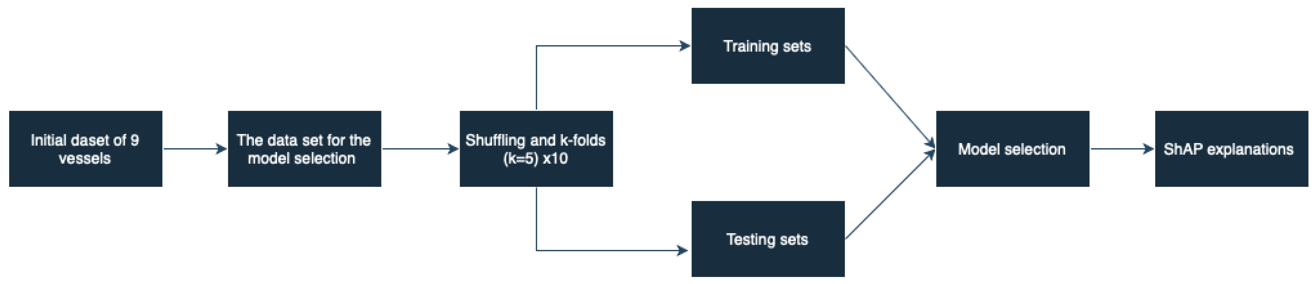
2.6. Methodological Workflow

In this study, a range of machine learning models, described in Section 2.4, were evaluated to identify the most effective model for predicting the shaft power in real-world conditions. To ensure rigorous model development and unbiased performance assessment, following established machine learning best practices for reliable model evaluation, we implement a partitioning strategy that includes all best practices. For the model development, evaluation and selection, i.e., for model training and hyperparameter optimisation (see hyperparameter configurations, in Table 3), we employed a dataset that was collected from nine vessels and comprised approximately 168K samples. The selection of hyperparameter ranges was guided by the number of input features and the specific characteristics of each model. A grid search approach was used to explore combinations, resulting in a broad range of values. Initial values were chosen based on standard practices in the literature and adjusted to reflect each algorithm’s behaviour, such as model depth for neural networks and learning rate sensitivity.
Our model development and selection process employs a two-step validation approach to maximise robustness. First, we repeatedly partition the development data into training (80%) and validation (20%) subsets, performing this step 10 times through repeated shuffling to ensure robust model training. Second, a five-fold cross-validation technique is applied within each training set to further refine the model parameters and mitigate overfitting. This comprehensive validation strategy during the development phase allows us to identify optimal model configurations while maintaining the integrity of our final evaluation.
This methodological and rigorous workflow, depicted in Figure 2, ensures that our performance metrics reflect true generalisation ability and are reliable and unbiased.

3. Results

3.1. Model Selection Results
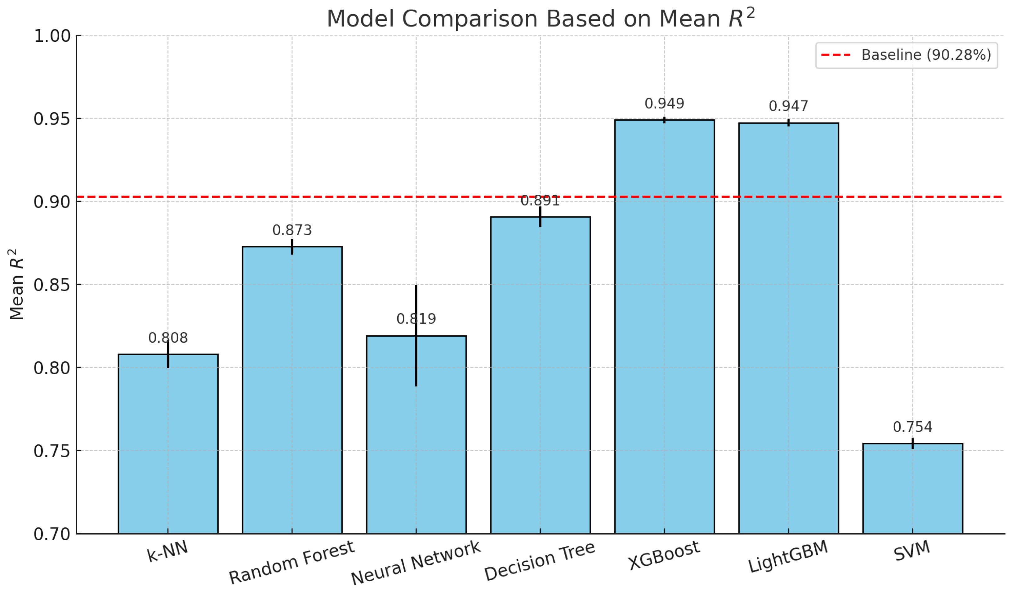
This section presents a detailed analysis of the performance of various machine learning models during the model development phase. The models are evaluated using the R 2 metric, which measures the proportion of variance explained by the model. Performance stability is further characterised by standard deviations (SDs) and 95% confidence intervals (CIs) across repeated runs. Table 4 presents the model selection results based on the validation dataset.
In more details, the best K-Nearest Neighbours model (five neighbours, p = 1.0 for Manhattan distance, distance weighting) achieved a mean RMSE of 1723.41291 and a mean R 2 of 0.8081, indicating that the model explains about 80.8% of the variance in the target variable, while the standard deviation of 0.0041 across multiple runs reflects consistent performance. Additionally, the confidence interval (95%) ranged from 0.8074 to 0.8089, further validating the model’s stability and reliability. Overall, this result demonstrates moderate predictive accuracy for this model.
Regarding the Random Forest models, they were evaluated using two criteria: friedman_mse and squared_error. Both configurations used 200 estimators and achieved a mean RMSE of 1405.59474 and nearly identical mean R 2 values of approximately 0.8728. This indicates that Random Forest models captured 87.3% of the variance, showcasing strong predictive capabilities. The standard deviation of these models was exceptionally low at around 0.0024, highlighting their stability. Confidence intervals for both configurations were narrow, with lower and upper bounds closely centred around the mean, demonstrating highly reliable performance across evaluations.
Neural networks were tested with different hidden layer configurations. A model with 50 hidden layers, combined with the adam optimiser, a learning rate of 0.01 and ReLU activation function, achieved a mean RMSE of 1671.11765 and the highest mean R 2 of 0.8193. This configuration outperformed the smaller network with 20 hidden layers with the same hyperparameters, which yielded a mean R 2 of 0.8143. Despite their accuracy, Neural Networks showed slightly higher variability, with standard deviations of 0.0153 and 0.0161 for the 50- and 20-layer configurations, respectively. Confidence intervals were wider than those observed for ensemble methods, indicating that while neural networks perform well, they exhibit less stability compared to models like Random Forest and XGBoost.
Despite its simplicity, the best Decision Tree model, using a minimum sample split of 20 and a mean RMSE of 1299.57351 , achieved a mean R 2 of 0.8909. This result is among the highest single-model performances, demonstrating its capability to explain 89.1% of the variance in the target variable. The standard deviation was low (0.0031), indicating consistent results across runs, while the narrow confidence interval, ranging from 0.8905 to 0.8912, further confirms the reliability of the Decision Tree model.
XGBoost emerged as the best-performing model, achieving a maximum mean R 2 of 0.9490 with λ = 10 , 500 estimators, a learning rate of 0.05, and a maximum depth of 20. Reducing the number of estimators to 300 slightly lowered the mean RMSE to 888.29617 and the mean R 2 to 0.9482, indicating diminishing returns with fewer trees. The standard deviation for XGBoost was extremely low (0.00093), reflecting high stability in predictions. Confidence intervals were exceptionally narrow, such as [0.9488, 0.9492], making XGBoost the most consistent and accurate model for these dataset.
LightGBM also demonstrated excellent performance, with the best configuration achieving a mean R 2 of 0.9474. This configuration used 100 leaves, 500 estimators, a learning rate of 0.2, and a maximum depth of 20. Other configurations, such as reducing the depth to 10 or lowering the learning rate to 0.1, resulted in slightly lower RMSE values of 902.16747 and R 2 values of 0.9425. The standard deviation for LightGBM was slightly higher than XGBoost but still low (0.0011 to 0.0012). Confidence intervals remained narrow across all configurations, confirming stable performance. LightGBM provides an excellent balance between accuracy and computational efficiency.
The best Support Vector Machine model (linear kernel, regularisation parameter C = 1.0 , ϵ = 0.01 ) achieved a mean RMSE of 1949.72586 and a mean R 2 of 0.7544. While this performance is lower compared to ensemble methods, it demonstrates moderate predictive accuracy. The standard deviation was low (0.0017) and the confidence interval was narrow ([0.7541, 0.7547]), indicating stable but less competitive performance compared to other models.
Among all models (see Table 5 and Figure 3), XGBoost emerged as the top performer, achieving the highest mean R 2 score of 0.9490, indicating excellent predictive power and minimal variance across runs and demonstrating excellent stability with minimal variance. LightGBM followed closely with a mean R 2 of 0.9474, demonstrating robust performance, making it another highly reliable choice. Decision Trees and Random Forests achieved strong scores as well (0.8909 and 0.8728, respectively), showcasing their effectiveness despite their lower complexity. Neural networks showed good performance with mean R 2 values exceeding 0.81; however, they exhibited higher variance, indicating less stability compared to ensemble methods. Finally, K-NN and SVM models exhibited moderate predictive capabilities, with mean R 2 values of 0.8081 and 0.7544, respectively. Overall, ensemble methods such as XGBoost and LightGBM demonstrated the best trade-off between accuracy, stability, and reliability, and emerged as the most reliable and accurate for shaft power estimation.
Each bar in Figure 4 represents the mean R 2 value achieved by a different machine learning model, providing a visual comparison of their predictive performance. The red dashed line indicates that the mean baseline value of R 2 is 90.2 and it is almost equal to 1500 for the RMSE, serving as a reference point to easily identify models that perform above or below this threshold. Additionally, the exact R 2 values are labelled above each bar to facilitate a quick and precise comparison between models.
The baseline mean R 2 value is 0.9028. Based on the model performances, we recorded the following:
  • k-NN achieved a mean R 2 of 0.8081, which is lower than the baseline.
  • Random Forest achieved a mean R 2 of 0.8728, which is lower than the baseline.
  • Neural networks achieved a mean R 2 of 0.8193, which is lower than the baseline.
  • Decision Tree achieved a mean R 2 of 0.8909, which is slightly lower than the baseline.
  • XGBoost achieved a mean R 2 of 0.9490, which is higher than the baseline, indicating better performance.
  • LightGBM achieved a mean R 2 of 0.9474, which is also higher than the baseline, indicating better performance.
  • SVM achieved a mean R 2 of 0.7544, which is lower than the baseline.
When evaluating models based on the Root Mean Squared Error (RMSE), the following insights emerged:
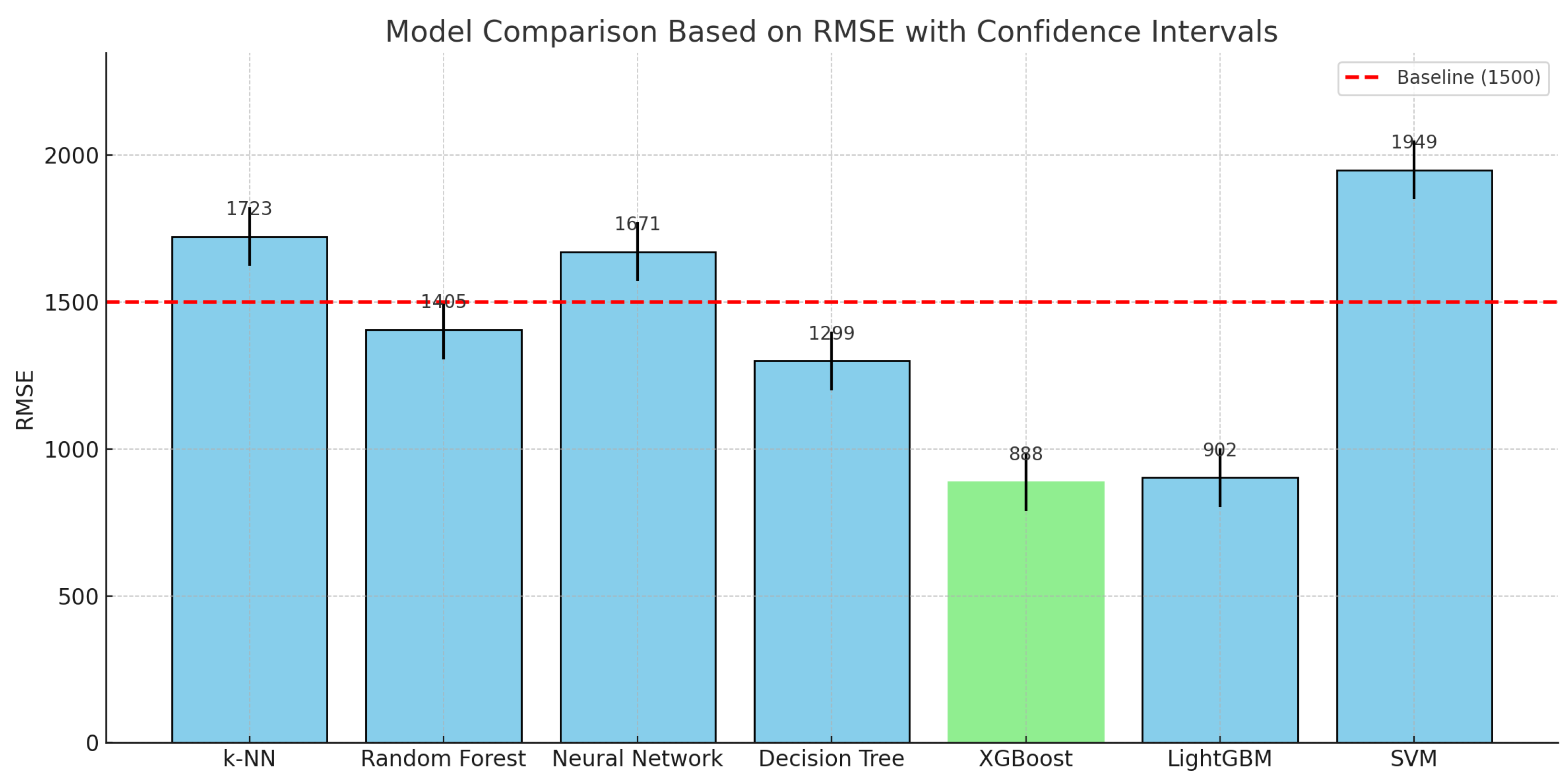
  • XGBoost achieved the lowest RMSE of 888.30, indicating the highest accuracy in absolute prediction error.
  • LightGBM closely followed with an RMSE of 902.17, also showing excellent performance.
  • Decision Tree achieved an RMSE of 1299.57, outperforming more complex models like k-NN and neural networks.
  • Random Forest achieved a high RMSE of 1405.59.
  • Neural networks and k-NN showed higher RMSE values of 1671.12 and 1723.41, respectively.
  • SVM had the highest RMSE of 1949.73, indicating the weakest performance in this context.
In conclusion, only XGBoost and LightGBM outperformed the baseline, with XGBoost showing the highest mean R 2 of 0.9490, followed closely by LightGBM with a mean R 2 of 0.9474. All other models exhibited lower predictive performance compared to the baseline.
Computational efficiency constitutes a critical aspect in the practical deployment of machine learning algorithms, particularly in environments with constrained processing resources such as onboard ship systems. To account for this, we incorporated a systematic assessment of execution times, separately evaluating training and inference durations (Table 6). All models were evaluated under a CPU-only setting to ensure consistency and eliminate variability due to hardware acceleration. This analysis is intended to complement the accuracy-based evaluation by providing performance indicators that are directly relevant to real-world deployment scenarios.

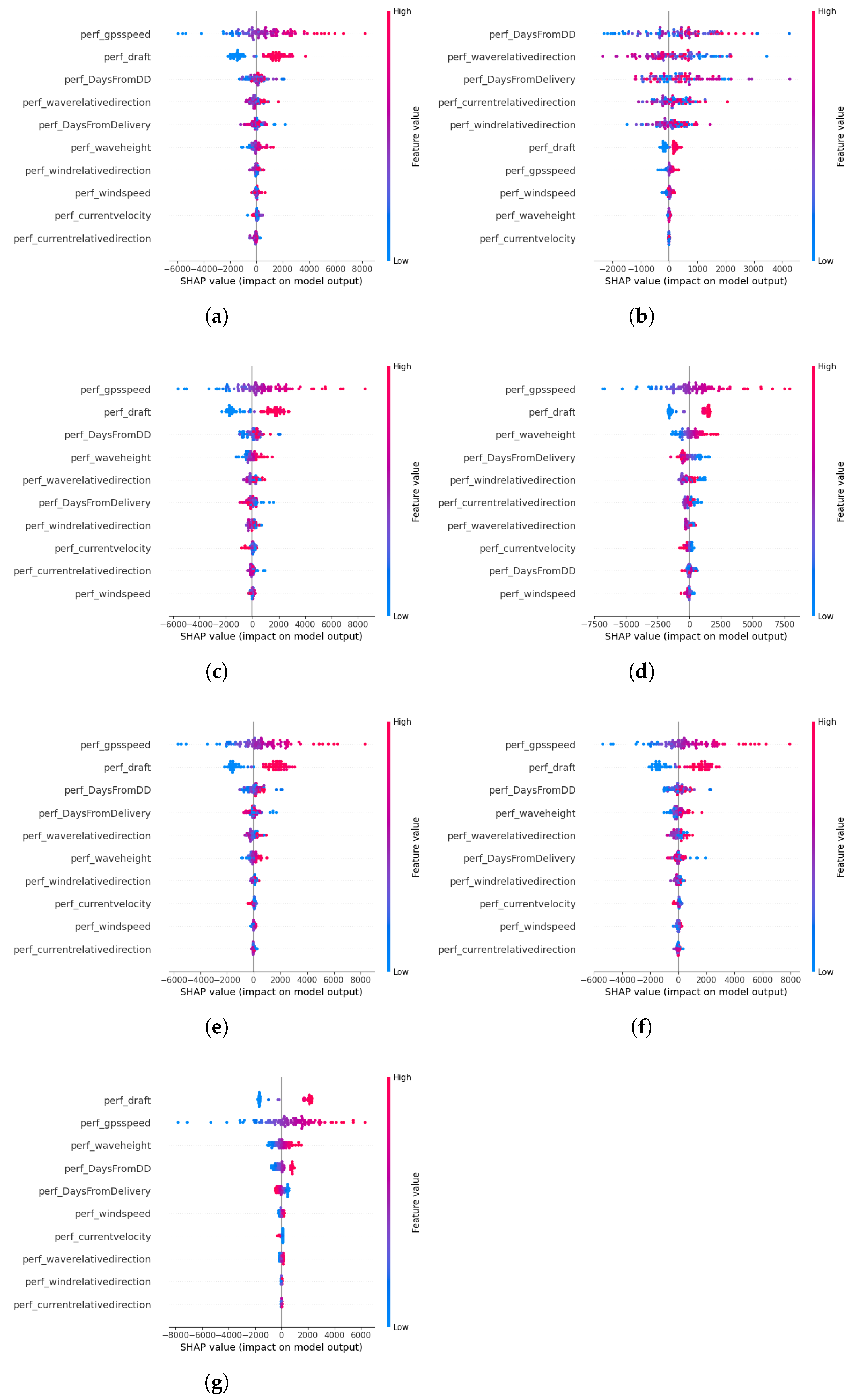
3.2. SHAP Explanations

This section presents and interprets SHAP summary graphs for each machine learning model employed in this study. The plots in Figure 5 visualise the magnitude and direction of the contribution of features to individual predictions, i.e., how individual features affect predictions, offering insights into the behaviour and interpretability of the model. Specifically, positive SHAP values indicate features that increase the predicted outcome, while negative values represent decreasing effects. The horizontal spread of SHAP values illustrates how the impact of the feature varies between instances, and the associated colour gradient, from red (high feature values) to blue (low feature values), helps to interpret the influence of individual observations.
The SHAP summary plot for the Decision Tree model highlights that Days from Dry Dock and Draft exhibit the highest SHAP values, signifying their dominant role in shaping the model’s output. The k-Nearest Neighbors model reveals that Days from Dry Dock and Days from Delivery are the most influential variables. Although k-NN is a non-parametric model, the SHAP values offer a valuable explanation of how feature values shape predictions. The plot shows that the impact of each feature varies considerably between samples, revealing localised importance and helping to address the interpretability challenges commonly associated with distance-based models.
For the LightGBM model, SHAP analysis once again highlights Days from Dry Dock and Draft as the most critical features. Sharp concentrations of SHAP values in certain areas of the plot suggest that the model has learned specific feature interactions or rule-like behaviours. Compared to simpler models, LightGBM displays a wider range of SHAP distributions, reflecting the nuanced and data-driven decision boundaries learned during training.
In the case of the neural network model, SHAP values emphasise the significant contributions of GPS speed and Wave Height. The wide dispersion of SHAP values across samples underscores the model’s ability to capture complex, non-linear interactions. In addition, the colour gradients within the graph reveal how high the feature values (such as for Days from Dry Dock) consistently influence the model in a particular direction, further illuminating the behaviour of the model.
The Random Forest model exhibits SHAP patterns characteristic of tree-based ensembles. Notably, Draft and Days from Dry Dock emerge as key predictors. The clustered appearance of SHAP values is likely due to the model’s discrete decision thresholds. This structure results in a broad distribution of feature contributions across the dataset, revealing considerable variability in how the model assigns importance to different features depending on the input.
XGBoost, as a gradient-boosted ensemble, shows a refined and compact spread of SHAP values. The model heavily relies on Days from Dry Dock and Wave Height, both of which display broad and well-defined SHAP distributions. High values of these features (indicated in red) frequently correspond to positive SHAP contributions, suggesting their consistent influence in driving the prediction upward. The sharply defined value regions in the SHAP plot reflect the model’s finely tuned learning process.
For the SVM model, the SHAP plot reveals a narrower range of feature impacts compared to tree-based models. While Draft and GPS Speed contribute moderately to the predictions, the overall effect of features is more evenly distributed. The model does not produce high-magnitude SHAP values, which aligns with its smoother decision boundaries and lack of inherent probabilistic output. Nonetheless, SHAP analysis reveals the model’s sensitivity to specific feature values, captured through mild clustering in the plot.
Overall, a comparison across models shows that Days from Dry Dock, Draft, and GPS Speed consistently rank among the most influential features. Tree-based models—such as the Decision Tree, Random Forest, LightGBM, and XGBoost—display more concentrated and interpretable SHAP patterns, making them particularly suitable for explainable decision-making contexts. Conversely, models like k-NN, SVM, and neural networks exhibit a more distributed feature influence, often requiring SHAP to reveal latent relationships. Ultimately, the use of SHAP improves transparency across all model types and provides valuable insights into feature relevance and prediction dynamics.

4. Conclusions

This study demonstrates the efficacy of integrating machine learning and explainable AI techniques in the domain of shaft power estimation for large marine vessels. Using a comprehensive dataset from VLCCs spanning three years of operation, we developed predictive models capable of accurately estimating shaft power under varying operational and environmental conditions. Among the models evaluated, XGBoost emerged as the best-performing algorithm, achieving R 2 = 0.9490 on the validation set, followed by LightGBM with R 2 = 0.9474 . Both ensemble methods outperformed the traditional industry baseline model ( R 2 = 0.9028 ), corresponding to relative improvements of approximately 5.1% and 4.8%, respectively.
To enhance transparency, we incorporated SHAP (SHapley Additive exPlanations) into our modelling pipeline. This approach allowed us to quantify and visualise the contribution of each input variable to the final prediction, addressing one of the major criticisms of black-box machine learning models—lack of interpretability. Variables such as draft, GPS speed, and maintenance-related metrics (e.g., time since dry dock) consistently ranked among the most influential features, offering domain-relevant insights that align with physical expectations and marine engineering principles.
Compared to traditional estimation techniques—often based on sea trial curves and empirically derived correction factors—the proposed data-driven approach offers superior adaptability, accuracy, and generalisation. Traditional models tend to be rigid and assume constant operating conditions, whereas our models account for the full spectrum of real-world variation, including weather effects, operational profiles, and degradation over time.
The inclusion of the RMSE in our evaluation provides a practical measure of the model’s prediction error in physical units. For example, the XGBoost model achieved an RMSE of 888.30∼kW, which—given typical fuel consumption rates of 150–300∼g/kWh—translates to an uncertainty of roughly 130–210∼kg of fuel per hour. This level of accuracy supports use in operational settings, where reliable shaft power estimates are essential for fuel efficiency monitoring, emission tracking, and voyage optimisation. Moreover, the high R 2 values across models confirm the soundness and completeness of the dataset, indicating that the model effectively captures the core dynamics of marine propulsion.
Furthermore, our findings suggest that machine learning can serve not only as a performance estimation tool but also as a decision support system for operational optimisation, fleet management, and regulatory compliance. By integrating explainability into the modelling framework, we build user trust and open avenues for practical deployment on board ships and within shore-based monitoring systems.
The proposed models can support voyage optimisation by predicting shaft power under varying weather and loading conditions, allowing route planners to minimise fuel consumption. Additionally, the insights provided by SHAP can inform maintenance decisions, such as scheduling hull cleaning based on performance degradation patterns. Future work could extend this framework to include emission prediction, optimisation of voyage planning, and real-time integration with weather forecasts. Another promising direction lies in the application of federated learning across fleets, enabling data privacy while using distributed intelligence. As the maritime industry continues its digital transformation, explainable machine learning offers a powerful tool for achieving environmental, economic, and operational goals.

Author Contributions

Conceptualisation, Y.K., T.P. and I.F.; methodology, S.Z., K.G., D.K. and Y.K.; software, S.Z., K.G. and D.K.; validation, S.Z., K.G., Z.L., D.P., I.F. and Y.K.; formal analysis, Y.K.; investigation, Z.L., D.P., I.F. and Y.K.; resources, Z.L., D.P. and I.F.; data curation, S.Z., K.G., Z.L., D.P., I.F. and Y.K.; writing—original draft preparation, S.Z. and K.G.; writing—review and editing, S.Z., K.G., I.F. and Y.K.; visualisation, S.Z.; supervision, T.P., I.F. and Y.K.; project administration, Y.K. All authors have read and agreed to the published version of the manuscript.

Funding

This research received no external funding.

Data Availability Statement

The data presented in this study are available on request from the corresponding author.

Conflicts of Interest

Authors Zoran Lajic and Dimitris Papathanasiou were employed by the company Angelicoussis group. The remaining authors declare that the research was conducted in the absence of any commercial or financial relationships that could be construed as a potential conflict of interest.

Abbreviations

The following abbreviations are used in this manuscript:
ANNArtificial Neural Network
CNNConvolutional Neural Network
DTDecision Tree
ENNEnsemble Neural Network
ETExtra Tree
GPRGaussian Process Regression
GTBMGradient Tree Boosting Machine
IoTInternet of Things
knnK Nearest Neighbours
LGBMLight Gradient Boosting Machine
LRLinear Regression
MLPMulti-layer Perceptron
MLRMultiple Linear Regression
NL-PCRnon-linear Principal Component Regression
NL-PLSRnon-linear Partial Least Squares Regression
NOAANational Oceanic and Atmospheric Administration
RFRandom Forest
RNNRecurrent Neural Network
RRRidge Regression
RTRegression Tree
SGDsSustainable Development Goals
SHAPSHapley Additive exPlanations
SVMSupport Vector Machine
SVRSupport Vector Regression
VLCCsVery Large Crude Carriers

References

  1. Lee, B.X.; Kjaerulf, F.; Turner, S.; Cohen, L.; Donnelly, P.D.; Muggah, R.; Davis, R.; Realini, A.; Kieselbach, B.; MacGregor, L.S.; et al. Transforming Our World: Implementing the 2030 Agenda Through Sustainable Development Goal Indicators. J. Public Health Policy 2016, 37, 13–31. [Google Scholar] [CrossRef]
  2. Wang, X.; Yuen, K.F.; Wong, Y.D.; Li, K.X. How can the maritime industry meet Sustainable Development Goals? An analysis of sustainability reports from the social entrepreneurship perspective. Transp. Res. Part D Transp. Environ. 2020, 78, 102173. [Google Scholar] [CrossRef]
  3. Farkas, A.; Degiuli, N.; Martić, I.; Vujanović, M. Greenhouse gas emissions reduction potential by using antifouling coatings in a maritime transport industry. J. Clean. Prod. 2021, 295, 126428. [Google Scholar] [CrossRef]
  4. Huang, J.; Duan, X. A comprehensive review of emission reduction technologies for marine transportation. J. Renew. Sustain. Energy 2023, 15, 032702. [Google Scholar] [CrossRef]
  5. Morobé, C. 3 Examples of How Improved Ship Performance Modelling Can Save Fuel. White Paper, Torqua AI, 2022. Available online: https://toqua.ai/whitepapers/3-examples-of-how-improved-ship-performance-modelling-can-save-fuel (accessed on 1 June 2025).
  6. Gupta, P.; Rasheed, A.; Steen, S. Ship performance monitoring using machine-learning. Ocean Eng. 2022, 254, 111094. [Google Scholar] [CrossRef]
  7. Lang, X.; Wu, D.; Mao, W. Comparison of supervised machine learning methods to predict ship propulsion power at sea. Ocean Eng. 2022, 245, 110387. [Google Scholar] [CrossRef]
  8. Laurie, A.; Anderlini, E.; Dietz, J.; Thomas, G. Machine learning for shaft power prediction and analysis of fouling related performance deterioration. Ocean Eng. 2021, 234, 108886. [Google Scholar] [CrossRef]
  9. Kim, D.; Lee, S.; Lee, J. Data-Driven Prediction of Vessel Propulsion Power Using Support Vector Regression with Onboard Measurement and Ocean Data. Sensors 2020, 20, 1588. [Google Scholar] [CrossRef]
  10. Kriezis, A.C.; Sapsis, T.; Chryssostomidis, C. Predicting Ship Power Using Machine Learning Methods. In Proceedings of the SNAME Maritime Convention, Houston, TX, USA, 29 September 2022; p. D031S017R005. [Google Scholar] [CrossRef]
  11. Kim, H.S.; Roh, M.I. Interpretable, data-driven models for predicting shaft power, fuel consumption, and speed considering the effects of hull fouling and weather conditions. Int. J. Nav. Archit. Ocean Eng. 2024, 16, 100592. [Google Scholar] [CrossRef]
  12. Radonjic, A.; Vukadinovic, K. Application of ensemble neural networks to prediction of towboat shaft power. J. Mar. Sci. Technol. 2015, 20, 64–80. [Google Scholar] [CrossRef]
  13. Parkes, A.; Sobey, A.; Hudson, D. Physics-based shaft power prediction for large merchant ships using neural networks. Ocean Eng. 2018, 166, 92–104. [Google Scholar] [CrossRef]
  14. Sun, L.; Liu, T.; Xie, Y.; Zhang, D.; Xia, X. Real-time power prediction approach for turbine using deep learning techniques. Energy 2021, 233, 121130. [Google Scholar] [CrossRef]
  15. Kim, D.; Handayani, M.P.; Lee, S.; Lee, J. Feature Attribution Analysis to Quantify the Impact of Oceanographic and Maneuverability Factors on Vessel Shaft Power Using Explainable Tree-Based Model. Sensors 2023, 23, 1072. [Google Scholar] [CrossRef]
  16. Kim, Y.C.; Kim, K.S.; Yeon, S.; Lee, Y.Y.; Kim, G.D.; Kim, M. Power Prediction Method for Ships Using Data Regression Models. J. Mar. Sci. Eng. 2023, 11, 1961. [Google Scholar] [CrossRef]
  17. Coraddu, A.; Oneto, L.; Baldi, F.; Anguita, D. Vessels fuel consumption forecast and trim optimisation: A data analytics perspective. Ocean Eng. 2017, 130, 351–370. [Google Scholar] [CrossRef]
  18. Tarelko, W.; Rudzki, K. Applying artificial neural networks for modelling ship speed and fuel consumption. Neural Comput. Appl. 2020, 32, 17379–17395. [Google Scholar] [CrossRef]
  19. Wang, S.; Ji, B.; Zhao, J.; Liu, W.; Xu, T. Predicting ship fuel consumption based on LASSO regression. Transp. Res. Part D Transp. Environ. 2018, 65, 817–824. [Google Scholar] [CrossRef]
  20. Hajli, K.; Rönnqvist, M.; Dadouchi, C.; Audy, J.F.; Cordeau, J.F.; Warya, G.; Ngo, T. A fuel consumption prediction model for ships based on historical voyages and meteorological data. J. Mar. Eng. Technol. 2024, 23, 439–450. [Google Scholar] [CrossRef]
  21. Le, T.T.; Sharma, P.; Pham, N.D.K.; Le, D.T.N.; Van Vang Le, S.M.O.; Rowinski, L.; Tran, V.D. Development of comprehensive models for precise prognostics of ship fuel consumption. J. Mar. Eng. Technol. 2024, 23, 451–465. [Google Scholar] [CrossRef]
  22. Uyanık, T.; Karatuğ, Ç.; Arslanoğlu, Y. Machine learning approach to ship fuel consumption: A case of container vessel. Transp. Res. Part D Transp. Environ. 2020, 84, 102389. [Google Scholar] [CrossRef]
  23. Hu, Z.; Jin, Y.; Hu, Q.; Sen, S.; Zhou, T.; Osman, M.T. Prediction of fuel consumption for enroute ship based on machine learning. IEEE Access 2019, 7, 119497–119505. [Google Scholar] [CrossRef]
  24. Kim, Y.R.; Jung, M.; Park, J.B. Development of a fuel consumption prediction model based on machine learning using ship in-service data. J. Mar. Sci. Eng. 2021, 9, 137. [Google Scholar] [CrossRef]
  25. Moreira, L.; Vettor, R.; Guedes Soares, C. Neural network approach for predicting ship speed and fuel consumption. J. Mar. Sci. Eng. 2021, 9, 119. [Google Scholar] [CrossRef]
  26. Gkerekos, C.; Lazakis, I.; Theotokatos, G. Machine learning models for predicting ship main engine Fuel Oil Consumption: A comparative study. Ocean Eng. 2019, 188, 106282. [Google Scholar] [CrossRef]
  27. Fahrnholz, S.F.; Caprace, J.D. A machine learning approach to improve sailboat resistance prediction. Ocean Eng. 2022, 257, 111642. [Google Scholar] [CrossRef]
  28. Sun, Q.; Zhang, M.; Zhou, L.; Garme, K.; Burman, M. A machine learning-based method for prediction of ship performance in ice: Part I. ice resistance. Mar. Struct. 2022, 83, 103181. [Google Scholar] [CrossRef]
  29. Bassam, A.M.; Phillips, A.B.; Turnock, S.R.; Wilson, P.A. Ship speed prediction based on machine learning for efficient shipping operation. Ocean Eng. 2022, 245, 110449. [Google Scholar] [CrossRef]
  30. Coraddu, A.; Oneto, L.; Baldi, F.; Cipollini, F.; Atlar, M.; Savio, S. Data-driven ship digital twin for estimating the speed loss caused by the marine fouling. Ocean Eng. 2019, 186, 106063. [Google Scholar] [CrossRef]
  31. Chen, Z.S.; Lam, J.S.L.; Xiao, Z. Prediction of harbour vessel emissions based on machine learning approach. Transp. Res. Part D Transp. Environ. 2024, 131, 104214. [Google Scholar] [CrossRef]
  32. Sang, H.; You, Y.; Sun, X.; Zhou, Y.; Liu, F. The hybrid path planning algorithm based on improved A* and artificial potential field for unmanned surface vehicle formations. Ocean Eng. 2021, 223, 108709. [Google Scholar] [CrossRef]
  33. Zissis, D.; Xidias, E.K.; Lekkas, D. A cloud based architecture capable of perceiving and predicting multiple vessel behaviour. Appl. Soft Comput. 2015, 35, 652–661. [Google Scholar] [CrossRef]
  34. Aizpurua, J.I.; Knutsen, K.E.; Heimdal, M.; Vanem, E. Integrated machine learning and probabilistic degradation approach for vessel electric motor prognostics. Ocean Eng. 2023, 275, 114153. [Google Scholar] [CrossRef]
  35. Soner, O.; Akyuz, E.; Celik, M. Statistical modelling of ship operational performance monitoring problem. J. Mar. Sci. Technol. 2019, 24, 543–552. [Google Scholar] [CrossRef]
  36. Lee, Y.E.; Kim, B.K.; Bae, J.H.; Kim, K.C. Misalignment detection of a rotating machine shaft using a support vector machine learning algorithm. Int. J. Precis. Eng. Manuf. 2021, 22, 409–416. [Google Scholar] [CrossRef]
  37. Panagiotakopoulos, T.; Filippopoulos, I.; Filippopoulos, C.; Filippopoulos, E.; Lajic, Z.; Violaris, A.; Chytas, S.P.; Kiouvrekis, Y. Vessel’s trim optimization using IoT data and machine learning models. In Proceedings of the 2022 13th International Conference on Information, Intelligence, Systems and Applications (IISA), Rhodes, Greece, 18–20 July 2022; pp. 1–5. [Google Scholar] [CrossRef]
  38. Filippopoulos, I.; Stamoulis, G. Collecting and using vessel’s live data from on board equipment using “Internet of Vessels (IoV) platform” (May 2017). In Proceedings of the 2017 South Eastern European Design Automation, Computer Engineering, Computer Networks and Social Media Conference (SEEDA-CECNSM), Rhodes, Greece, 24–26 July 2017; pp. 1–6. [Google Scholar] [CrossRef]
  39. Filippopoulos, I.; Stamoulis, G.; Sovolakis, I. Transferring Structured Data and applying business processes in remote Vessel’s environments using the “InfoNet” Platform. In Proceedings of the 2018 South-Eastern European Design Automation, Computer Engineering, Computer Networks and Society Media Conference (SEEDA-CECNSM), Rhodes, Greece, 24–26 July 2018; pp. 1–6. [Google Scholar] [CrossRef]
  40. Filippopoulos, I.; Panagiotakopoulos, T.; Skiadas, C.; Triantafyllou, S.M.; Violaris, A.; Kiouvrekis, Y. Live Vessels’ Monitoring using Geographic Information and Internet of Things. In Proceedings of the 13th International Conference on Information, Intelligence, Systems and Applications, IISA 2022, Corfy, Greece, 18–20 July 2022. [Google Scholar]
  41. Kreitner, J. Heave, pitch, and resistance of ships in a seaway. Trans. R. Inst. Nav. Archit. 1939, 87. [Google Scholar]
  42. ISO 15016:2015; Ships and Marine Technology—Guidelines for the Assessment of Speed and Power Performance by Analysis of Speed Trial Data. The International Organization for Standardization: Geneva, Switzerland, 2015. Available online: https://www.iso.org/standard/61902.html (accessed on 1 June 2025).
  43. McCulloch, W.S.; Pitts, W. A logical calculus of the ideas immanent in nervous activity. Bull. Math. Biophys. 1943, 5, 115–133. [Google Scholar] [CrossRef]
  44. Shalev-Shwartz, S.; Ben-David, S. Understanding Machine Learning: From Theory to Algorithms; Cambridge University Press: New York, NY, USA, 2014. [Google Scholar]
  45. Chen, T.; Guestrin, C. XGBoost: A Scalable Tree Boosting System. In Proceedings of the 22nd ACM SIGKDD International Conference on Knowledge Discovery and Data Mining, KDD ’16, New York, NY, USA, 13–17 August 2016; pp. 785–794. [Google Scholar] [CrossRef]
  46. Ribeiro, M.T.; Singh, S.; Guestrin, C. “Why Should I Trust You?”: Explaining the Predictions of Any Classifier. In Proceedings of the 22nd ACM SIGKDD International Conference on Knowledge Discovery and Data Mining, KDD ’16, New York, NY, USA, 13–17 August 2016; pp. 1135–1144. [Google Scholar] [CrossRef]
Figure 1. Power model for the group of sister vessels examined in this paper. On the X-axis is the vessel speed in knots, on Y-axis is shaft power in Kilo-Watts, and the legend is the draft in meters.
Futureinternet 17 00264 g001
Figure 2. The methodological workflow.
Futureinternet 17 00264 g002
Figure 3. Model comparison based on mean RMSE values with 95% confidence intervals shown as error bars.
Futureinternet 17 00264 g003
Figure 4. Model comparison based on mean R 2 values with 95% confidence intervals shown as error bars. The red dashed line represents the baseline model performance (90.28%).
Futureinternet 17 00264 g004
Figure 5. SHAP summary plots showing feature importance across different machine learning models. (a) SHAP summary plot for Decision Tree model. (b) SHAP summary plot for the k-NN model. (c) SHAP summary plot for the LightGBM model. (d) SHAP summary plot for the neural network model. (e) SHAP summary plot for the Random Forest model. (f) SHAP summary plot for the XGBoost model. (g) SHAP summary plot for the Support Vector Machine model.
Futureinternet 17 00264 g005
Table 2. The features of the dataset along with the units of measurement. The features are split into two categories: those that consider operational conditions and those that consider environmental ones.
Measured FeatureUnit of Measurement
Operational ConditionsGPS Speedknots
Draftmeters
Days from Deliverydays
Days from Dry Dockdays
Environmental ConditionsWave Heightmeters
Wave Relative Directiondegrees
Wind Speedknots
Wind Relative Directiondegrees
Current Velocitymeters per second
Current Relative Directiondegrees
Sea TemperatureCelsius
Sea Depthmeters
Target VariableShaft Powerkilo watts
Table 3. The hyperparameters values used for fine-tuning each machine learning model during selection procedure.
ModelHyperparameters
Neural Networks (NNs)- Activation: tanh, ReLU
- Hidden layer size: 5, 10, 20, 50
- Learning rate: 0.01, 0.1, 0.2
- Solver: adam
Random Forests (RF)- Number of estimators: 50, 100, 200
- Criterion: squared error, absolute error and Friedman MSE
- Max depth: 10
k-Nearest Neighbors (KNN)- p: 1, 1.5, 2, 3
- Number of neighbours: 5, 10, 25, 50, 100, 150
- Weights: uniform, distance
XGBoost- Lambda: 1, 10
- Number of estimators: 100, 300, 500
- Learning rate: 0.01, 0.05
- Max depth: 5, 10, 20
LightGBM- Number of leaves: 31, 50, 100
- Number of estimators: 100, 300, 500
- Learning rate: 0.01, 0.1, 0.2
- Max depth: 5, 10, 20
Support Vector Machines (SVMs)- Kernel: linear
- C: 0.1, 1
- Epsilon: 0.01, 0.1
Decision Trees (DTs)- Min samples: 2, 5, 10, 20, 50
Table 4. Model selection results on validation set.
ModelMean R 2 Std. Dev.95% CI
k-NN0.80810.0041[0.8074, 0.8089]
Random Forest0.87280.0024[0.87275, 0.87285]
Neural Network0.81930.0153[0.8190, 0.8196]
Decision Tree0.89090.0031[0.8905, 0.8912]
XGBoost0.94900.00093[0.9488, 0.9492]
LightGBM0.94740.0011[0.9469, 0.9478]
SVM0.75440.0017[0.7541, 0.7547]
Table 5. Comparison of performance metrics for each model on validation set.
Model R 2 RMSE
k-NN0.80811723.41291
RF0.87281405.59474
NN0.81931671.11765
DT0.89091299.57351
XGBoost0.9490888.29617
LightGBM0.9474902.16747
SVM0.75441949.72586
Table 6. Training and testing time (in seconds) for each model.
ModelTrain (s)Test (s)
k-NN0.13940.4714
RF9.46400.0818
NN24.08600.0656
DT1.17720.0068
XGBoost49.58070.2582
LightGBM0.19270.0200
SVM3642.651839.0189
Disclaimer/Publisher’s Note: The statements, opinions and data contained in all publications are solely those of the individual author(s) and contributor(s) and not of MDPI and/or the editor(s). MDPI and/or the editor(s) disclaim responsibility for any injury to people or property resulting from any ideas, methods, instructions or products referred to in the content.

