Article

Multi-Criteria Genetic Algorithm for Optimizing Distributed Computing Systems in Neural Network Synthesis

by
Valeriya V. Tynchenko
1,
Ivan Malashin
2,*,
Sergei O. Kurashkin
2,
Vadim Tynchenko
2,*,
Andrei Gantimurov
2,
Vladimir Nelyub
2,3 and
Aleksei Borodulin
2
1
Department of Production Machinery and Equipment for Petroleum and Natural Gas Engineering, Siberian Federal University, 660041 Krasnoyarsk, Russia
2
Artificial Intelligence Technology Scientific and Education Center, Bauman Moscow State Technical University, 105005 Moscow, Russia
3
Scientific Department, Far Eastern Federal University, 690922 Vladivostok, Russia
*
Authors to whom correspondence should be addressed.
Future Internet 2025, 17(5), 215; https://doi.org/10.3390/fi17050215
Submission received: 22 March 2025 / Revised: 6 May 2025 / Accepted: 12 May 2025 / Published: 13 May 2025
(This article belongs to the Special Issue Parallel and Distributed Systems)

Abstract

:
Artificial neural networks (ANNs) are increasingly effective in addressing complex scientific and technological challenges. However, challenges persist in synthesizing neural network models and defining their structural parameters. This study investigates the use of parallel evolutionary algorithms on distributed computing systems (DCSs) to optimize energy consumption and computational time. New mathematical models for DCS performance and reliability are proposed, based on a mass service system framework, along with a multi-criteria optimization model designed for resource-intensive computational problems. This model employs a multi-criteria GA to generate a diverse set of Pareto-optimal solutions. Additionally, a decision-support system is developed, incorporating the multi-criteria GA, allowing for customization of the genetic algorithm (GA) and the construction of specialized ANNs for specific problem domains. The application of the decision-support system (DSS) demonstrated performance of 1220.745 TFLOPS and an availability factor of 99.03%. These findings highlight the potential of the proposed DCS framework to enhance computational efficiency in relevant applications.

Graphical Abstract

1. Introduction

The widespread adoption of constantly connected devices over the past decade has led to a notable increase in energy consumption, creating challenges for the sustainability and efficiency of computational systems [1]. As global energy demands rise and electricity costs grow, the need to find effective solutions to optimize energy usage in communication and computation is becoming more evident [2,3]. Resource Block Configurations (RBCs) provide a practical approach to addressing these challenges by reducing both the training time for neural networks and the energy consumption of computing clusters [4,5].
Artificial Neural Networks (ANNs), as mathematical constructs inspired by the structure and function of biological neural networks, have transformed various domains by enabling advancements in prediction, pattern recognition, and control [6]. Originating from early studies on cognitive processes, ANNs have evolved into powerful tools supported by learning algorithms, making them indispensable in tackling complex real-world problems. However, the computational demands associated with training and deploying ANNs remain a barrier, particularly as models grow in complexity and scale [7].
Recent research has underscored the potential of machine learning (ML) algorithms, including ANNs, in diverse applications such as wireless networks, materials science, and industrial diagnostics [8,9]. For instance, ML has been successfully applied to optimize wireless communication systems [10], automate diagnostics in industrial equipment [11], and predict material properties with high accuracy [12]. Yet, these applications often demand substantial computational resources, underscoring the importance of optimizing the underlying computational frameworks.
Despite advancements in learning algorithms, ANNs still face fundamental challenges. For instance, the ability of ANNs to dynamically connect and integrate information is critical for developing an understanding of symbolic entities, such as objects [13]. Inadequacies in this area limit generalization capabilities and decision-making consistency. Addressing these limitations requires frameworks that combine segregation, representation, and composition of information [14].
Parallel and distributed computing systems (DCSs) have emerged as a transformative solution to manage the escalating computational demands of ANNs. By leveraging parallelism, distributed systems divide large-scale computational tasks into smaller, more manageable subtasks, which are then processed concurrently [15]. This approach not only improves computational efficiency but also enables scalable solutions for resource-intensive applications [16]. Furthermore, distributed evolutionary algorithms offer advantages over traditional sequential methods, particularly in optimizing ANN architectures [17].
This study presents a novel, integrated framework that combines RBCs with DCSs for energy-efficient and performance-optimized training of ANNs. Unlike prior works that apply traditional optimization methods in static or homogeneous computing environments [18,19,20], this approach introduces the use of parallel GAs specifically adapted to heterogeneous and dynamically reconfigurable DCS architectures. The framework uniquely incorporates the following:
  • Custom mathematical models for evaluating both performance and availability metrics of DCS nodes, enabling precise matching between computational tasks and resource profiles.
  • A multi-objective optimization scheme that leverages Pareto-front analysis to jointly optimize energy consumption, computational latency, and system reliability—parameters that are rarely optimized in combination in the related literature.
  • A GA-based decision-support system, which does not merely optimize ANN hyperparameters but also orchestrates resource allocation strategies across distributed nodes, adapting in real time to system feedback and load conditions.

2. Related Works

To present the results of the following studies that use GA and multi-criteria optimization methods in different fields, Table 1 summarizes the key aspects of each paper. It includes references to the respective studies, the focus of each work, the applied models, results, and the limitations of the proposed approaches
Chan et al. [21] present a multi-criterion genetic optimization algorithm for addressing distribution network problems in supply chain management, integrating GA with analytic hierarchy processes (AHPs) [22]. GA generates potential solutions iteratively and evaluates their fitness based on predefined criteria. In the proposed approach, the AHP enhances GA by enabling decision-makers to assign weightings to multiple criteria using pairwise comparisons, facilitating more informed decision-making. Chromosome representation captures demand allocations among customers, warehouses, and manufacturers, with a mechanism to split and optimize orders exceeding supply capacities. Fitness values are calculated using the AHP, considering total cost, delivery time, and capacity utilization, providing a robust multi-criterion evaluation. Operators such as selection, crossover, mutation, and monitoring refine the solution pool iteratively, ensuring convergence towards optimal solutions. Numerical results demonstrate that the combined GA+AHP algorithm is reliable, offering decision-makers greater control and insight into distribution network optimization. This approach improves decision-making by balancing cost, efficiency, and service level priorities effectively.
Job scheduling is a key factor influencing the efficiency of complex, heterogeneous distributed systems, such as computational Grids. These environments demand multi-criteria scheduling algorithms to address their diverse operational requirements effectively. Gkoutioudi et al. [23] introduce a multi-criteria GA that prioritizes minimizing security risks and power consumption alongside job completion time. While GAs are well-suited for large-scale problems like job scheduling, their computational demands can be prohibitive for real-time applications. To overcome this limitation, we propose an Accelerated Genetic Algorithm (AGA), optimized for faster convergence, and an AGA with Overhead (AGAwO) [24], which incorporates the algorithm’s computational delay. A simulation-based evaluation compares the AGA and AGAwO with established heuristics, demonstrating their superior performance across multiple criteria. The proposed approach leverages an open queuing network model with geographically distributed clusters, utilizing diverse processor characteristics for better energy efficiency and security. The results confirm the effectiveness of the AGA and AGAwO in achieving balanced and efficient job scheduling in multi-factor computational Grids.
In optimizing electrical distribution systems, Pareto front analysis effectively handles multiple conflicting objectives. Mazza et al. [25] focus on reconfiguration to minimize network losses and energy not supplied, employing a GA-based solver to build and update the Pareto front. Key innovations include extended crossover and mutation operators, and ranking solutions using multi-criteria decision-making methods like AHP and TOPSIS [26]. These enhancements allow automatic decision-making support and identification of preferred solutions on the Pareto front. The approach is validated on reference test networks, revealing effective multi-objective optimization and insightful performance comparisons using geometrical metrics. This framework is extendable to microgrids and scalable networks, offering a comprehensive optimization strategy.
Jing et al. [27] develop a two-stage framework for distributed energy system design combining ϵ -constraint optimization and multi-criteria evaluation. In the first stage, design and dispatch variables (e.g., solar collector area, SOFC stack size, battery capacity) are optimized via an ϵ -constraint formulation—minimizing annualized cost while bounding CO2 emissions and exergy efficiency at discrete ϵ -levels—to generate a Pareto frontier. Candidate solutions are then ranked using LINMAP (Euclidean distance to an ideal point), TOPSIS (relative closeness to positive/negative ideals), and Shannon entropy-derived weights. In the second stage, a subset of Pareto solutions is evaluated through the Analytic Hierarchy Process (AHP) and the Gray Relational Analysis (GRA). The AHP employs Saaty’s 1–9 scale and enforces consistency ratios < 0.10 to derive criterion weights [28]. These weights feed into the GRA, where gray relational coefficients (distinguishing coefficient 0.5) produce a composite grade for each alternative. Applied to a solar-assisted SOFC system across residential and commercial building archetypes in three climate zones, the framework uses a MINLP model with temperature-dependent SOFC curves and hourly solar data, solved in GAMS/DICOPT (tolerance 10−6). Results show 12–18% cost savings and 20–25% emissions reduction versus baseline, demonstrating robust, multi-objective decision support.
Wen et al. [29] apply GA with binary-real encoding and tournament selection to optimize distributed energy systems (DESs) in shopping malls, office buildings, and hotels. Seven dispatch strategies—FTL, FEL, FHL-ns, FHL-ms, FHL-nst, FMLR, and FSLR—are evaluated using hourly load profiles and energy simulations. Optimal CHP capacities range from 623 kW to 1 782 kW, with electric cooling ratios (electric chiller capacity/total cooling load) between 0.5 and 0.9. Performance is measured by primary energy saving
η PES = 1 E DES E ref ,
and CO2 reduction
Δ CO 2 = M ref M DES M ref ,
reaching 29.8% and 49.5%, respectively. FMLR proves most effective in malls and hotels, while FHL-nst excels in office buildings by time-shifting heat pump operation (COP ≈ 3.5). Sensitivity analysis shows that higher coal-to-gas fuel mixes degrade both η PES and Δ CO 2 , underscoring the GA’s utility in complex, multi-objective DES design.
Table 1. Summary of MCDM approaches using GAs.
ReferenceFocusApplied ModelResultsLimitations
[21]Multi-criterion optimization for distribution networks in supply chainsGA integrated with Analytic Hierarchy Process (AHP)Enhanced decision-making with better balance between cost, efficiency, and service levels.May require extensive computational resources for large-scale problems.
[23]Job scheduling in computational Grids considering multiple criteriaAGA and AGA with Overhead (AGAwO)Superior performance across multiple criteria for energy efficiency and security.High computational demands; overhead considerations for real-time applications.
[25]Electrical distribution system optimization using Pareto frontsGA with AHP and TOPSIS for decision-makingEffective multi-objective optimization with scalable applications to microgrids and larger networks.Results dependent on the selection of criteria weighting and operator tuning.
[27]Planning of distributed energy systems with multi-criteria evaluation ε -constraint optimization with AHP and Gray Relation AnalysisComprehensive framework integrating optimization and evaluation for diverse scenarios.Complex model setup; reliance on accurate input data for optimization.
[29]Optimization of distributed energy systems in commercial buildingsGAIdentified optimal strategies for energy and CO2 reductions, tailored by building types.Context-specific findings may not generalize to non-commercial settings.
[30]Logistics performance evaluation using MCDM techniquesGA for criteria weightingMore accurate logistics rankings and frequent evaluations with GA outperforming traditional methods.Limited to the Logistics Performance Index framework; model effectiveness depends on input data quality.
[31]Framework for Distributed Multi-Energy Systems (DMES)GA with Maximum Rectangle MethodEnhanced DMES performance with tailored operation strategies like Following Electrical Load (FEL).Performance influenced by load uncertainties and market conditions.
[32]Hybrid energy system for electricity and desalinationGA and ANNImproved efficiencies and reduced costs; path to sustainable energy and water production.System performance depends on optimal parameter selection and operational stability.
Gurler et al. [30] evaluate countries’ logistics performance using the Logistics Performance Index (LPI) and address its limitations by introducing a GA-based model for criteria weighting. Employing 11 Multi-Criteria Decision-Making (MCDM) techniques across 33 indicators ensures robust performance analysis. Missing data are imputed using methods like mean, median, linear regression, and KNN, with linear regression identified as the most effective. GA outperforms traditional weighting methods like CRITIC and Entropy, highlighting key criteria such as goods exports, road quality, and GDP per capita. These weights align more closely with actual LPI scores. The approach enables more frequent performance evaluations, supporting countries in improving logistics rankings.
The building sector, as a significant energy consumer, requires a transition to cleaner energy systems. A Distributed Multi-Energy System (DMES) integrates renewable energy and storage solutions. Wang et al. [31] propose a framework which includes a Maximum Rectangle Method and GAs for capacity optimization and operational strategy design. The evaluation combines the Analytic Hierarchy Process, Entropy Weight Method, and Set Pair Analysis. Performance analysis of the DMES in various scenarios, such as energy prices and load uncertainties, highlights its superiority over alternatives. Optimal operation strategies like Following Electrical Load (FEL) enhance DMES performance. Recommendations include increasing renewable energy integration and improving load forecasting. The findings offer valuable guidance for sustainable energy applications in buildings.
Hai et al. [32] explore an innovative hybrid energy system that integrates flame-assisted fuel cells and a multi-effect desalination process to produce electricity and potable water efficiently and affordably. Using advanced modeling through the Engineering Equation Solver (EES), the system’s performance is analyzed in terms of energy, exergy, economics, and environmental sustainability. Key findings reveal high energy (62%) and exergy (55%) efficiencies with a cost of USD 0.123/kWh and an environmental impact of 524 kg/MWh. Optimization via GAs and artificial ANNs improves exergy efficiency to 61.1% and reduces costs to USD 0.03/kWh. Parametric studies show that lower fuel utilization factors and higher current densities enhance performance but increase power costs. Exergy destruction is most significant in the mixer, desalination unit, and fuel cells. Sustainability improves with lower equivalence ratios and optimized compressor pressure and fuel cell temperatures. This approach offers a path to cost-effective, sustainable energy and water production.

3. Problem Statement

ANNs are currently recognized as powerful tools for addressing a wide range of complex scientific and technical challenges. However, the lack of a standardized approach for structuring and synthesizing the parameters of ANN models significantly impedes their practical application. Additionally, the computational demands of evolutionary algorithms often require substantial hardware resources, making their execution difficult on conventional personal computers.
To mitigate this issue, the use of parallel evolutionary algorithms or DCSs can significantly reduce computational time. Parallel execution allows for the simultaneous processing of calculations, a feature that sequential programming cannot offer. Distributed computing networks (CNs) provide the necessary hardware infrastructure for parallel processing, offering a promising solution to the computational challenges of ANN-based models.
Advancements in network information technology and the availability of high-performance personal computers have greatly expanded access to computational resources, enabling more efficient solutions to complex problems. The capability of leveraging portable networks further enhances the computational potential of these systems.
In tackling complex scientific and technical problems through computing, it is essential to develop formal methodologies that optimize network models, ultimately resulting in hardware–software systems capable of performing primary functions. The application of a Decision Support System (DSS) during the early stages of CN design or when modifying existing networks is vital. These systems are typically tailored to address intricate problems, driving technological advancements based on expert knowledge.
DCSs are characterized by the spatial separation of their components and subsystems, which may arise due to size, environmental constraints, or specific functions. Among the most commonly used DCSs are centralized CNs, and this study focuses on their functional capabilities in addressing complex challenges.
The choice of the GA as the core optimization method in this study is grounded in several methodological and practical considerations. First and foremost, GAs exhibit a well-established capacity for handling complex, multi-modal, and high-dimensional optimization tasks, which are characteristic of resource allocation and control in heterogeneous DCSs [33,34].
Second, the inherently population-based structure of GAs maps naturally onto DCSs: each subpopulation (or “island”) can be assigned to a different compute node, enabling concurrent evaluation and recombination with minimal synchronization overhead [35]. This island-model parallelism both accelerates convergence and enhances solution diversity in spaces such as those arising in ANN hyperparameter tuning and resource allocation. In contrast, PSO’s update uses a swarm-wide global best:
v i t + 1 = w v i t + c 1 r 1 ( p b e s t i x i t ) + c 2 r 2 ( g b e s t x i t ) ,
which explicitly depends on the global best position [36]. Maintaining this global information, each iteration across nodes incurs significant synchronization. DE’s standard mutation also often uses global best or random pairs, which, similarly, can need coordination. The Spark PSO study highlights this: synchronous PSO had large idle times from global sync, while an asynchronous variant removed this overhead [37]. By contrast, GA can run fully asynchronously; for example, one distributed GA algorithm is reported to effectively use all CPU cores with multilevel parallelism [38]. Moreover, GA’s operators (bit/string crossover and mutation) are simple and local, which suits resource-limited nodes. Taken together, GA’s natural parallelism and lack of global dependencies make it compatible with heterogeneous or bandwidth-limited networks.
Third, GAs are highly modular and extensible: new variation operators or hybridization schemes can be incorporated without restructuring the core framework, allowing seamless integration of domain-specific heuristics (for instance, specialized mutation operators that respect ANN architecture constraints) [39]. While DE and PSO excel at continuous weight tuning in moderate dimensions, they can struggle as dimensionality grows (risking velocity explosion or slow exploration) [40]. GA can simultaneously encode discrete choices (e.g., network layers, connections) and continuous weights, making it well-suited to joint topology-and-weight search [41].
Fourth, extensive empirical evidence supports the energy-efficiency of GA populations when executed in parallel on heterogeneous hardware; because evaluation cost is amortized across many simultaneous fitness computations [42], idle time is minimized and energy usage per solution improves relative to sequential metaheuristics. Finally, the interpretability of GA outcomes—through the analysis of evolving gene pools and Pareto-front approximations—provides actionable insights [43] into the trade-offs between energy consumption, runtime, and model accuracy, thereby enriching the decision-support capabilities of the proposed framework.

3.1. Multicriteria Optimization of ANN Structure

The problem of multicriteria unconditional optimization of the ANN structure can be formally expressed as follows [44,45]:
E ( C , W , a f ) min C , W , a f C D ( C , a f ) min C , a f
where E ( · ) quantifies the overall root-mean-square error during ANN training, while C D ( · ) measures the network’s computational workload. The variables C R N n × N n , W R N n × N n , and af R N n represent the connectivity matrix, the weight matrix for each connection, and the activation-function vector for all neurons, respectively. The symbol N n indicates the total count of neurons in the network.
The total RMS error of ANN training is calculated by the following equation:
E ( C , W , a f ) = 1 m j = 1 m 1 n k = 1 m O U T j k ( C , W , a f ) y k j 2
where O U T j k ( C , W , a f ) is the actual output of the k-th neuron in the ANN with structure ( C , W , a f ) when the j-th image is presented as input, and y k j is the desired output for the k-th neuron. Here, n represents the number of neurons at the output of the network, and m is the size of the training sample.
To estimate the computational complexity of the ANN, the following expression is used:
C D ( C , a f , P ) = i = 1 N l i n k ( C ) T l i n k ( C , P ) N l i n k ( C ) + i = 1 N n T i a c t ( a f , P ) N n
where N l i n k ( · ) is the number of ANN links, T l i n k ( · ) is the processing time for the i-th ANN link, T i a c t ( · ) is the time to compute the activation function on the i-th neuron, N n is the number of neurons in the ANN, and P is the performance of the computing system.
The processing time for a single connection within the ANN is given by the following equation:
T i l i n k ( C , P ) = T j = 1 n + 1 w i j T j = 1 n w i j
where T ( x ) represents the computation time of x, and w i j is the weight of the i-th input of the j-th neuron.
The processing time remains constant across all links and depends on the software and hardware configuration of the ANN, leading to the following reformulation of Equation (3):
C D ( C , a f , P ) = N l i n k ( C ) · T l i n k ( P ) + i = 1 N n T i a c t ( a f , P )
where T l i n k ( P ) represents the processing time required for a single ANN link.
The time T l i n k ( P ) depends on the computational power of a specific system. To standardize the computational complexity of the ANN, dimensionless values independent of time are used:
C D ( C , a f , P ) T l i n k ( P ) = N l i n k ( C ) · T l i n k ( P ) + i = 1 N n T i a c t ( a f , P ) · T l i n k ( P )
Next, C D ( C , a f ) = C D ( C , a f , P ) T l i n k ( P ) is defined, and a hardware-independent coefficient for the relative complexity of calculating the activation function on the i-th neuron is introduced as K i ( a f ) = T i a c t ( a f , P ) T l i n k ( P ) . As a result, the criterion for assessing the computational complexity of the ANN model reaches its final form:
C D ( C , a f ) = N l i n k ( C ) + i = 1 N n K i ( a f )
With the derived expressions for calculating the tuning error (2) and computational complexity (7), the problem of multicriteria unconditional optimization of the ANN structure can be formulated as follows:
k = 1 n j = 1 m O U T j k ( C , W , a f ) y k j 2 min C , W , a f
N l i n k ( C ) + i = 1 N n K i ( a f ) min

3.2. Parallel GA for ANN Structure Synthesis

The application of adaptive search algorithms for calculations demands significant computational resources, particularly in terms of speed and memory capacity. This requirement can complicate the effective implementation of GAs on traditional von Neumann computers [46]. To address these challenges and accelerate problem-solving, the use of parallel genetic algorithms (PGAs) in conjunction with DCSs is highly recommended [47].
When parallelizing a GA, several factors influence the chosen strategy [48]. These include the method of evaluating suitability and implementing mutation, the choice between using a single population or multiple subpopulations, and the mechanism for exchanging individuals between subpopulations when applicable. Moreover, the choice of selection mechanism—global selection, which ranks and chooses individuals across the entire population, versus local selection, which confines competition to neighborhood or subpopulation subsets—critically affects selection pressure, convergence speed, maintenance of genetic diversity, and synchronization overhead in parallel implementations.
Based on how these factors are implemented, various techniques for the parallelization of GAs emerge. PGAs can be broadly classified into several categories [49]. One category involves PGAs with distributed suitability assessment, also known as the Master–Slave PGA model. Another includes multipopulation PGAs, which incorporate coarse-grained algorithms and the island model. PGAs that leverage massive parallelism, referred to as fine-grained algorithms, form another category, while PGAs with dynamic subpopulations introduce additional flexibility. Moreover, PGAs can be classified as either stationary or unsteady, depending on the stability of subpopulations over time. Hybrid approaches integrate static island topologies with periodic migration of elite individuals and localized fitness evaluations, thereby balancing exploration and exploitation and enhancing resilience to premature convergence. Knysh et al. [50] systematically survey these and other GA parallelization techniques for multi-criteria optimization, detailing models such as master–slave, island, and fine-grained frameworks. Moreover, Kazimipour et al. [51] classify evolutionary algorithms according to their initialization strategies—random seeding, structured composition, and general-purpose heuristics—providing a comprehensive taxonomy for tailoring population startup to problem characteristics.
Based on this analysis, the multi-population GA was selected as the method to address the complex computational problem. Consequently, training an ANN involves a multivariate optimization aimed at identifying the set of ANN weights that best minimize errors. A parallel GA is implemented to tackle this issue. As a result, the optimal ANN structure can be approached as a multi-parameter optimization problem, similar to tuning the parameters of the ANN. Recent years have demonstrated that GAs are one of the most effective methods for solving such problems.
However, the application of PGAs demands considerable computational power. Often, cost-effective hardware solutions for server equipment are employed. In this research, we propose the development of a DSS to facilitate the selection of an efficient CN structure. This DSS would be applicable in enterprises where efficient CN structure selection is needed, with a focus on creating optimal computing infrastructure based on the equipment available at the enterprise. The main goal of implementing this system is to optimize resource utilization and enhance the efficiency of the computing infrastructure. The solution is proposed to be integrated during the design phase of the enterprise, enabling the optimal use of available hardware.

4. Materials and Methods

To establish effective parallel computations for ANN models, it is crucial to decide on the hardware configuration of the computing systems. CNs have become a common and cost-effective solution for realizing distributed computing.
The authors of study [52] investigate approaches to heterogeneous computing at runtime, including techniques at the algorithm, programming, compiler, and application levels. They explore workload partitioning techniques that allow leveraging both central and graphics processors to enhance performance and energy efficiency.
Several software solutions are available for building DCSs, including TensorFlow [53], MXNet [54], GSPMD [55], and others. However, existing software systems often fall short of addressing the specific requirements of the tasks at hand. Furthermore, many distributed systems may encounter issues such as network problems [56] and overloading [57].
The application of computing systems to solve complex scientific and technical problems necessitates the development and implementation of formal optimization modeling methods that reflect the hardware structure of networks aligned with real-time challenges. Therefore, this paper establishes mathematical models to evaluate the stability and performance of DCSs within the context of practical applications involving infrared open competition. The operating DSS for constructing computational systems to tackle challenging problems is informed by the perspective systems derived from these mathematical models and algorithms.

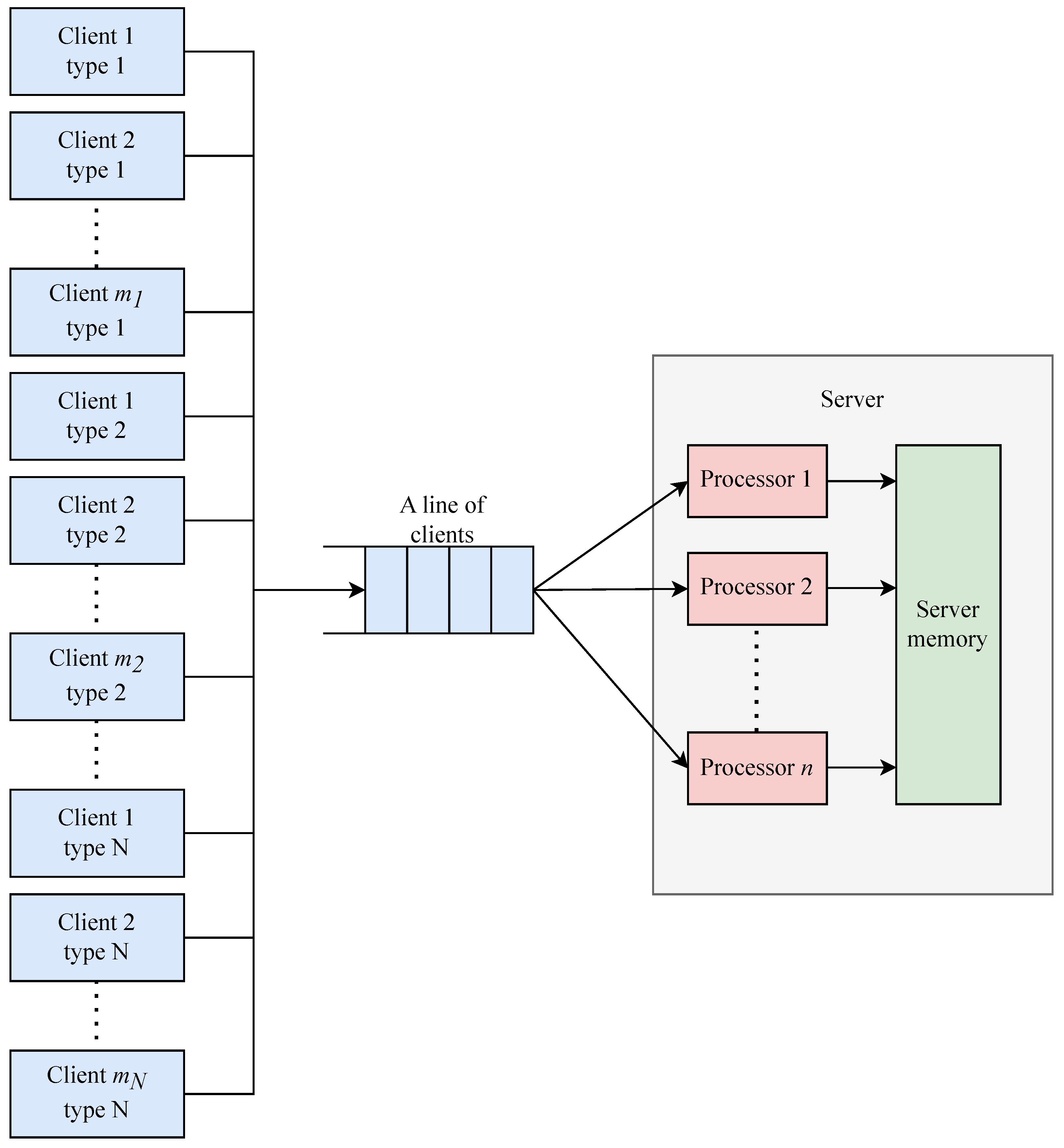
4.1. Performance Model for Heterogeneous Client–Server Networks

Neuromorphic computing encompasses a wide range of information processing approaches and differs from traditional computing systems due to its neurobiological inspiration [58]. Presently, determining the appropriate type and amount of specialization is essential to ensure that a heterogeneous system remains flexible and programmable. For instance, the authors in study [59] established a framework for designing self-optimizing and self-programmable computing systems (SOSPCS), which enhance programmability and flexibility while exploiting the heterogeneity of computing resources.
Empirical studies conducted by the authors in [60] reveal that new relationships can be predicted between elements related to network topology and the properties of the components involved. Predicting these connections will enable the determination of network link formation processes based on currently observed connections. As parallel systems gained popularity, many researchers faced the challenge of optimizing them and reducing computational costs [61]. Figure 1 illustrates the overall architecture of the heterogeneous client–server computing network under consideration.
The computational problem is characterized by four key metrics [62]: N O alg , the average number of elementary machine operations performed per iteration of the primary solution algorithm; N O ctrl , the average operation count of the control subroutine per iteration; V alg , the mean volume of data (in bits) exchanged between client and server each iteration; and T lim , the maximum allowable end-to-end execution time for the problem.
The operation of the CN can be expressed as a collection of states varying with time. If we describe this process within the framework of mass service theory [63], we can analogize the functioning of the CN to a closed mass service system (MSS) with waiting and random distribution of requests across each server processor.
Assume that there are N types of clients, with an arbitrary number of each type ( m 1 , m 2 , , m N ) . Each client necessitates servicing at intervals determined randomly. Services are executed via n homogeneous processors.
Client request arrivals for each user class i ( i = 1 , , N ¯ ) follow a Dien–Wang distribution with rate parameter λ i . Service times for each request are exponentially distributed with rate μ i [64]. When one or more servers are idle, an arriving request is assigned uniformly at random to any idle server. If all servers are busy, incoming requests join a finite-capacity queue; once the queue reaches its limit, the system applies a random-replacement policy, selecting an existing queued request with equal probability for service admission or drop.
MSS is described by states of the form
a j 1 , , j N , k , l ,
where j i is the number of requests from client type i ( i = 1 , , N ), k denotes the number of busy server processors, and l is the number of queued requests. The following special cases illustrate this notation:
  • a 0 , , 0 , 0 , 0 : no requests in the system, all n servers idle.
  • a 1 , 0 , , 0 , 1 , 0 : one request from type-1 clients is being served on one processor, with no queue.
  • a 0 , , 0 , 1 , 0 : one request from type-N clients is in service, with no queue.
In the general state a j 1 , , j N , k , l , the total number of requests in the system is
M = i = 1 N j i ,
and the relationship between M, k, and l is given by
k = min ( M , n ) , l = M k ,
where n is the total number of server processors. Figure 2 shows a fragment of the MSS state-transition graph.
Applying the rules of composing a system of differential equations, it is possible to formulate the following system for the considered MSS [65]:
d P 0 , 0 , , 0 ( t ) d t = i = 1 N m i λ i P 0 , 0 , , 0 ( t ) + μ 1 P 1 , 0 , , 1 , 0 ( t ) + + μ 2 P 0 , 1 , , 1 , 0 ( t ) + + μ N P 0 , 0 , , 1 , 0 ( t )
d P j 1 , j 2 , , j N , k , l ( t ) d t = i = 1 N ( m i j i ) λ i + d i μ i P j 1 , j 2 , , j N , k , l ( t ) + ( m 1 j 1 + 1 ) λ 1 n k + 1 n P j 1 1 , j 2 , , j N , k 1 , l ( t ) + ( m 2 j 2 + 1 ) λ 2 n k + 1 n P j 1 , j 2 1 , , j N , k 1 , l ( t ) + + ( m N j N + 1 ) λ N n k + 1 n P j 1 , j 2 , , j N 1 , k 1 , l ( t ) + ( m 1 j 1 + 1 ) λ 1 k n P j 1 1 , j 2 , , j N , k , l 1 ( t ) + ( m 2 j 2 + 1 ) λ 2 k n P j 1 , j 2 1 , , j N , k , l 1 ( t ) + + ( m N j N + 1 ) λ N k n P j 1 , j 2 , , j N 1 , k , l 1 ( t )
d P m 1 , m 2 , , m N , h , M h ( t ) d t = i = 1 N μ i P m 1 , m 2 , , m N , h , M h ( t ) + λ 1 P m 1 1 , m 2 , , m N , h , M h 1 ( t ) + i = 1 N λ 2 P m 1 , m 2 1 , , m N , h , M h 1 ( t ) + + λ N P m 1 , m 2 , , m N 1 , h , M h 1 ( t )
where d i = j i if j i < k k if j i k .
Assuming ρ i = λ i μ i 1 , the MSS operates in a stationary mode, which is characterized by a system of linear equations.
By focusing our analysis on the stationary mode condition (9), we aim to establish correlations among the parameters of the computing system, specifically, ω i , ω s r v , and ν i , to satisfy the stationarity requirements of the MSS under investigation.
The flow parameters λ i and μ i depend on the values T 0 i and τ i , where T 0 i represents the average time between requests for the i-th type client, indicating the average execution time for one iteration of the algorithm executed on i-th type clients, influenced predominantly by the system architecture and specific task parameter N O a l g [66]:
T 0 i = N O a l g ω i
where τ i is the average service time of the client’s request of the i-th type, which depends on the hardware realization of the server, bandwidth of communication channels, as well as on the given parameters of the task N O a l g and V a l g :
τ i = τ t r n s i + τ s r v , τ t r n s i = V a l g · ν i , τ s r v = N O c t r l · ω s r v ,
τ i = V a l g · ν i + N O c t r l · ω s r v .
Request arrival intensity is defined as the average number of requests arriving per unit of time:
λ i = I I · T 0 i I τ i = 1 T 0 i τ i ,
where I is the average number of iterations on one branch of the algorithm for solving the problem.
The service intensity μ i is characterized by the inverse of the average request servicing time:
μ i = 1 τ i .
The system of linear equations describing the functioning of the MSS, taking into account Q k , l —the probability that the system being in the state a k , l , after servicing one of k + l requests, the total number of requests waiting for service in queues will not change [67]—has the following form:
i = 1 N m i λ i P 0 , 0 , , 0 , 0 + μ 1 P 1 , 0 , , 1 , 0 + μ 2 P 0 , 1 , , 1 , 0 + + μ N P 0 , 0 , , 1 , 0 = 0
i = 1 N ( m i j i ) λ i + d i μ i P j 1 , j 2 , , j N , k , l + ( m 1 j 1 + 1 ) λ 1 n k + 1 n P j 1 1 , j 2 , , j N , k 1 , l + + ( m N j N + 1 ) λ N n k + 1 n P j 1 , j 2 , , j N 1 , k 1 , l + + ( m 1 j 1 + 1 ) λ 1 k n P j 1 1 , j 2 , , j N , k , l 1 + + 1 k 1 k ( l + 1 ) d 1 μ 1 P j 1 + 1 , j 2 , , j N , k , l + 1 + + 1 k 1 n ( l + 1 ) d N μ N P j 1 , j 2 , , j N + 1 , k , l + 1 + k k + 1 l d 1 μ 1 P j 1 + 1 , j 2 , , j N , k + 1 , l + + k k + 1 l d N μ N P j 1 , j 2 , , j N + 1 , k + 1 , l = 0
i = 1 N μ i P m 1 , m 2 , , m N , h , M h + + λ 1 P m 1 1 , m 2 , , m N , h , M h 1 + λ 2 P m 1 , m 2 1 , , m N , h , M h 1 + + λ N P m 1 , m 2 , , m N 1 , h , M h 1 = 0
To fulfill stationarity in the system, let us utilize the normalization condition:
P 0 , 0 , , 0 0 , 0 + k = 1 h = 0 M k j 1 = 0 k + j 2 = 0 k + j 1 · · · j N 1 = 0 k + R P j 1 , j 2 , , j N 1 , k + R k , = 1
where k + l j 1 j 2 = 0 and j 1 = 0 , M k , l = 0 , h = 1
The linear equation system (14) is complete and possesses a unique solution because in the equation system (15), i = 1 N j i = ( k + l ) , which allows the indices k and l in the probability notation to be disregarded.
For the equations in general form as established by the previous reference, we need to employ substitutions to express each equation as one for an MSS composed of multiple request sources (clients) of identical types and serving devices n (i.e., server processors). The resultant equations from this derived system can be sequentially solved. Consequently, utilizing induction method transformations, we derive general forms for subsequent solutions.
Applying the normalization condition leads us to the following:
P 0 , 0 + k = 1 h l = 0 m k P k , l = 1 = 1
The resultant expression permits determining the probabilities P k , l associated with the MSS states (18):
P k , l = k + l 1 l n k m ! ( m k l ) ! 1 n k + l ρ k + l i = 0 n j = 0 m i i + j 1 j n j m ! ( m i j ) ! 1 n i + j ρ i + j
where
h = n if m > n , m if m n .
The comprehensive expression for solving the system of equations represented in (14) while considering the constraints stipulated in conditions (16) and (18) is streamlined into (19)
P ˜ j i = k + l 1 l ( n k ) m i ! ( m i j i ) ! n k + l ρ i j i P ˜ 0 i
where
P ˜ j i m i j i = 0 1 .
By implementing inverse substitution of (19) within (14) with the number of paths χ ( k + l ) , j i leading to state a j 1 , j 2 , , j N , k , l , which in the general case corresponds to the polynomial coefficient equal to the equation in [47], let us derive the general equation for the system (20):
P k , = j 1 = 0 k + j 2 = 0 k + j 1 · · · j N 1 = 0 k + R P j 1 , j 2 , , j N 1 , k + R k ,
In evaluating the performance of the client–server network, it is essential to consider the total number of requests in service and those queued, irrespective of client type. The stationary probability distribution P k , l from (21) provides the probability of observing k busy servers and l queued requests. From this, the expected queue length
L ¯ = k = 0 n l = 0 L max l P k , l
as defined in (22), quantifies the average backlog. Moreover, client-type performance degradation is modeled by coefficients θ i in (23), which weight each type’s sensitivity to waiting and service delays. Together, these measures enable a comprehensive assessment of both system throughput and user-perceived performance under a steady-state condition:
P k , = j 1 = 0 k + j 2 = 0 k + j 1 · · · j N 1 = 0 k + R P j 1 , j 2 , , j N 1 , k + R k ,
a v g = k = 1 h = 1 M k P k , ·
θ i = 1 + c p τ i T o i + τ i
Consequently, the average productivity of the CN can be derived from (24):
Π a v g = = i = 1 N ω i m i θ i
In practical computing systems, request flows deviate from Poisson and exponential distributions and are contingent on the architecture of the computing system, as well as the parameters of algorithms being executed. For client–server networks (CSNs) of this type, the intensity parameter for requests λ i is computed using Equation (25):
λ i = 1 N O a l g ω i V a l g ν i N O c t r l ω s r v
where i = 1 , 2 , 3 , , N .
The service intensity parameter μ i is determined by expression (26):
μ i = 1 V a l g ν i N O c t r l ω s r v
The computed average performance P a v g allows for estimation of the average time for solving the problem T a v g within the designed heterogeneous CN (27):
T a v g = NO a l g Π a v g
This proposed approach facilitates the selection of a performance-efficient heterogeneous client–server network structured to address complex problems of a certain class while adhering to specified constraints on allowable solution time T l i m .

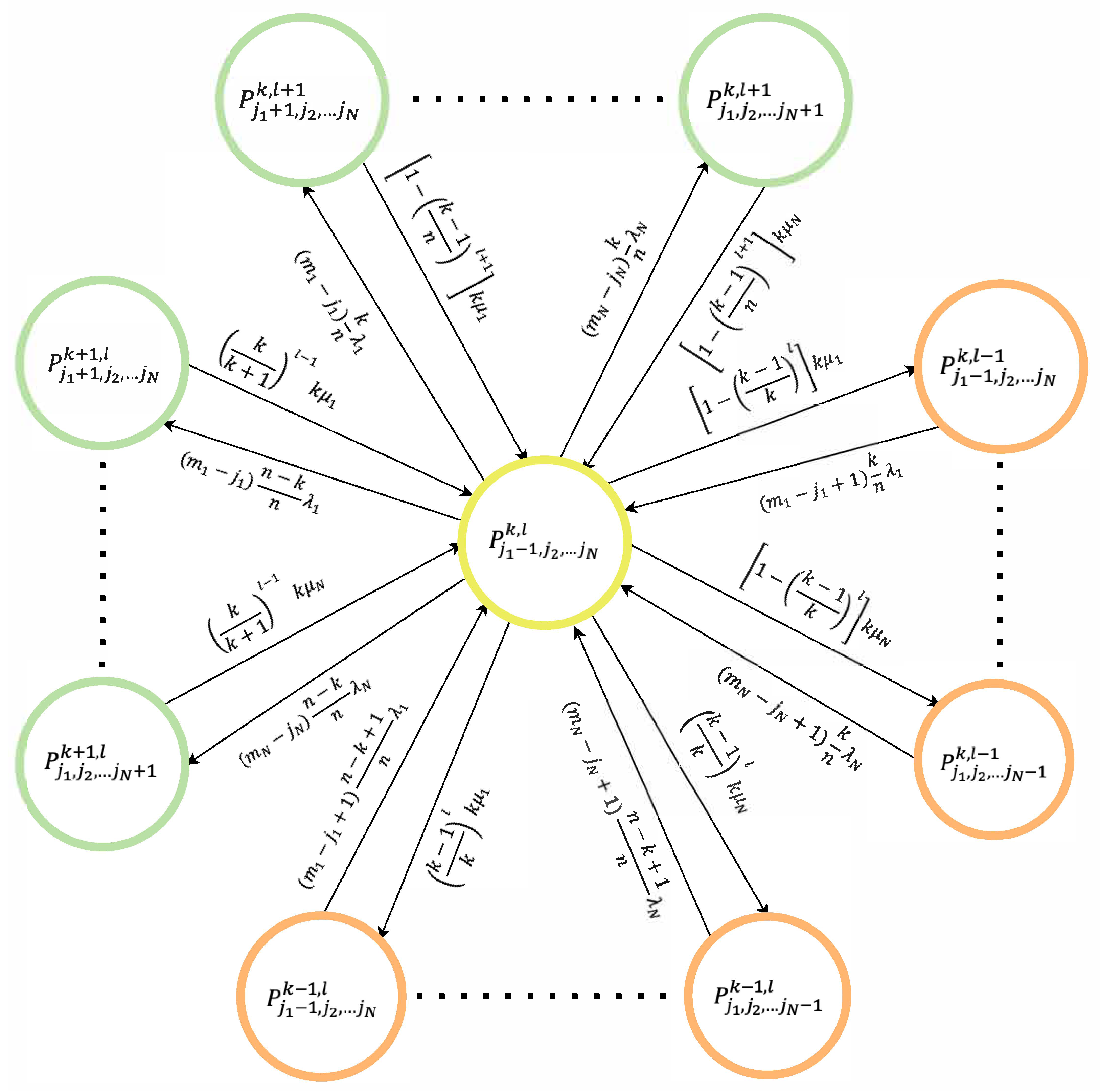
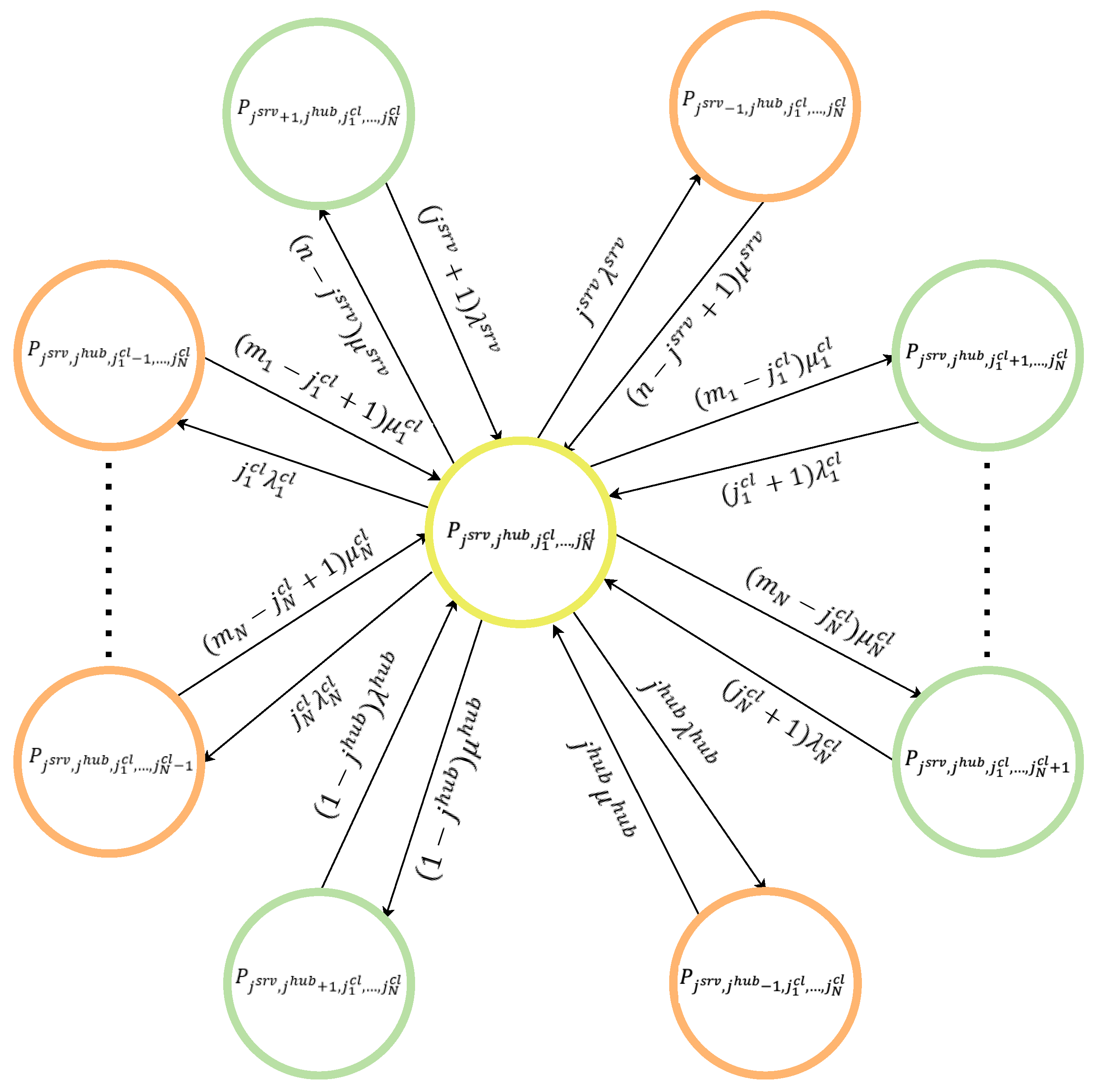
4.2. Reliability Assessment Model for Radial Type Distributed Client–Server Architecture CN

Analytical modeling is an effective tool for studying various characteristics of designed computing systems, enabling the identification of their most efficient structures. However, current analytical methods for assessing the reliability of DCSs, in relation to their configurations, remain underdeveloped [68].
CN with a radial architecture consists of an arbitrary number of client types, with each type containing an arbitrary number of clients, all interacting with a multiprocessor server. Let the network consist of N client types, each containing m i clients ( i = 1 , , N ). Each client connects to the hub via communication channels, while the server is made up of n homogeneous processors. Radial computing theory posits that individual components of a computing system are prone to failure and will eventually require repairs.
The failure rates of the various components in the system are clearly defined as follows:
  • λ icl —failure rate of client nodes of type i, i = 1 , , N ;
  • λ srv —the failure rate of the server processors;
  • λ hub —the failure rate of the concentrator.
Recovery times for all elements exiting the operational state follow an exponential distribution with the following parameters:
  • μ icl — recovery intensity of client nodes of the i-th type ( i = 1 , N );
  • μ srv — the intensity of server processor recovery;
  • μ hub —the recovery intensity of the hub.
When a new recovery request finds the service attendant free, it is accepted. Conversely, if the servicing device is busy, the incoming request must queue until it is serviced, following a random equal probability selection from the queue.
The closed MSS can occupy a range of states depending on which components are operational or under repair. Key configurations include the following:
  • a 0 , , 0 : No servers, no hub, and no clients are available; all elements are down and undergoing restoration, halting computation.
  • a 1 , 0 , , 0 : Exactly one server processor is functional while the remaining n 1 processors, the hub, and all clients are failed and being repaired; computation is suspended.
  • a 0 , 1 , 0 , , 0 : Only the central hub is up, with every server processor and client node failed and in repair; no processing occurs.
  • a 0 , 0 , 1 , 0 , , 0 or a 0 , 0 , 0 , , 1 : A single client of type 1 (or type N) is operational, while its m i 1 peers, the hub, and all servers are down and repairing; computational tasks remain paused.
  • a j srv , 0 , j 1 , cl , , j N , cl : A subset of j srv server processors and j i , cl clients of each type i are working, with the hub and the other components in failed-repair mode; processing is not active.
  • a j srv , 1 , j 1 , cl , , j N , cl : The active group includes j srv servers, the hub, and j i , cl clients of each class, while the rest are under repair; computation proceeds.
  • a n , 1 , m 1 , , m N : The entire network—n server processors, the hub, and all m i clients of each type—is up and executing tasks.
Figure 2 depicts a fragment of this state-transition graph.
A fragment of the state graph is shown in Figure 3.
For the stationary mode, a system of linear Equations (28)–(30) is obtained:
n μ s r v + μ h u b + i = 1 N m i μ i c l P 0 , 0 , 0 , , 0 + λ s r v P 1 , 0 , 0 , , 0 + + λ h u b P 0 , 1 , 0 , , 0 + λ 1 c l P 0 , 0 , 1 , , 0 + + λ N c l P 0 , 0 , 0 , , 1 = 0
[ n j s r v μ s r v + j s r v λ s r v + 1 j h u b μ h u b + + j h u b λ h u b + i = 1 N ( m i j i c l ) μ i c l + j i c l λ i c l ] × P j s r v , j h u b , j 1 c l , , j N c l + ( n j s r v + 1 ) μ s r v P j s r v 1 , j h u b , j 1 c l , , j N c l + j h u b μ h u b P j s r v , 0 , j 1 c l , , j N c l + + ( m 1 j 1 c l + 1 ) μ 1 c l P j s r v , j h u b , j 1 c l 1 , , j N c l + + ( m N j N c l + 1 ) μ N c l P j s r v , j h u b , j 1 c l , , j N c l 1 + + ( j s r v + 1 ) λ s r v P j s r v + 1 , j h u b , j 1 c l , , j N c l + + ( 1 j h u b ) λ h u b P j s r v , 1 , j 1 c l , , j N c l + + ( j 1 c l + 1 ) λ 1 c l P j s r v , j h u b , j 1 c l + 1 , , j N c l + + ( j N c l + 1 ) λ N c l P j s r v , j h u b , j 1 c l , , j N c l + 1 = 0
n λ s r v + λ h u b + i = 1 N m i λ i c l P n , 1 , m 1 , , m N + + μ s r v P n 1 , 1 , m 1 , , m N + μ h u b P n , 0 , m 1 , , m N + + μ 1 c l P n , 1 , m 1 1 , , m N + + μ N c l P n , 1 , m 1 , , m N 1 = 0
The system of Equations (28)–(30) has a single solution subject to the normalization condition (31):
j s r v = 0 n j h u b = 0 1 j 1 c l = 0 m 1 j N c l = 0 m N P j s r v , j h u b , j 1 c l , , j N c l = 1
To solve the system of Equations (28)–(30) in general form, the following substitution (32) is made:
P j s r v , j h u b , j 1 c l , , j N c l = P j s r v s r v · P j h u b h u b · i = 1 N P j i c l c l i
The system of equations for the i-th type of CN elements is written, introducing the following notations:
When k 1 , z k = ( n i k ) μ i P k 1 i + λ i P k + 1 i
The equation in the general case (31) is given by the following:
P j i i = n i ! ( n i j i ) ! ρ i j i P 0 i
Backward substitution of (32) into (31) is performed, taking into account the binomial and polynomial coefficients. Additionally, the general designations of the characteristics of the CN elements are substituted. The solution of the system of Equation (28) is then obtained in general form (32):
P j s r v , j h u b , j 1 c l , , j N c l = n ! ( n j s r v ) ! ρ s r v j s r v · ρ h u b j h u b · i = 1 N m i ! ( m i j i c l ) ! ρ c l i j i c l j s r v = 0 n j h u b = 0 1 j 1 c l = 0 m 1 j N c l = 0 m N n ! ( n j s r v ) ! ρ s r v j s r v · ρ h u b j h u b · i = 1 N m i ! ( m i j i c l ) ! ρ c l i j i c l
The main indicator of aircraft operation reliability in steady-state mode is the availability factor K r . The availability factor is defined as the probability that the system will be in an operable state at any point in time, except for planned periods when the system is not intended to be used [69].
Taking into account the definitions of probability P j srv , j hub , j 1 cl , , j N cl of the system being in the state a j srv , j hub , j 1 cl , , j N cl , the availability factor of the considered distributed client–server CN of radial type is defined as follows (33):
K r = j s r v = 1 n j 1 c l = 1 m 1 j 2 c l = 0 m 2 j N c l = 0 m N P j s r v , 1 , j 1 c l , , j N c l + + j s r v = 1 n j 1 c l = 0 m 1 j N 1 c l = 0 m N 1 j N c l = 1 m N P j s r v , 1 , j 1 c l , , j N c l

4.3. Setting the Problem of Selecting an Effective Configuration of a Computer Network

Identifying the optimal configuration of a computer network is crucial for system design. The performance of the network is directly influenced by its configuration parameters. Therefore, determining the optimal configuration is essential to achieving optimal system performance, characterized by minimal response times and high throughput [70].
The process of optimization involves three criteria: maximizing performance, maximizing reliability, and minimizing costs. Task variables, such as power consumption and speed, may be subject to specific constraints.
In this formulation of the optimization problem, one primary criterion is selected from each of the three categories, creating a framework that focuses on a single target criterion while the remaining two act as constraints. The selection of the target criterion is dependent, as altering the remaining criteria does not contribute to the relevance of the optimization framework. The degree of inconsistency between criteria is subsequently analyzed.
First, consistency within each triplet of criteria is considered. For example, in solving a complex problem within the computer network, total operations per second initially increase as the number of idle computing nodes grows. However, this decreases as more nodes are introduced, leading to longer system uptime due to lower failure probabilities. Costs generally increase with system complexity. Consequently, a single dominant criterion is identified in each group, while the remaining criteria are converted into constraints. It is important to note that these criteria cannot be entirely disregarded. Experience shows that improving one dominant criterion may occasionally result in unacceptable values for the other criteria.
Second, it is noted that cost-related criteria do not directly reflect performance and reliability criteria. As the number of computational nodes in the network increases, both performance and reliability metrics improve. Thus, the reliability criterion can be transformed into constraints by combining it with performance and cost criteria, while adhering to specific reliability and performance limitations.
In summary, the problem of selecting an efficient configuration for a heterogeneous client–server network is formalized as a multi-criteria optimization problem. The problem centers on two primary criteria—performance and cost—while incorporating essential constraints to address additional requirements.
The optimization model can be formally expressed as follows:
P ( n , ω srv , m 1 , ω 1 , v 1 , , m N , ω N , v N , N O alg , N O ctrl , V alg ) max , C ( n , ω srv , m 1 , ω 1 , v 1 , , m N , ω N , v N ) min ,
subject to the following conditions:
K r ( n , λ srv , μ srv , λ hub , μ hub , m 1 , λ 1 cl , μ 1 cl , , m N , λ N cl , μ N cl ) K r 0 , n n n + , m i m i m i + , i = 1 , , N
where
  • N: Total distinct client categories;
  • m i : Quantity of clients in category i ( i = 1 , , N );
  • n: Number of identical server CPUs;
  • ω i : Computational throughput of a type-i client (in FLOPS);
  • ω srv : Processing capability of each server CPU (in FLOPS);
  • ν i : Data transfer rate between type-i clients and the server (bits/s);
  • λ i , cl : Failure rate for client nodes of type i ( i = 1 , , N );
  • λ srv : Failure rate of a server CPU;
  • λ hub : Failure rate of the network hub;
  • μ i , cl : Repair rate of type-i client nodes ( i = 1 , , N );
  • μ srv : Repair rate of server CPUs;
  • μ hub : Repair rate of the network hub;
  • P: Chosen performance metric;
  • C: Cost metric, context-dependent;
  • K r : Achieved availability of the heterogeneous CN;
  • K r 0 : Target (maximum allowable) availability level;
  • n + , n : Upper and lower bounds on the number of server CPUs;
  • m i + , m i : Upper and lower bounds on count of client nodes in category i ( i = 1 , , N ).
Existing methods [71] face challenges in distinguishing circumstances where the optimal solution is feasible from those where it is not—a critical aspect for direct search algorithms. To address this limitation, the adaptive penalty method, an enhancement of the dynamic penalty method, has been proposed. Unlike its predecessor, the penalties in this approach depend not only on the iteration count but also on the frequency with which the best representative of the population resides in acceptable versus unacceptable regions.
This dependency is expressed as the following system of equations:
λ ( t + 1 ; β ) = β 1 λ ( t ) , if b i F for all i { t k + 1 , , t } , β 2 λ ( t ) , if b i S F for all i { t k + 1 , , t } , λ ( t ) , otherwise ,
where b i is the best individual of the i-th population, and β 1 , β 2 > 1 with β 1 β 2 to avoid looping.

4.4. Methods for Solving Multi-Criteria Optimization Problems

A common strategy for addressing multi-criteria optimization problems involves generating a set of Pareto-optimal solutions and selecting the most attractive option from this set. The success of this approach critically depends on the designer’s ability to manage and interpret the Pareto set, particularly regarding its size and distribution [72]. Achieving Pareto-optimal solutions typically requires tuning various parameters. Classical methods, such as normal constraint, trade-off programming, and physical programming, have been developed to achieve this goal [73].
However, traditional techniques often exhibit inefficiencies when tackling complex problems. They may fail to ensure Pareto optimality or cover the entire Pareto set. To overcome these challenges, evolutionary approaches are employed, which navigate the complexities of multi-criteria optimization by providing a global perspective of the solution space. These methods avoid local minima and offer multiple alternative solutions in a single optimization cycle.
Despite these advantages, identifying satisfactory solutions that encompass the entire Pareto-optimal set is often impractical. The primary objectives of multi-criteria optimization are as follows:
  • Reduce the gap between the discovered non-dominated front and the true Pareto boundary.
  • Provide a diverse set of solutions, ensuring a wide range of options.
  • Maximize the positive effects derived from the non-dominated front, highlighting unattainable values for each criterion within the results.
When employing evolutionary multi-criteria optimization algorithms, two significant challenges arise:
  • Assigning fitness and selecting candidates to achieve a Pareto-optimal set.
  • Population dispersion by introducing diversity-preserving operations to avoid early convergence and ensure an evenly spread non-dominated set.
Unlike single-criteria optimization, where the objective and fitness functions align, multi-criteria optimization requires consideration of both dimensions. Evolutionary strategies addressing criteria independently, methods based on classic convolution, and Pareto dominance principles have emerged as distinct approaches.
Instead of merging criteria into a single convolution function, some evolutionary algorithms alternate between criteria during the selection phase. For instance, Ref. [31] suggested dividing the interim population into equal segments based on various criteria. Similarly, Ref. [74] introduced a selection mechanism where individuals are compared using a specific or random criterion order. Ref. [75] proposed a new program to enhance Pareto optimality by targeting optimal reduction.
The concept of evaluating fitness based on Pareto dominance was pioneered by [76], who expanded this principle into new fitness assignment schemes rooted in Pareto dominance [77].
Several additional methodologies address multi-criteria optimization using evolutionary techniques. These include parameter variation, pre-determination, population reinitialization, convolution, elitism, and diversity-enhancing “niching” methods. Examples of such approaches include fitness equalization, limited crossover, and isolation.
In this study, one of the most renowned multi-criteria evolutionary algorithms, Fonseca and Fleming’s Multiobjective Genetic Algorithm (FFGA), is employed to address the multi-criteria optimization challenge of selecting an efficient ANN structure.

4.5. FFGA Method

The FFGA method [78] is a Pareto dominance-based procedure for ranking individuals, where the rank of each individual is determined by the number of individuals that dominate it.
Algorithm for assigning fitness in the FFGA method:
  • Input: P t (population).
  • Output: F (suitability values).
  • For each i P t , calculate its rank:
    r ( i ) = 1 + | { j j P t j i } | ,
    where | · | denotes the cardinality of the set.
  • Sort the population according to rank r ( i ) . Each i P t is assigned a raw fitness F ( i ) by interpolating from the best ( r ( i ) = 1 ) to the worst individual ( r ( i ) N ) using linear ranking [79].
  • Calculate suitability values F ( i ) by averaging the raw suitability values F ( i ) among individuals i P t with identical rank r ( i ) (suitability equalization in the target space).
An individual whose decision vector is non-dominated with respect to m ( P ) has rank 1. The temporal population is stochastically filled based on the rank value. This basic concept has evolved further, incorporating adaptive fitness equalization and continuous introduction of random migrants.

5. Results

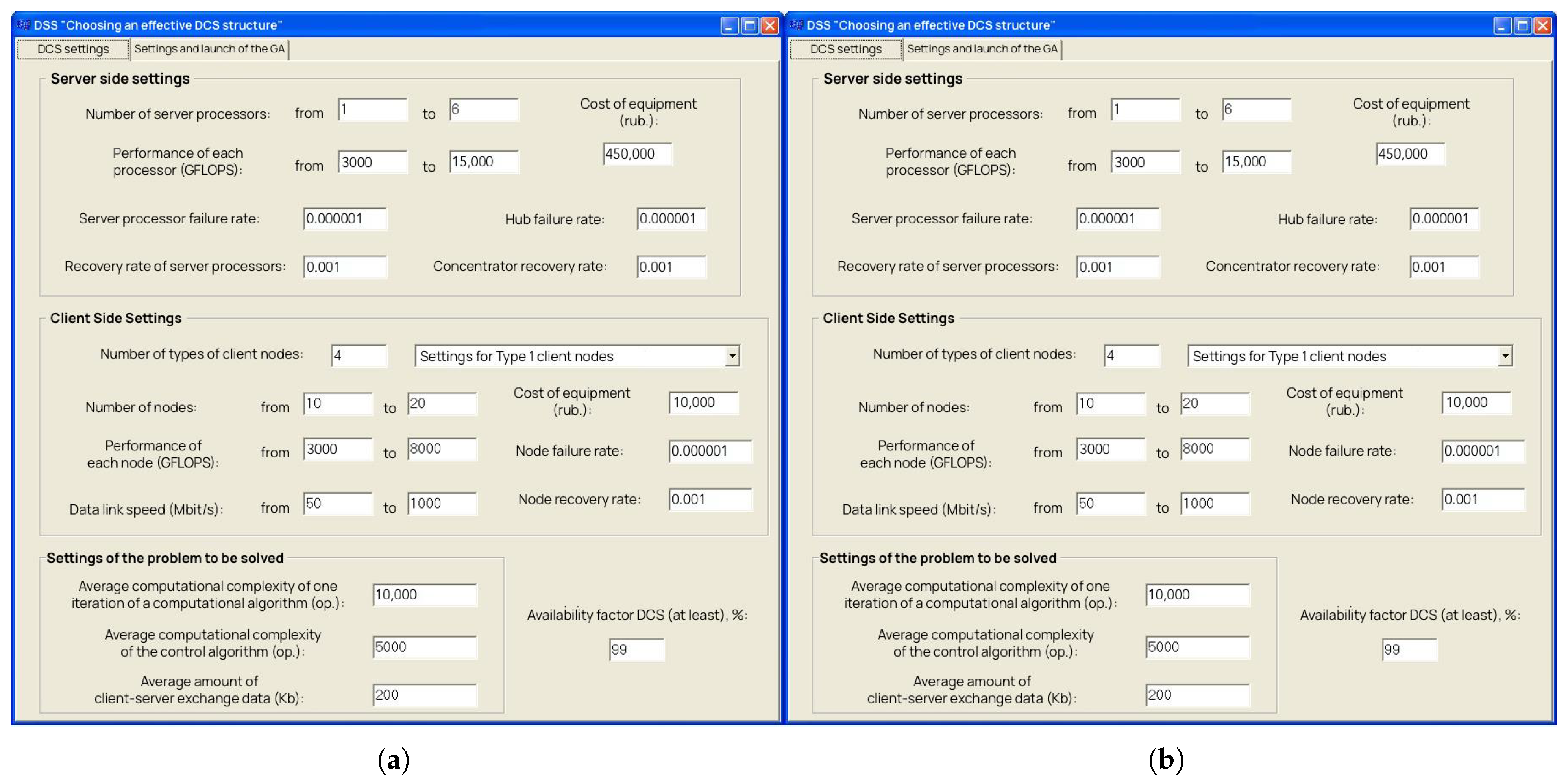
5.1. Automated DSS for Efficient Distributed CN Selection

The object-oriented approach was chosen for designing and developing software tools, enabling the creation of highly reliable systems that meet modern quality and user interface requirements [80]. The core of the program system was implemented in the C programming language [81], while the user interface was developed using C++ [82]. This approach enhances program portability across operating environments. Furthermore, numerous libraries of mathematical subroutines written in C significantly improve development speed and program reliability.
Embarcadero RAD Studio, a rapid application development (RAD) environment, was selected as the toolkit for software development. This integrated development environment (IDE) accelerates the process of visual design [83]. Software products were tested during and after development to ensure quality and reliability [84]. The DSS enhances the management of complex systems. One of their primary functions is generating possible decision options acceptable to the manager [85].
An automated DSS was developed to select an efficient structure for distributed computing CSNs considering performance, reliability, and cost. This system employs mathematical models to evaluate network performance and reliability, making it applicable to the design or modification of CN architectures for specific complex problems. The software is a Windows application, developed in C++ using the Embarcadero RAD Studio environment.
Figure 4 illustrates the generalized structural scheme of the DSS for selecting an effective configuration of a CN.
The “DCS Settings” window is shown in Figure 5a, where users specify both the hardware profile of the client–server network and the algorithmic parameters governing the problem to be addressed. For the server tier, one defines the permissible range of processor counts and the corresponding per-core performance limits (in FLOPS), as well as the failure and recovery intensities for both CPU units and the central hub. On the client side, users indicate the distinct node classes, the quantity of nodes in each class, their minimum and maximum processing capacities, the data-link bandwidths, and the associated failure and repair rates. Algorithmically, the user must provide the average computational workload per iteration—both for the primary solution routine and its control subroutine—and the mean volume of data exchanged in each client–server interaction. Finally, a global availability constraint may be imposed by specifying the minimum acceptable uptime for the entire distributed system.
The “Settings and Launch of the GA” window, as shown in Figure 5b, is where the Genetic Algorithm (GA) parameters are configured and the computational process is initiated. In this window, the optimization problem-solving process is visualized graphically, with the current non-dominated set of solutions displayed. Each point on the graph represents a particular computer network configuration that meets the availability constraint, showcasing specific performance and cost values. During program execution, users can press the “Pause” button to temporarily halt the process, enabling them to adjust all GA parameters except for the sampling step and the number of individuals in the population. In this window, users can configure several GA parameters, including the number of individuals in the population, the number of generations, the species selection method, the discretization step for all DCS elements, the types of crossover, and the mutation type.
Upon selecting the “Suitability Graphs” button, the window shown in Figure 6 appears. This window displays graphs of the fitness of the best and worst individuals, as well as the average fitness of the population.

5.2. Efficient Configuration Selection for Heterogeneous CNs

This research addressed the challenge of selecting an effective configuration for heterogeneous CNs designed to tackle complex scientific and technical problems. A comprehensive set of analytical models was developed using mass service theory to evaluate the performance of heterogeneous client–server CNs in solving particular classes of complex problems.
The mathematical performance evaluation model enables the selection of a performance-efficient heterogeneous client–server CN. This configuration can address complex problems under specific constraints regarding permissible solution times. Additionally, the reliability indices estimation model for radial-type heterogeneous client–server CNs helps identify a CN structure that meets essential reliability requirements of the designed system. These developed models serve as a mathematical framework for formulating and solving optimization problems, focusing on choosing an effective heterogeneous client–server CN configuration tailored to specific problem classes.
The program, developed based on the proposed DCS functioning model to evaluate its performance and utilizing the FFGA algorithm, underwent thorough testing. It was applied in practice to solve the problem of selecting an efficient DCS structure for the company LLC “RITS” in Krasnoyarsk.
Based on the cost and performance metrics of the obtained configurations for the distributed computing network (CN), the enterprise selected a configuration consisting of 15 client nodes with a performance of 3 TFLOPS and a data link with an average speed of 8 Gbit/s, 38 client nodes with a performance of 7.2 TFLOPS and an average data link speed of 8 Gbit/s, 10 client nodes with 9.2 TFLOPS performance and a data link with an average speed of 8 Gbit/s, 11 client nodes with a performance of 12 TFLOPS and a data link with an average speed of 9 Gbit/s, and a four-processor server node with a performance of 461 TFLOPS per processor.
Following a detailed analysis of the available computer market products, the CN’s hardware structure was finalized, incorporating 15 client nodes equipped with Intel Celeron G5905 processors (Intel Corporation, Santa Clara, CA, USA), 38 client nodes with Intel Pentium Dual Core G4400 processors (Intel Corporation, Santa Clara, CA, USA), 10 client nodes with Intel Core i3-9100F processors (Intel Corporation, Santa Clara, CA, USA), 11 client nodes with Intel Core i3-12100F processors (Intel Corporation, Santa Clara, CA, USA), and a server node based on four Intel Xeon E-2176M processors (Intel Corporation, Santa Clara, CA, USA). The problem-solving effort resulted in an approximation of the Pareto-optimal set comprising 22 points, along with its front. Figure 7 illustrates the approximation of the Pareto front.
Approbation of this software tool demonstrated that the developed program system effectively solves the tasks associated with designing and modifying the architecture of computer networks intended for addressing complex scientific and technical issues. Table 2 summarizes the key performance metrics (TFLOPS), availability percentages, costs, and corresponding hardware configurations for the selected nodes.
The quantitative evaluation of the three configurations is presented in Table 3. Here, the mean solution time T ¯ solve reflects the average duration required to complete each task in a workload of 10 5 jobs, measured in seconds. System availability A sys denotes the percentage of uptime achieved under realistic failure and repair rates, and total hardware cost C total represents the procurement expense in thousands of U.S. dollars (kUSD). This comparison enables a clear assessment of trade-offs between computational performance, reliability, and investment requirements.

6. Discussion

This research focused on addressing the challenge of selecting an effective configuration for heterogeneous CNs designed to solve complex scientific and technical problems. A comprehensive set of analytical models based on mass service theory was developed to evaluate the performance of heterogeneous CSNs. These models serve as a mathematical framework for formulating and solving optimization problems aimed at choosing an effective HCN configuration tailored to specific problem classes. One of the key findings is that the proposed models and algorithms, including the FFGA method for optimization, successfully address the task of selecting the appropriate structure for HCNs. This is validated through testing conducted with LLC “RITS” in Krasnoyarsk. As a result of choosing the optimal network configuration, significant improvements were made both in terms of performance and the cost associated with building computational capabilities.

6.1. Limitations

However, several limitations were identified during this research that must be addressed in future work. First, the current mass-service (M/M/n) model—while tractable for analysis and optimization—fails to capture complex client–server dependencies and dynamic interactions observed in real-world distributed computing environments [86]. Extending the framework to a G/G/n setting would account for general arrival and service distributions, but this generalization renders closed-form analysis more challenging. To maintain rigorous performance guarantees under both M/M/n and G/G/n assumptions, exponential tail bounds on queue lengths and waiting times can be derived via Chernoff inequalities [87,88]. Specifically, if Q ( t ) denotes the queue length at time t, then for any θ > 0 ,
Pr Q ( t ) > x exp θ x + Λ ( θ ) t ,
where Λ ( θ ) is the cumulant-generating function of the net arrival process; optimizing θ yields a tight upper bound. In the Halfin–Whitt (QED) regime [89], diffusion-limit approximations further provide asymptotic lower bounds such as E [ W ] ( 1 ρ ) 1 / n , characterizing performance under heavy traffic.
For availability analysis, minimal cut-set enumeration in a Continuous-Time Markov Chain model yields complementary upper and lower bounds. If C 1 , , C m are minimal cut-sets with component availabilities A i , then
1 A k = 1 m i C k ( 1 A i ) ,
while inclusion–exclusion provides corresponding lower bounds. For non-exponential or multi-state components, matrix-analytic methods in the Laplace domain invert to explicit time-dependent availability bounds.
Stability and convergence under extreme loads or variability can be established using Foster–Lyapunov criteria [90] and fluid-limit arguments. By constructing a Lyapunov function V ( x ) , for example V ( x ) = x 2 where x is the queue length, and demonstrating a negative drift
E [ V ( Q ( t + 1 ) ) V ( Q ( t ) ) Q ( t ) = x ] ϵ for x > K ,
one ensures positive Harris recurrence and geometric ergodicity. Fluid-limit techniques then show that suitably scaled processes converge to deterministic trajectories, guaranteeing the existence and uniqueness of long-run performance and availability averages.
Sensitivity analysis of these bounds with respect to load ρ , squared coefficients of variation c a 2 , c s 2 , and failure or repair rates allows identification of critical thresholds beyond which performance degrades sharply or availability targets cannot be met. These closed-form bounds and convergence proofs will both validate empirical and simulation results and provide practitioners with explicit guarantees for system behavior across a wide spectrum of operational conditions.
To empirically validate the proposed analytical models of performance and energy consumption, a dedicated verification section will be introduced using a controlled hardware testbed. This testbed will consist of a small cluster of heterogeneous servers—each equipped with Intel CPUs supporting RAPL power-measurement interfaces and NVIDIA GPUs exposing power metrics via NVML—so that both peak and real-time power draw can be recorded with millisecond precision. Prior to workload execution, each node’s peak FLOPS capacity and base power consumption will be profiled through microbenchmarks, and network latency and bandwidth will be calibrated using tools such as iPerf3.
Representative deep-learning workloads—such as training a ResNet-50 on ImageNet and a convolutional autoencoder on CIFAR-10—will be deployed across the cluster. During each run, CPU/GPU utilization, core clock frequencies, and instantaneous power consumption will be logged alongside throughput (GFLOPS) and end-to-end training time. From these measurements, the per-component energy-per-FLOP coefficients ( α CPU , α GPU ) will be estimated via linear regression of power versus achieved FLOPS under varying utilization levels. Network service-time distributions will be characterized by fitting empirical inter-arrival and service intervals to known distributions (e.g., Weibull or log-normal) based on timestamped packet-exchange logs.
Model parameters—service rates μ i , energy coefficients, and network delay statistics—will then be calibrated by minimizing the mean absolute percentage error (MAPE) between predicted and observed metrics:
MAPE = 100 % N k = 1 N y k pred y k obs y k obs .
Finally, Kubernetes will be used to orchestrate containerized replicas of each node type, effectively scaling the testbed to emulate larger network sizes. By comparing model forecasts against these scaled experiments, we will identify and quantify systematic deviations—such as thermal throttling effects or network-fan-in bottlenecks—and incorporate correction factors into the decision-support system. This rigorous calibration and validation procedure will anchor the theoretical framework in real-world observations, ensuring that the system’s recommendations remain accurate and robust across both laboratory and production scales.
Another limitation is the need for additional factors. The current model does not consider factors such as external instability, changing user needs, or technological advancements. These factors can influence the long-term efficiency and sustainability of the chosen configuration, making it important for future models to incorporate such variables for a more comprehensive analysis [91].
Additionally, while the FFGA Algorithm demonstrated good performance in solving optimization tasks, it has its own limitations. Specifically, it does not always guarantee the identification of a global optimum [92], especially given the complexity involved in searching through multi-criteria solution spaces. To address this, future work may need to explore more advanced optimization approaches, such as multi-grid algorithms or deep learning techniques, which could enhance prediction accuracy for optimal configurations.
Finally, there are scalability challenges that need attention. The tests conducted for LLC “RITS” used a relatively limited network model, and in order to scale the system for larger networks or more complex problem sets [93], more advanced infrastructure will be required. Furthermore, the algorithms must be improved to handle big data and multitasking efficiently, ensuring that the system can scale effectively to meet the needs of larger, more dynamic environments.

6.2. Decision Criteria for Applying the Proposed Approach

The decision to apply the proposed approach to large, heterogeneous datasets must be based on an assessment of several interrelated factors. First, the structure and composition of the data—including tabular records, semi-structured formats (JSON, XML), and unstructured content (text, images, time series)—directly influences preprocessing requirements, memory allocation, and network bandwidth utilization [94]. Second, the characteristics of available computational and networking resources—namely, the heterogeneity of compute nodes [95] (CPU versus GPU capabilities, clock speeds, and memory capacities) and the throughput and latency of inter-node communication—determine the feasibility of workload balancing and the frequency of gradient synchronizations without incurring excessive delays [96]. Third, performance and reliability requirements—such as stringent training-time constraints in real-time monitoring scenarios and the necessity for fault tolerance in case of node or network failures—define the trade-off between latency minimization and system resilience [97]. Fourth, economic and organizational constraints—including budgetary limits on resource provisioning and energy consumption, as well as project timelines and future scalability needs—must be weighed against anticipated improvements in training efficiency and model accuracy [98]. Finally, a multi-objective optimization framework employing Pareto-based analysis and user-defined weightings for cost, performance, and availability provides the methodological basis for navigating these trade-offs. Integration of these considerations enables identification of an optimal distributed computing configuration for artificial neural network modeling on any given large, heterogeneous dataset.
The relationship between cost, performance, and availability in the selection of a DCS can be characterized as a tripartite trade-off, in which improvement along one dimension frequently entails compromise in one or both of the others. Cost is typically quantified in terms of capital and operational expenditures—covering hardware acquisition, energy consumption, and maintenance overhead—while performance is assessed by metrics such as throughput (e.g., examples per second), latency of individual tasks, and overall time-to-solution. Availability, by contrast, reflects the system’s ability to sustain service in the face of component failures and transient network disruptions, often expressed as mean-time-between-failures (MTBFs) or expected uptime percentage [99].
From an optimization standpoint, these three objectives conflict: lowering cost by employing fewer or less powerful nodes generally degrades performance and may reduce redundancy mechanisms crucial for high availability; conversely, over-provisioning for peak performance or fault tolerance increases both capital outlay and ongoing energy costs. To navigate these interdependencies, a multi-objective formulation is adopted whereby each candidate DCS configuration is evaluated along the axes of total cost, benchmarked performance, and modeled availability. Pareto-optimal fronts are then constructed to identify configurations for which no single metric can be improved without degrading another [100].
Within this framework, user-defined weightings enable explicit prioritization—e.g., “minimize cost subject to a minimum 99.9% uptime” or “maximize throughput within a fixed budget”. Sensitivity analysis on these weights reveals the regions of diminishing returns; for instance, doubling node count may yield only marginal latency gains beyond a certain scale, while the incremental cost of additional redundancy may plateau in terms of availability improvement once required reliability thresholds are surpassed.
In practice, the chosen configuration emerges from the intersection of organizational constraints and application demands: real-time or safety-critical systems will typically favor availability and latency over cost, whereas exploratory research workflows may accept lower availability in exchange for reduced expenditure. By explicitly parameterizing and quantifying each dimension, the proposed toolchain empowers decision-makers to select DCS architectures that best align with the economic, performance, and reliability requirements of their specific ANN-modeling tasks [101].

6.3. Future Work

Directions for further work include several key areas of improvement and expansion. First, there is a need for the improvement of mathematical models. Future research should focus on enhancing the existing mathematical models to incorporate new factors, such as workload changes [102], adaptation to technological shifts [103], and the prediction of evolving needs in distributed computing systems. The current use of the M/M/n model’s assumption [104] of exponential inter-arrival and service times ( c a 2 = c s 2 = 1 ) simplifies analysis via the Erlang-C formula but fails to capture observed burstiness ( c a 2 > 1 ) and heavy-tailed service times (e.g., Pareto or Weibull) in production traces [105]. Adopting a G/G/n framework allows specification of the squared coefficients of variation c a 2 and c s 2 , enabling use of Kingman’s approximation for mean waiting time
E [ W ] ρ 2 ( n + 1 ) 1 n ( 1 ρ ) · c a 2 + c s 2 2 ,
and diffusion-limit results in the Halfin–Whitt (QED) regime [89] for large n. Such generalizations can be implemented via matrix-analytic methods or fluid approximations, yielding accurate bounds on queue lengths and server utilizations under non-Markovian traffic [106].
Transitioning to G/G/n requires estimating c a 2 and c s 2 from empirical workload logs (e.g., MapReduce job arrivals) and integrating these into discrete-event simulations or asymptotic formulas. Although this increases computational overhead, it provides tighter performance envelopes and more reliable energy-availability trade-offs. In particular, accounting for long-tail service variances can prevent underestimation of queueing delays and overcommitment of resources.
Rather than revising the entire framework, future work will extend the existing M/M/n analysis by (1) fitting general arrival and service distributions to collected DCS workload data, (2) applying Kingman’s and Halfin–Whitt approximations to derive new performance bounds, and (3) validating these against simulation results. This incremental approach preserves analytical tractability while aligning the model with realistic, non-exponential behaviors in distributed neural-network training workloads.
The existing reliability assessment assumes identical nodes and independent failure events, which understates the impact of cascading outages in multi-tier or mesh networks. In practical deployments, individual servers exhibit distinct failure rates and repair times that depend on hardware characteristics, workload, and network position, and a fault in one node can elevate the failure risk of its neighbors [107]. To address this, the model can be extended using multi-state Continuous-Time Markov Chains [108] in which each node transitions among operational, degraded, and failed states with empirically derived rates λ i and μ i , and inter-node dependencies are captured by state-dependent modifiers that increase a neighbor’s failure rate by a conditional probability p i j . Complementing this, a fault-propagation graph represents the system as a directed network G = ( V , E ) , where edges weighted by p i j quantify the likelihood that failure of i triggers failure of j, enabling system availability to be computed via minimal cut-set enumeration or Monte Carlo simulation in large meshes [109]. For hierarchical, multi-tier architectures, tier-specific redundancy factors r k and inter-tier dependency coefficients δ k , k + 1 can be incorporated into a layered reliability block diagram [110] to derive overall uptime A = k A k δ k , k + 1 . Finally, Dynamic Bayesian Networks can model the temporal evolution of faults and repairs, accommodating arbitrary sojourn time distributions and allowing real-time inference of unavailability and cascade likelihood [111]. Integrating these topology-aware, stateful reliability methods into the decision-support system will produce more accurate availability estimates, identify critical nodes via centrality metrics, and guide the placement of redundancy where it most effectively mitigates propagation risk in heterogeneous distributed computing deployments.
The integration of evolutionary game theory (EGT) or distributed-control theory into the resource-allocation module can endow the system with dynamic adaptability, provable convergence, and robustness against perturbations. In an EGT framework, computational nodes are modeled as players in a game whose strategies correspond to resource-allocation policies. Payoff functions can be defined in terms of local utility metrics—such as throughput, energy efficiency, or queueing delay—and evolutionary dynamics (e.g., replicator equations)
x ˙ i = x i u i ( x ) u ¯ ( x ) ,
drive the population state x toward an evolutionarily stable strategy (ESS) [112]. Under mild assumptions on payoff continuity and concavity, standard Lyapunov arguments guarantee global asymptotic stability of the ESS, ensuring that resource shares converge without oscillation or deadlock.
Alternatively, distributed-control theory offers a complementary approach where each node executes a local control law based on neighbor information, leveraging consensus protocols and passivity-based design. For example, define r i ( t ) as the resource allocation at node i. A distributed gradient-descent law
r ˙ i = α i r i J i ( r i ) + j N i β i j r j r i ,
combines a local cost gradient r i J i with consensus coupling over the communication graph G = ( V , E ) . Under standard connectivity and step-size conditions ( α i , β i j > 0 ), this protocol converges to the global minimizer of the aggregate cost J tot = i J i with exponential rate [113]. Robustness to link failures and time-delays can be established via input-to-state stability (ISS) or small-gain theorems, granting formal guarantees in volatile network conditions.
By unifying EGT’s payoff-driven adaptation with distributed control’s consensus and stability theory, the proposed decision-support system can automatically adjust resource allocations in response to workload fluctuations, topology changes, or node failures, while mathematically ensuring convergence to optimal or near-optimal operating points and robustness margins against parameter uncertainty.
To improve the applicability of the theoretical models presented, it would be beneficial to validate them through empirical testing using a laboratory system comprising computers with different hardware configurations. A verification section will be introduced using a controlled hardware testbed. This testbed will consist of a small cluster of heterogeneous servers—each equipped with Intel CPUs supporting RAPL power-measurement interfaces and NVIDIA GPUs exposing power metrics via NVML—so that both peak and real-time power draw can be recorded with millisecond precision. Prior to workload execution, each node’s peak FLOPS capacity and base power consumption will be profiled through microbenchmarks, and network latency and bandwidth will be calibrated using tools such as iPerf3.

7. Conclusions

To solve complex scientific and technical issues in heterogeneous CSNs with DCSs, effective mathematical models were developed to evaluate the operation and reliability of such networks. The success of this approach validates the proposed methodology.
Based on these mathematical models, modern software tools were constructed to facilitate the selection of an effective client–server type CN structure, specifically for solving ANN modeling problems in complex systems across various applications. These tools enhance system efficacy and support complex distributed computing processes to tackle these challenges.
The developed DSS was tested in the context of selecting an efficient DCS structure for LLC “RITS” in Krasnoyarsk city. Using the available enterprise data, the system determined the following results:
  • The total hardware cost of the FFGA-optimized configuration is 250 kUSD.
  • The performance is 1220.745 TFLOPS;
  • The availability factor is 99.03%.
In future work, the automated DSS will be integrated into both governmental and commercial sectors, boosting the efficiency of distributed problem-solving for structural and parametric synthesis of ANN models in complex systems, leveraging GRID technology. Future research should focus on refining the current models, broadening the system’s capabilities, and applying it across various industrial and scientific domains. This will ultimately enhance the efficiency of solving complex problems within distributed computing networks.

Author Contributions

Formal analysis, I.M., A.G., V.V.T., and S.O.K.; funding acquisition, A.B., A.G. and V.N.; investigation, V.T.; methodology, V.N.; project administration, A.B., A.G. and V.N.; resources, I.M., A.B. and S.O.K.; software, V.T., A.G., V.V.T. and S.O.K.; supervision, V.N.; validation, V.T., A.B., V.V.T. and S.O.K. visualization, I.M.; writing—original draft, V.T. and V.V.T.; writing—review and editing, I.M. All authors have read and agreed to the published version of the manuscript.

Funding

This research received no external funding.

Data Availability Statement

All data contains within the study.

Conflicts of Interest

The authors declare no conflicts of interest.

References

  1. Nižetić, S.; Šolić, P.; Gonzalez-De, D.L.d.I.; Patrono, L. Internet of Things (IoT): Opportunities, issues and challenges towards a smart and sustainable future. J. Clean. Prod. 2020, 274, 122877. [Google Scholar] [CrossRef]
  2. Pandiyan, P.; Saravanan, S.; Usha, K.; Kannadasan, R.; Alsharif, M.H.; Kim, M.K. Technological advancements toward smart energy management in smart cities. Energy Rep. 2023, 10, 648–677. [Google Scholar] [CrossRef]
  3. Lee, C.C.; Yuan, Z.; Wang, Q. How does information and communication technology affect energy security? International evidence. Energy Econ. 2022, 109, 105969. [Google Scholar] [CrossRef]
  4. Hussain, F.; Hussain, R.; Anpalagan, A.; Benslimane, A. A new block-based reinforcement learning approach for distributed resource allocation in clustered IoT networks. IEEE Trans. Veh. Technol. 2020, 69, 2891–2904. [Google Scholar] [CrossRef]
  5. Hussain, F.; Hassan, S.A.; Hussain, R.; Hossain, E. Machine learning for resource management in cellular and IoT networks: Potentials, current solutions, and open challenges. IEEE Commun. Surv. Tutor. 2020, 22, 1251–1275. [Google Scholar] [CrossRef]
  6. Górriz, J.M.; Ramírez, J.; Ortiz, A.; Martinez-Murcia, F.J.; Segovia, F.; Suckling, J.; Leming, M.; Zhang, Y.D.; Álvarez-Sánchez, J.R.; Bologna, G.; et al. Artificial intelligence within the interplay between natural and artificial computation: Advances in data science, trends and applications. Neurocomputing 2020, 410, 237–270. [Google Scholar] [CrossRef]
  7. Maier, H.R.; Galelli, S.; Razavi, S.; Castelletti, A.; Rizzoli, A.; Athanasiadis, I.N.; Sànchez-Marrè, M.; Acutis, M.; Wu, W.; Humphrey, G.B. Exploding the myths: An introduction to artificial neural networks for prediction and forecasting. Environ. Model. Softw. 2023, 167, 105776. [Google Scholar] [CrossRef]
  8. Chowdhury, A.M.M.; Imtiaz, M.H. Contactless Fingerprint Recognition Using Deep Learning—A Systematic Review. J. Cybersecur. Priv. 2022, 2, 714–730. [Google Scholar] [CrossRef]
  9. Lu, S.; Chai, H.; Sahoo, A.; Phung, B.T. Condition Monitoring Based on Partial Discharge Diagnostics Using Machine Learning Methods: A Comprehensive State-of-the-Art Review. IEEE Trans. Dielectr. Electr. Insul. 2020, 27, 1861–1888. [Google Scholar] [CrossRef]
  10. Surenther, I.; Sridhar, K.; Roberts, M.K. Enhancing data transmission efficiency in wireless sensor networks through machine learning-enabled energy optimization: A grouping model approach. Ain Shams Eng. J. 2024, 15, 102644. [Google Scholar] [CrossRef]
  11. Cruz, Y.J.; Villalonga, A.; Castaño, F.; Rivas, M.; Haber, R.E. Automated Machine Learning Methodology for Optimizing Production Processes in Small and Medium-sized Enterprises. Oper. Res. Perspect. 2024, 12, 100308. [Google Scholar] [CrossRef]
  12. Champa-Bujaico, E.; Díez-Pascual, A.M.; Redondo, A.L.; Garcia-Diaz, P. Optimization of mechanical properties of multiscale hybrid polymer nanocomposites: A combination of experimental and machine learning techniques. Compos. Part B Eng. 2024, 269, 111099. [Google Scholar] [CrossRef]
  13. Guerrero, L.E.; Castillo, L.F.; Arango-Lopez, J.; Moreira, F. A systematic review of integrated information theory: A perspective from artificial intelligence and the cognitive sciences. Neural Comput. Appl. 2023, 37, 7575–7607. [Google Scholar] [CrossRef]
  14. Ito, T.; Yang, G.R.; Laurent, P.; Schultz, D.H.; Cole, M.W. Constructing neural network models from brain data reveals representational transformations linked to adaptive behavior. Nat. Commun. 2022, 13, 673. [Google Scholar] [CrossRef] [PubMed]
  15. Jalali Khalil Abadi, Z.; Mansouri, N.; Javidi, M.M. Deep reinforcement learning-based scheduling in distributed systems: A critical review. Knowl. Inf. Syst. 2024, 66, 5709–5782. [Google Scholar] [CrossRef]
  16. Donta, P.K.; Murturi, I.; Casamayor Pujol, V.; Sedlak, B.; Dustdar, S. Exploring the potential of distributed computing continuum systems. Computers 2023, 12, 198. [Google Scholar] [CrossRef]
  17. Ünal, H.T.; Başçiftçi, F. Evolutionary design of neural network architectures: A review of three decades of research. Artif. Intell. Rev. 2022, 55, 1723–1802. [Google Scholar] [CrossRef]
  18. Alghamdi, M.I. Optimization of load balancing and task scheduling in cloud computing environments using artificial neural networks-based binary particle swarm optimization (BPSO). Sustainability 2022, 14, 11982. [Google Scholar] [CrossRef]
  19. Aron, R.; Abraham, A. Resource scheduling methods for cloud computing environment: The role of meta-heuristics and artificial intelligence. Eng. Appl. Artif. Intell. 2022, 116, 105345. [Google Scholar] [CrossRef]
  20. Sharma, N.; Garg, P.; Sonal. Ant colony based optimization model for QoS-Based task scheduling in cloud computing environment. Meas. Sens. 2022, 24, 100531. [Google Scholar] [CrossRef]
  21. Chan, F.; Chung, S.H. Multi-criteria genetic optimization for distribution network problems. Int. J. Adv. Manuf. Technol. 2004, 24, 517–532. [Google Scholar] [CrossRef]
  22. Ho, W. Integrated analytic hierarchy process and its applications—A literature review. Eur. J. Oper. Res. 2008, 186, 211–228. [Google Scholar] [CrossRef]
  23. Gkoutioudi, K.; Karatza, H.D. A simulation study of multi-criteria scheduling in grid based on genetic algorithms. In Proceedings of the 2012 IEEE 10th International Symposium on Parallel and Distributed Processing with Applications, Leganes, Spain, 10–13 July 2012; pp. 317–324. [Google Scholar]
  24. Gkoutioudi, K.Z.; Karatza, H.D. Multi-criteria job scheduling in grid using an accelerated genetic algorithm. J. Grid Comput. 2012, 10, 311–323. [Google Scholar] [CrossRef]
  25. Mazza, A.; Chicco, G.; Russo, A. Optimal multi-objective distribution system reconfiguration with multi criteria decision making-based solution ranking and enhanced genetic operators. Int. J. Electr. Power Energy Syst. 2014, 54, 255–267. [Google Scholar] [CrossRef]
  26. Behzadian, M.; Otaghsara, S.K.; Yazdani, M.; Ignatius, J. A state-of the-art survey of TOPSIS applications. Expert Syst. Appl. 2012, 39, 13051–13069. [Google Scholar] [CrossRef]
  27. Jing, R.; Zhu, X.; Zhu, Z.; Wang, W.; Meng, C.; Shah, N.; Li, N.; Zhao, Y. A multi-objective optimization and multi-criteria evaluation integrated framework for distributed energy system optimal planning. Energy Convers. Manag. 2018, 166, 445–462. [Google Scholar] [CrossRef]
  28. Hamdi, A.; Merghache, S.M. Application of artificial neural networks (ANN) and gray relational analysis (GRA) to modeling and optimization of the material ratio curve parameters when turning hard steel. Int. J. Adv. Manuf. Technol. 2023, 124, 3657–3670. [Google Scholar] [CrossRef]
  29. Wen, Q.; Liu, G.; Wu, W.; Liao, S. Genetic algorithm-based operation strategy optimization and multi-criteria evaluation of distributed energy system for commercial buildings. Energy Convers. Manag. 2020, 226, 113529. [Google Scholar] [CrossRef]
  30. Gürler, H.E.; Özçalıcı, M.; Pamucar, D. Determining criteria weights with genetic algorithms for multi-criteria decision making methods: The case of logistics performance index rankings of European Union countries. Socio-Econ. Plan. Sci. 2024, 91, 101758. [Google Scholar] [CrossRef]
  31. Wang, J.; Ren, X.; Li, T.; Zhao, Q.; Dai, H.; Guo, Y.; Yan, J. Multi-objective optimization and multi-criteria evaluation framework for the design of distributed multi-energy system: A case study in industrial park. J. Build. Eng. 2024, 88, 109138. [Google Scholar] [CrossRef]
  32. Hai, T.; Almujibah, H.; Mostafa, L.; Kumar, J.; Van Thuong, T.; Farhang, B.; Mahmoud, M.H.; El-Shafai, W. Innovative clean hybrid energy system driven by flame-assisted SOFC: Multi-criteria optimization with ANN and genetic algorithm. Int. J. Hydrogen Energy 2024, 63, 193–206. [Google Scholar] [CrossRef]
  33. Hussien, A.G.; Bouaouda, A.; Alzaqebah, A.; Kumar, S.; Hu, G.; Jia, H. An in-depth survey of the artificial gorilla troops optimizer: Outcomes, variations, and applications. Artif. Intell. Rev. 2024, 57, 246. [Google Scholar] [CrossRef]
  34. Qiao, Y.; Yin, J.; Wang, W.; Duarte, F.; Yang, J.; Ratti, C. Survey of deep learning for autonomous surface vehicles in marine environments. IEEE Trans. Intell. Transp. Syst. 2023, 24, 3678–3701. [Google Scholar] [CrossRef]
  35. Taubert, O.; Weiel, M.; Coquelin, D.; Farshian, A.; Debus, C.; Schug, A.; Streit, A.; Götz, M. Massively parallel genetic optimization through asynchronous propagation of populations. In Proceedings of the International Conference on High Performance Computing, Hamburg, Germany, 21–25 May 2023; Springer: Berlin/Heidelberg, Germany, 2023; pp. 106–124. [Google Scholar]
  36. Haritha, K.; Shailesh, S.; Judy, M.; Ravichandran, K.; Krishankumar, R.; Gandomi, A.H. A novel neural network model with distributed evolutionary approach for big data classification. Sci. Rep. 2023, 13, 11052. [Google Scholar] [CrossRef]
  37. Capel, M.I.; Salguero-Hidalgo, A.; Holgado-Terriza, J.A. Parallel PSO for Efficient Neural Network Training Using GPGPU and Apache Spark in Edge Computing Sets. Algorithms 2024, 17, 378. [Google Scholar] [CrossRef]
  38. Xu, H.; Deng, Q.; Zhang, Z.; Lin, S. A hybrid differential evolution particle swarm optimization algorithm based on dynamic strategies. Sci. Rep. 2025, 15, 4518. [Google Scholar] [CrossRef]
  39. Sahu, A.; Davis, K. Inter-domain fusion for enhanced intrusion detection in power systems: An evidence theoretic and meta-heuristic approach. Sensors 2022, 22, 2100. [Google Scholar] [CrossRef] [PubMed]
  40. Baioletti, M.; Di Bari, G.; Milani, A.; Poggioni, V. Differential evolution for neural networks optimization. Mathematics 2020, 8, 69. [Google Scholar] [CrossRef]
  41. Tang, B.; Xiang, K.; Pang, M. An integrated particle swarm optimization approach hybridizing a new self-adaptive particle swarm optimization with a modified differential evolution. Neural Comput. Appl. 2020, 32, 4849–4883. [Google Scholar] [CrossRef]
  42. Giordano, M.; Doshi, R.; Lu, Q.; Murmann, B. TinyForge: A Design Space Exploration to Advance Energy and Silicon Area Trade-offs in tinyML Compute Architectures with Custom Latch Arrays. In Proceedings of the 29th ACM International Conference on Architectural Support for Programming Languages and Operating Systems, La Jolla, CA, USA, 27 April 2024–1 May 2024; Volume 3, pp. 1033–1047. [Google Scholar]
  43. Faraji Googerdchi, K.; Asadi, S.; Jafari, S.M. Customer churn modeling in telecommunication using a novel multi-objective evolutionary clustering-based ensemble learning. PLoS ONE 2024, 19, e0303881. [Google Scholar] [CrossRef]
  44. Shao, Y.; Lin, J.W.; Srivastava, G.; Guo, D.; Zhang, H.; Yi, H.; Jolfaei, A. Multi-Objective Neural Evolutionary Algorithm for Combinatorial Optimization Problems. IEEE Trans. Neural Netw. Learn. Syst. 2023, 34, 2133–2143. [Google Scholar] [CrossRef]
  45. Zgurovsky, M.; Sineglazov, V.; Chumachenko, E. Artificial Intelligence Systems Based on Hybrid Neural Networks; Springer: Cham, Switzerland, 2023; p. 512. [Google Scholar]
  46. Aspray, W. John von Neumann and the Origins of Modern Computing; MIT Press: Cambridge, MA, USA, 1990. [Google Scholar]
  47. Harada, T.; Alba, E. Parallel genetic algorithms: A useful survey. ACM Comput. Surv. (CSUR) 2020, 53, 1–39. [Google Scholar] [CrossRef]
  48. Vie, A.; Kleinnijenhuis, A.; Farmer, D. Qualities, challenges and future of genetic algorithms: A literature review. arXiv 2021, arXiv:2011.05277. [Google Scholar]
  49. Soufan, O.; Kleftogiannis, D.; Kalnis, P.; Bajic, V. DWFS: A Wrapper Feature Selection Tool Based on a Parallel Genetic Algorithm. PLoS ONE 2015, 10, e0117988. [Google Scholar] [CrossRef]
  50. Knysh, D.; Kureichik, V. Parallel genetic algorithms: A survey and problem state of the art. J. Comput. Syst. Sci. Int. 2010, 49, 579–589. [Google Scholar] [CrossRef]
  51. Kazimipour, B.; Li, X.; Qin, A. A review of population initialization techniques for evolutionary algorithms. In Proceedings of the 2014 IEEE Congress on Evolutionary Computation (CEC), Beijing, China, 6–11 July 2014. [Google Scholar] [CrossRef]
  52. Rigatti, S. Random Forest. J. Insur. Med. 2017, 47, 31–39. [Google Scholar] [CrossRef] [PubMed]
  53. Pang, B.; Nijkamp, E.; Wu, Y.N. Deep learning with tensorflow: A review. J. Educ. Behav. Stat. 2020, 45, 227–248. [Google Scholar] [CrossRef]
  54. Chen, T.; Li, M.; Li, Y.; Lin, M.; Wang, N.; Wang, M.; Zhang, Z. Mxnet: A flexible and efficient machine learning library for heterogeneous distributed systems. arXiv 2015, arXiv:1512.01274. [Google Scholar]
  55. Xu, Y.; Lee, H.; Chen, D.; Hechtman, B.; Huang, Y.; Joshi, R.; Chen, Z. GSPMD: General and scalable parallelization for ML computation graphs. arXiv 2021, arXiv:2105.04663. [Google Scholar]
  56. Syan, C.; Ramsoobag, G. Maintenance Applications of Multi-Criteria Optimization: A Review. Reliab. Eng. Syst. Saf. 2019, 190, 106520. [Google Scholar] [CrossRef]
  57. Rece, L.; Vlase, S.; Ciuiu, D.; Neculoiu, G.; Mocanu, S.; Modrea, A. Queueing Theory-Based Mathematical Models Applied to Enterprise Organization and Industrial Production Optimization. Mathematics 2022, 10, 2520. [Google Scholar] [CrossRef]
  58. Furber, S. Large-scale neuromorphic computing systems. J. Neural Eng. 2016, 13, 051001. [Google Scholar] [CrossRef]
  59. Xiao, Y.; Nazarian, S.; Bogdan, P. Self-Optimizing and Self-Programming Computing Systems: A Combined Compiler, Complex Networks, and Machine Learning Approach. IEEE Trans. Very Large Scale Integr. Syst. 2019, 27, 1416–1427. [Google Scholar] [CrossRef]
  60. Martínez, V.; Berzal, F.; Cubero, J.C. A Survey of Link Prediction in Complex Networks. ACM Comput. Surv. 2017, 49, 1–33. [Google Scholar] [CrossRef]
  61. Li, L.; Jamieson, K.; Rostamizadeh, A.; Gonina, E.; Ben-tzur, J.; Hardt, M.; Recht, B.; Talwalkar, A. A System for Massively Parallel Hyperparameter Tuning. In Proceedings of the Machine Learning and Systems, Austin, TX, USA, 2–4 March 2020. [Google Scholar]
  62. Mochinski, M.A.; Biczkowski, M.; Chueiri, I.J.; Jamhour, E.; Zambenedetti, V.C.; Pellenz, M.E.; Enembreck, F. Developing an Intelligent Decision Support System for large-scale smart grid communication network planning. Knowl.-Based Syst. 2024, 283, 111159. [Google Scholar] [CrossRef]
  63. Szabo, B.; Babuska, I. Finite Element Analysis; Wiley: Hoboken, NJ, USA, 2021; p. 357. [Google Scholar]
  64. Kuang, Z.; Li, L.; Gao, J.; Zhao, L.; Liu, A. Partial Offloading Scheduling and Power Allocation for Mobile Edge Computing Systems. IEEE Internet Things J. 2019, 6, 6774–6785. [Google Scholar] [CrossRef]
  65. Zarifa, M.; Nazrin, Q. Analysis of Methods for Increasing the Efficiency of Information Transfer. In Proceedings of the Current Challenges, Trends and Transformations, Boston, MA, USA, 13–16 December 2022. [Google Scholar]
  66. Mangalampalli, S.; Karri, G.R.; Ratnamani, M.; Mohanty, S.N.; Jabr, B.A.; Ali, Y.A.; Ali, S.; Abdullaeva, B.S. Efficient deep reinforcement learning based task scheduler in multi cloud environment. Sci. Rep. 2024, 14, 21850. [Google Scholar] [CrossRef]
  67. Giambene, G. Queuing Theory and Telecommunications; Springer: Berlin, Germany, 2014; p. 513. [Google Scholar]
  68. Efrosinin, D.; Stepanova, N.; Sztrik, J. Algorithmic Analysis of Finite-Source Multi-Server Heterogeneous Queueing Systems. Mathematics 2021, 9, 2624. [Google Scholar] [CrossRef]
  69. Zou, Y.; Čepin, M. Loss of load probability for power systems based on renewable sources. Reliab. Eng. Syst. Saf. 2024, 247, 110136. [Google Scholar] [CrossRef]
  70. Chen, M.; Poor, H.V.; Saad, W.; Cui, S. Convergence Time Optimization for Federated Learning Over Wireless Networks. IEEE Trans. Wirel. Commun. 2021, 20, 2457–2471. [Google Scholar] [CrossRef]
  71. Feng, G. Analysis and Synthesis of Fuzzy Control Systems: A Model-Based Approach; CRC Press: Boca Raton, FL, USA, 2018; p. 281. [Google Scholar]
  72. Mattson, C.A.; Mullur, A.A.; Messac, A. Smart Pareto Filter: Obtaining a Minimal Representation of Multiobjective Design Space. Eng. Optim. 2004, 36, 721–740. [Google Scholar] [CrossRef]
  73. Ghosh, D.; Chakraborty, D. A Direction-Based Classical Method to Obtain Complete Pareto Set of Multi-Criteria Optimization Problems. OPSEARCH 2015, 52, 340–366. [Google Scholar] [CrossRef]
  74. Asadi, E.; Silva, M.d.; Antunes, C.; Dias, L.; Glicksman, L. Multi-Objective Optimization for Building Retrofit: A Model Using Genetic Algorithm and Artificial Neural Network and an Application. Energy Build. 2014, 81, 444–456. [Google Scholar] [CrossRef]
  75. Lindroth, P.; Patriksson, M.; Strömberg, A. Approximating the Pareto Optimal Set Using a Reduced Set of Objective Functions. Eur. J. Oper. Res. 2010, 207, 1519–1534. [Google Scholar] [CrossRef]
  76. Vikhar, P. Evolutionary Algorithms: A Critical Review and Its Future Prospects. In Proceedings of the 2016 International Conference on Global Trends in Signal Processing, Information Computing and Communication (ICGTSPICC), Jalgaon, India, 22–24 December 2016. [Google Scholar]
  77. Li, K.; Chen, R.; Fu, G.; Yao, X. Two-Archive Evolutionary Algorithm for Constrained Multiobjective Optimization. IEEE Trans. Evol. Comput. 2019, 23, 303–315. [Google Scholar] [CrossRef]
  78. Fleming, G.A. The New Method of Adaptive CPU Scheduling Using Fonseca and Fleming’s Genetic Algorithm. J. Theor. Appl. Inf. Technol. 2012, 37, 1–16. [Google Scholar]
  79. Abbass, H.A.; Sarker, R. The Pareto Differential Evolution Algorithm. Int. J. Artif. Intell. Tools 2002, 11, 531–552. [Google Scholar] [CrossRef]
  80. Bezanson, J.; Edelman, A.; Karpinski, S.; Shah, V. Julia: A Fresh Approach to Numerical Computing. SIAM Rev. 2017, 59, 65–98. [Google Scholar] [CrossRef]
  81. Feurer, M.; Klein, A.; Eggensperger, K.; Springenberg, J.; Blum, M.; Hutter, F. Efficient and Robust Automated Machine Learning. In Proceedings of the Advances in Neural Information Processing Systems, Red Hook, NY, USA, 7–12 December 2015. [Google Scholar]
  82. Bjarne, S. Programming: Principles and Practice Using C++; Williams: Moscow, Russia, 2016; p. 1328. [Google Scholar]
  83. Karaci, A. Performance Comparison of Managed C# and Delphi Prism in Visual Studio and Unmanaged Delphi 2009 and C++ Builder 2009 Languages. Int. J. Comput. Appl. 2011, 26, 9–15. [Google Scholar] [CrossRef]
  84. Jorgensen, P. Software Testing; Auerbach Publications: New York, NY, USA, 2013; p. 440. [Google Scholar]
  85. Arnott, D.; Pervan, G. A Critical Analysis of Decision Support Systems Research. Formul. Res. Methods Inf. Syst. 2015, 1, 127–168. [Google Scholar] [CrossRef]
  86. Gill, S.S.; Wu, H.; Patros, P.; Ottaviani, C.; Arora, P.; Pujol, V.C.; Haunschild, D.; Parlikad, A.K.; Cetinkaya, O.; Lutfiyya, H.; et al. Modern computing: Vision and challenges. Telemat. Inform. Rep. 2024, 13, 100116. [Google Scholar] [CrossRef]
  87. Fang, J.; Yang, Y. Chernoff type inequalities involving k-order width and their stability properties. Results Math. 2023, 78, 101. [Google Scholar] [CrossRef]
  88. Zhou, Y.; Zeng, C. On some sharp Chernoff type inequalities. Acta Math. Sci. 2025, 45, 540–552. [Google Scholar] [CrossRef]
  89. Liu, X.; Ying, L. Universal scaling of distributed queues under load balancing in the super-Halfin-Whitt regime. IEEE/ACM Trans. Netw. 2021, 30, 190–201. [Google Scholar] [CrossRef]
  90. Taghvaei, A.; Mehta, P.G. On the Lyapunov Foster criterion and Poincaré inequality for reversible Markov chains. IEEE Trans. Autom. Control 2021, 67, 2605–2609. [Google Scholar] [CrossRef]
  91. Kokkinos, K.; Karayannis, V.; Samaras, N.; Moustakas, K. Multi-scenario analysis on hydrogen production development using PESTEL and FCM models. J. Clean. Prod. 2023, 419, 138251. [Google Scholar] [CrossRef]
  92. Yu, X.; Zhu, L.; Wang, Y.; Filev, D.; Yao, X. Internal combustion engine calibration using optimization algorithms. Appl. Energy 2022, 305, 117894. [Google Scholar] [CrossRef]
  93. García-Zamora, D.; Labella, Á.; Ding, W.; Rodríguez, R.M.; Martínez, L. Large-scale group decision making: A systematic review and a critical analysis. IEEE/CAA J. Autom. Sin. 2022, 9, 949–966. [Google Scholar] [CrossRef]
  94. Truică, C.O.; Apostol, E.S.; Darmont, J.; Pedersen, T.B. The forgotten document-oriented database management systems: An overview and benchmark of native XML DODBMSes in comparison with JSON DODBMSes. Big Data Res. 2021, 25, 100205. [Google Scholar] [CrossRef]
  95. Sood, K.; Yu, S.; Nguyen, D.D.N.; Xiang, Y.; Feng, B.; Zhang, X. A tutorial on next generation heterogeneous IoT networks and node authentication. IEEE Internet Things Mag. 2022, 4, 120–126. [Google Scholar] [CrossRef]
  96. Ling, Z.; Jiang, X.; Tan, X.; He, H.; Zhu, S.; Yang, J. Joint Dynamic Data and Model Parallelism for Distributed Training of DNNs Over Heterogeneous Infrastructure. IEEE Trans. Parallel Distrib. Syst. 2024. [Google Scholar] [CrossRef]
  97. Poorzare, R.; Kanellopoulos, D.N.; Sharma, V.K.; Dalapati, P.; Waldhorst, O.P. Network Digital Twin Towards Networking, Telecommunications, and Traffic Engineering: A Survey. IEEE Access 2025, 13, 16489–16538. [Google Scholar] [CrossRef]
  98. Awaysheh, F.M.; Alazab, M.; Garg, S.; Niyato, D.; Verikoukis, C. Big data resource management & networks: Taxonomy, survey, and future directions. IEEE Commun. Surv. Tutor. 2021, 23, 2098–2130. [Google Scholar]
  99. Duer, S.; Woźniak, M.; Paś, J.; Zajkowski, K.; Bernatowicz, D.; Ostrowski, A.; Budniak, Z. Reliability testing of wind farm devices based on the mean time between failures (MTBF). Energies 2023, 16, 1659. [Google Scholar] [CrossRef]
  100. Bejarano, L.A.; Espitia, H.E.; Montenegro, C.E. Clustering analysis for the Pareto optimal front in multi-objective optimization. Computation 2022, 10, 37. [Google Scholar] [CrossRef]
  101. Montori, F.; Zyrianoff, I.; Gigli, L.; Calvio, A.; Venanzi, R.; Sindaco, S.; Sciullo, L.; Zonzini, F.; Zauli, M.; Testoni, N.; et al. An iot toolchain architecture for planning, running and managing a complete condition monitoring scenario. IEEE Access 2023, 11, 6837–6856. [Google Scholar] [CrossRef]
  102. Ulfert, A.S.; Antoni, C.H.; Ellwart, T. The role of agent autonomy in using decision support systems at work. Comput. Hum. Behav. 2022, 126, 106987. [Google Scholar] [CrossRef]
  103. Soori, M.; Jough, F.K.G.; Dastres, R.; Arezoo, B. AI-Based Decision Support Systems in Industry 4.0, A Review. J. Econ. Technol. in press. 2024. [Google Scholar] [CrossRef]
  104. Liu, G.S. Three m-failure group maintenance models for M/M/N unreliable queuing service systems. Comput. Ind. Eng. 2012, 62, 1011–1024. [Google Scholar] [CrossRef]
  105. Marinković, Z.; Stošić, B.P. Applications of artificial neural networks for calculation of the Erlang B formula and its inverses. Eng. Rep. 2023, 5, e12647. [Google Scholar] [CrossRef]
  106. Aras, A.K.; Chen, X.; Liu, Y. Many-server Gaussian limits for overloaded non-Markovian queues with customer abandonment. Queueing Syst. 2018, 89, 81–125. [Google Scholar] [CrossRef]
  107. Liao, H.; He, Y.; Wu, X.; Wu, Z.; Bausys, R. Reimagining multi-criterion decision making by data-driven methods based on machine learning: A literature review. Inf. Fusion 2023, 100, 101970. [Google Scholar] [CrossRef]
  108. Lin, L.; Cao, J.; Lam, J.; Rutkowski, L.; Dimirovski, G.M.; Zhu, S. A bisimulation-based foundation for scale reductions of continuous-time Markov chains. IEEE Trans. Autom. Control 2024, 69, 5743–5758. [Google Scholar] [CrossRef]
  109. Kabadurmus, O.; Smith, A.E. Evaluating reliability/survivability of capacitated wireless networks. IEEE Trans. Reliab. 2017, 67, 26–40. [Google Scholar] [CrossRef]
  110. Baktir, A.C.; Tunca, C.; Ozgovde, A.; Salur, G.; Ersoy, C. SDN-based multi-tier computing and communication architecture for pervasive healthcare. IEEE Access 2018, 6, 56765–56781. [Google Scholar] [CrossRef]
  111. Shiguihara, P.; Lopes, A.D.A.; Mauricio, D. Dynamic Bayesian network modeling, learning, and inference: A survey. IEEE Access 2021, 9, 117639–117648. [Google Scholar] [CrossRef]
  112. Hofbauer, J.; Sigmund, K. Evolutionary Games and Population Dynamics; Cambridge University Press: Cambridge, UK, 1998. [Google Scholar]
  113. Nedić, A.; Ozdaglar, A.; Johansson, M. Distributed subgradient methods for multi-agent optimization. IEEE Trans. Autom. Control 2009, 54, 148–160. [Google Scholar] [CrossRef]
Figure 1. Generalized structure of heterogeneous CN.
Futureinternet 17 00215 g001
Figure 2. Fragment of the MSS state-transition diagram.
Futureinternet 17 00215 g002
Figure 3. Fragment of the MSS state graph.
Futureinternet 17 00215 g003
Figure 4. Generalized structural scheme of the DSS for selecting an effective CN configuration.
Futureinternet 17 00215 g004
Figure 5. (a) DCS main window: “DCS Settings”. (b) DSS main window: “Settings and Launch of the GA”.
Futureinternet 17 00215 g005
Figure 6. Window of “Suitability Graphs”.
Futureinternet 17 00215 g006
Figure 7. Non-dominated set of RBC configurations.
Futureinternet 17 00215 g007
Table 2. Configuration of DCSs for the enterprise.
Node TypeNumber of NodesPerformance (TFLOPS)Data Link Speed (Gbit/s)
Client Node (Celeron G5905 )1538
Client Node (Pentium Dual Core G4400)387.28
Client Node (Intel Core i3-9100F)109.28
Client Node (Intel Core i3-12100F)11129
Server Node (Xeon E-2176M)1461 (per processor)N/A
Table 3. Numerical comparison of solution time T ¯ solve , system availability A sys , and total hardware cost C total across three CN architectures under a 10 5 -task workload.
Architecture T ¯ solve (s) A sys (%) C total (kUSD)
Homogeneous cluster3.698.5270
Heuristic heterogeneous configuration2.998.9255
FFGA-optimized configuration (this work) 2.2 99.2 250
Disclaimer/Publisher’s Note: The statements, opinions and data contained in all publications are solely those of the individual author(s) and contributor(s) and not of MDPI and/or the editor(s). MDPI and/or the editor(s) disclaim responsibility for any injury to people or property resulting from any ideas, methods, instructions or products referred to in the content.

