Automated Identification of Sensitive Financial Data Based on the Topic Analysis

Abstract

Data governance is an extremely important protection and management measure throughout the entire life cycle of data. However, there are still data governance issues, such as data security risks, data privacy breaches, and difficulties in data management and access control. These problems lead to a risk of data breaches and abuse. Therefore, the security classification and grading of data has become an important task to accurately identify sensitive data and adopt appropriate maintenance and management measures with different sensitivity levels. This work started from the problems existing in the current data security classification and grading work, such as inconsistent classification and grading standards, difficult data acquisition and sorting, and weak semantic information of data fields, to find the limitations of the current methods and the direction for improvement. The automatic identification method of sensitive financial data proposed in this paper is based on topic analysis and was constructed by incorporating Jieba word segmentation, word frequency statistics, the skip-gram model, K-means clustering, and other technologies. Expert assistance was sought to select appropriate keywords for enhanced accuracy. This work used the descriptive text library and real business data of a Chinese financial institution for training and testing to further demonstrate its effectiveness and usefulness. The evaluation indicators illustrated the effectiveness of this method in the classification of data security. The proposed method addressed the challenge of sensitivity level division in texts with limited semantic information, which overcame the limitations on model expansion across different domains and provided an optimized application model. All of the above pointed out the direction for the real-time updating of the method.

1. Introduction

Data governance [1] encompasses a range of activities and measures aimed at managing, safeguarding, and optimizing data throughout its entire life cycle. The data’s planning, collection, storage, processing, analysis, sharing, and destruction are all included to ensure their quality, reliability, security, and availability. Data governance enables users to better understand, manage, and use data assets. A set of frameworks and methods are provided to ensure data compliance, consistency, integrity, discoverability, traceability, and credibility. At present, data governance is facing a series of important issues [2] in the financial industry and other industries too. These issues include the security risks, privacy leakage, management, and access control of data, which may lead to data leakage and abuse. The security classification of data has become an important task in the face of data governance.

Current research focuses on security classification and data categorization. Existing methods mainly pay attention to identifying sensitive information in modules, such as the user interface and user input. The user interface proposed by Huang et al. [3] in conjunction with natural language processing technology enables automatic checking from the static analysis. The interface is used to identify sensitive user input methods that contain key user data (e.g., user credentials and financial and medical data). Nan et al. [4] detected semantic information within application layout resources and program code to subsequently analyze potential locations for safety-critical data. Diverse security vulnerabilities in mobile applications are analyzed. The aforementioned research detects and safeguards the user’s sensitive input by analyzing the sensitivity of data values. However, it is inefficient to repeatedly identify and detect different data values of the same data field. For example, if a user interface contains a data field “user ID number”, both the data field and its corresponding value are considered sensitive.

Identifying sensitive data from the descriptive text of data fields has become a method of improvement. Yang et al. [5] comprehensively considered the formation of semantic, grammatical, and lexical information. Sensitive data are identified through the semantics of their descriptive text. A conceptual space is introduced to represent the concept of privacy, which supports users’ flexible needs in defining sensitive data. The convolution-based method proposed by Gitanjali et al. [6] improves the traditional features of the hierarchical method through activation functions, with an effective mode of learning introduced in the process. The nonlinear characteristics in data are utilized through the optimization of logical regression learning. The above method has achieved good results when judging the sensitivity of text with relatively complete semantics. However, the ambiguity caused by descriptive texts with shorter field lengths and less semantic information still has a greater impact on classification, which is extremely common in real business scenarios.

The main direction of this research is presented below. The sensitivity discrimination of the field is conducted when there is limited semantic information available. The realization of multi-sensitivity classification should meet the requirements of specific business scenarios. This classification is not just a simple classification of sensitive and nonsensitive levels.

The contributions of this paper are summarized as follows.

• A practical and applicable method has been proposed to address the challenge of classifying text with weak semantic information at a sensitive level. This advancement significantly enhances the feasibility of implementing sensitive data classification and grading, laying a solid foundation for ensuring data security protection.
• The limitations on the extensibility of the model across different fields have been eliminated. By introducing experts’ selection of keywords, the model can now be applied to various fields, with data from different industries and domains being linked only to relevant keywords.
• Optimization strategies have been introduced for the model in real-world business scenarios to continuously improve its performance in practical applications and dynamically monitor changes in sensitive data.

The rest of this paper is organized as follows. In Section 2, we present the overall architecture of the method and give a complete mathematical definition. In Section 3, we evaluate our proposed method using various data sets and evaluation metrics. In Section 4, we draw conclusions based on our findings and discussions throughout this paper.

2. Methodology

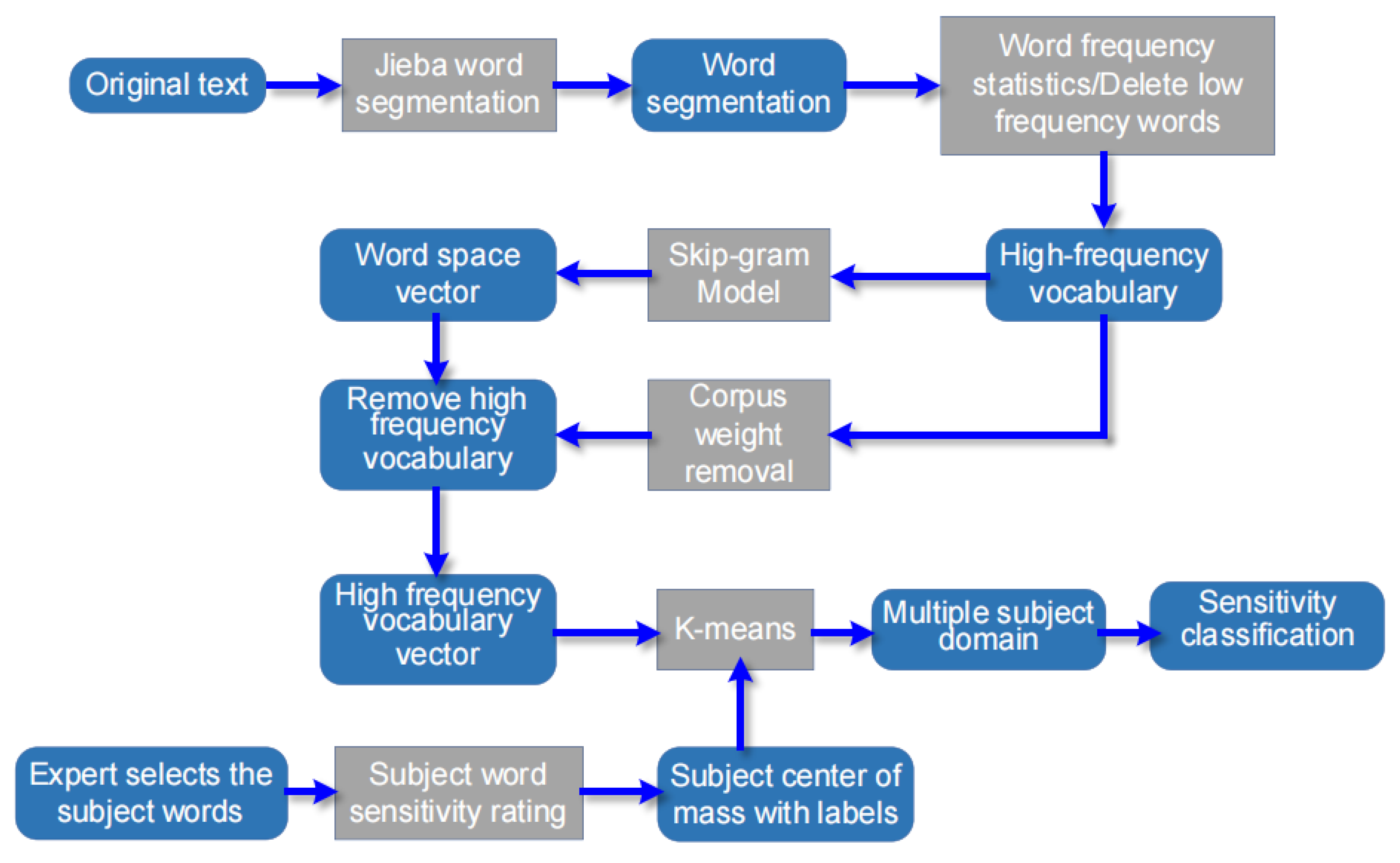
Figure 1 shows the overall architecture of the data security classification and the related method. The proposed method utilizes Jieba segmentation (Jieba is a widely-used Chinese text segmentation tool, known for its efficiency and support for various segmentation modes in natural language processing applications) to process raw text, generating a high-frequency word corpus containing both semantic and frequency information, thereby enhancing the efficiency and generalization ability of the model. Subsequently, the skip-gram model processes the high-frequency corpus, creating a word vector space. Through deduplication, vector representations of high-frequency words are obtained, serving as the training set for the K-means clustering algorithm. To improve the accuracy of sensitivity level classification, industry-expert-selected theme words are employed as the initial centroids for the K-means clustering, achieving a precise classification of the sensitivity levels in the text.

The method takes the original text as input and generates a word segmentation corpus through Jieba word segmentation processing [7]. The word segmentation corpus contains all the semantic information and word frequency information in the original text. The low-frequency words in the word segmentation corpus are identified through frequency statistics [8]. Subsequently, all instances of such words are removed from the corpus. The obtained high-frequency word database can improve the generalization ability of subsequent training models. The skip-gram model [9] further processes the high-frequency corpus, which generates the word vector space of the corpus. The model additionally incorporates the underrepresented high-frequency vocabulary into the corpus. The vector representation of all high-frequency word data obtained serves as the training set for the subsequent clustering algorithm.

k points are usually randomly selected as the initial centroid in K-means clustering [10]. This selection method is dependent on the initial value of the centroid [11], and inappropriate centroids may cause the algorithm to fall into a local optimal solution. Even descriptive texts of the same sensitivity level may have semantic differences. For example, “customer name”, “customer ID card number”, and “net investment asset value” are all text of the same sensitivity level. However, there is a significant semantic difference between “net investment asset value” and the other two fields, and the clustering algorithm is likely to divide them into different clusters. The initial centroid selection to address this problem requires industry professionals who can precisely choose multiple keywords. Each keyword is assigned a sensitivity level, such as assigning the keywords “customer” and “asset” to the same level of sensitivity. These keywords will be utilized for clustering to generate multiple topic domains. The sensitivity level of the fields contained in each subject field is the same as that of the subject word, which can precisely divide the sensitivity level.

The keywords selected by experts need to be entered before clustering to improve the accuracy of sensitivity classification. The sensitivity level of keywords is scored, and a labeled subject centroid is obtained as the initial centroid of the K-means clustering algorithm. Finally, the K-means clustering algorithm divides the data space into multiple subject domains through iterative optimization of the training set. Each subject domain corresponds to a subject word, and the sensitivity level of all corpuses in that domain is the sensitivity level of the subject word. The sensitivity classification results of all the original texts are obtained in this way.

2.1. Hierarchical Model of Sensitive Data Based on Topic Domain Division

Using parameters can better understand the sensitive-data classification model based on subject domain division. A mathematical description is given of data preprocessing and word vector acquisition. The basic rules of keyword selection and labeling are combined to further introduce the details of K-means clustering and the iterative optimization process. Finally, the mapping method of each subject domain is provided, along with the corresponding sensitivity level.

2.1.1. Parameter Definition

Original text set X is defined as follows.

$$X=\left\{X^{\left(1\right)},X^{\left(2\right)},\dots ,X^{\left(u\right)}\right\}$$

(1)

where $X^{\left(i\right)}$ represents the ith original text in original text set X and u represents the amount of text (the number of all data fields).

The definition of word segmentation $X_s^{\left(i\right)}$ is as follows after performing word segmentation on the ith original text.

$$X_s^{\left(i\right)}=\left\{x_1^{\left(i\right)},x_2^{\left(i\right)},\dots ,x_{t^{\left(i\right)}}^{\left(i\right)}\right\}$$

(2)

where $x_j^{\left(i\right)}$ represents the jth word in the word segmentation corpus $X_s^{\left(i\right)}$ and $t^{\left(i\right)}$ represents the number of words contained in the word segmentation corpus $X_s^{\left(i\right)}$.

According to the corpus dictionary D derived from the word segmentation corpus,

$$D=\left\{x_1,x_2,\dots ,x_r\right\}$$

(3)

where $x_i$ represents the ith word in the dictionary D and r represents the number of words contained in the dictionary D.

The word segmentation corpus is used for word frequency statistics, and the word frequency table F is defined as

$$F=\left\{f_1,f_2,\dots ,f_r\right\}$$

(4)

$$f_i=\frac{n_{x_i}}{N}$$

(5)

where $f_i$ represents the frequency of word $x_i$ in the word segmentation corpus; $n_{x_i}$ represents the number of occurrences of word $x_i$ in the same corpus; and N represents the total number of occurrences of all words from the dictionary D in this corpus.

The high-frequency word corpus $X_f$ is as follows after deleting low-frequency words in the word segmentation corpus.

$$X_f=\left\{X_f^{\left(1\right)},X_f^{\left(2\right)},\dots ,X_f^{\left(u_f\right)}\right\}$$

(6)

where $X_f^{\left(i\right)}$ represents the ith corpus in the high-frequency word corpus $X_f$ and $u_f$ represents the number of corpus contained in the high-frequency word corpus $X_f$.

The word vector space V is as follows through high-frequency word database training.

$$V={\left\{v_1,v_2,\dots ,v_c\right\}}^{\top }\in {\mathbb{R}}^{c\times n}$$

(7)

where $v_i$ represents the ith word’s corresponding word vector $x_i$; c represents the number of words in the word vector space V; and n represents the dimension of the word vector in the word vector space.

Deleting the corpuses that appear repeatedly in the high-frequency word database can map the words in the corpus using the word vector space V. The vector representation of the obtained high-frequency word material $V_f$ is as follows.

$$V_f={\left\{V_f^{\left(1\right)},V_f^{\left(2\right)},\dots ,V_f^{\left(m\right)}\right\}}^{\top }\in {\mathbb{R}}^{m\times n}$$

(8)

where $V_f^{\left(i\right)}$ represents the vector representation of the ith high-frequency word material and m represents the number of vectors contained within the vector $V_f$ of the high-frequency lexical material.

2.1.2. Data Preprocessing and Word Vector Acquisition

The original text set is unprocessed descriptive text. A series of preprocessing steps can produce a more accurate word vector to remove interfering factors, such as low-frequency words and stop words.

Regular expressions can be used to remove non-Chinese characters (e.g., letters, numbers, and symbols) contained in the original text set X. Jieba is utilized to perform word segmentation processing on the original text set X [7] after cleaning the text. Each original text $X^{\left(i\right)}$ is cut into a collection of multiple words or phrases $X_s^{\left(i\right)}=\left\{x_1^{\left(i\right)},x_2^{\left(i\right)},\dots ,x_{t^{\left(i\right)}}^{\left(i\right)}\right\}$, which is called the word segmentation corpus. The collection of all word segmentation corpuses is called the word segmentation corpus.

The word frequency statistics technique is used to count each word in the word segmentation corpus $X_S$. The word frequency is calculated by Equations (3)–(5) to obtain the corpus dictionary D and corpus word frequency table F of the word segmentation corpus. The word frequency in the text conforms to a long-tail pattern [12], where a small number of words occur frequently when the majority of words have low frequencies. The word vectors of these low-frequency words are difficult to train, which affects their quality and accuracy. Therefore, it is necessary to delete low-frequency words [13] to reduce the impact on the generalization ability of word vectors.

The segmentation corpus is refined by removing low-frequency words to obtain the corpus of high-frequency words. Any piece of data conforms to Equation (9).

$$f_j\ge Threshold,\forall x_j^{\left(i\right)}\in X_f^{\left(i\right)}$$

(9)

where $x_j^{\left(i\right)}$ represents any word in the corpus $X_f^{\left(i\right)}$; $f_j$ represents the frequency of the word $x_j^{\left(i\right)}$ in the corpus word frequency table F; Threshold represents the criterion for categorizing words as low-frequency, and any word with a frequency lower than this value is considered low-frequency.

The skip-gram model is utilized for training the acquired high-frequency word database $X_f$ to derive the word vector space V of the corpus.

The high-frequency vocabulary database $X_f$ is de-emphasized to obtain the high-frequency corpus through this process, which can simplify the subsequent K-means clustering model. The vector representation of the high-frequency lexical material is obtained through the word vector space V and Equation (10).

$$V_f^{\left(i\right)}=\frac{{\sum }_j^{t^{\left(i\right)}}{v}_j^{\left(i\right)}}{t^{\left(i\right)}}$$

(10)

where $V_f^{\left(i\right)}$ represents the vector of the ith high-frequency corpus after duplication; $v_j^{\left(i\right)}$ represents the word vector of the jth word in this corpus; and $t^{\left(i\right)}$ represents the number of words contained in this corpus.

2.1.3. Selection and Annotation of Subject Words

The introduction of expert-selected keywords as initial centroids is essential to enhance the accuracy of classification results before conducting K-means clustering on the vector representation $V_f$ of high-frequency word materials. Meanwhile, the keywords are categorized based on their sensitivity level following industry standards. The selection of keywords should follow the following principles.

Relevance: The keywords should be related to the content of the description text and reflect the main content and key information of the text.

Representativeness: Keywords should represent the overall content of the text.

Inclusiveness: Keywords should contain important information and cover as many aspects of the text as possible.

Validity: Keywords should have a degree of distinction; there should be obvious differences in keywords between different topics.

The selected keyword set is expressed as T.

$$T=\left\{x_1,x_2,\dots ,x_k\right\}$$

(11)

where $x_i$ represents the ith word the keyword set T and k represents the number of keywords contained within T.

The sensitivity level of keywords must be marked according to clearly defined standards to avoid the effects of subjectivity and inconsistency. The sensitivity level ratio for keyword labeling should align with that of the descriptive text to avoid excessive preference or neglect of certain topics by subsequent models.

The keyword sensitivity level is expressed as $L_T$ after the labeling.

$$L_T=\left\{l_1,l_2,\dots ,l_k\right\}$$

(12)

where $l_i$ represents the sensitivity level of the ith word $x_i$ in the keyword set T.

2.2. K-Means Clustering

Data preparation for the K-means clustering has been completed after obtaining the vector representation $V_f$ of the high-frequency word material and the subject word’s sensitive level representation $L_T$. The k-value and initial centroid in the cluster have been determined by the keywords. The clustering training of data only needs to choose the appropriate distance measurement method.

2.2.1. Choice of Distance Measurement Method

Commonly used distance measurement methods include Euclidean distance [14,15], Manhattan distance [15,16], cosine similarity [17,18], etc. The following factors need to be considered when a distance measurement method is selected in K-means clustering [19,20].

Data type. The distance measurement method should apply to the data type. For example, Euclidean distance, Manhattan distance, and cosine similarity can be used separately for continuous numerical data, binary or discrete data, and text data.

Data characteristics. The distance measurement method should capture the data characteristics. For instance, Euclidean distance is suitable for data considering numerical differences in various dimensions, while cosine similarity is suitable for vector data considering the direction and angle relationship.

Data distribution. The distance measurement method should be capable of processing data under different data distributions. Some distance measurement methods are sensitive to outlier values, while others can better cope with data with skewed or long-tail distributions.

Algorithm performance. The algorithm performance can be influenced by the computational complexity of the distance measurement method. The time-consuming nature of certain distance measurement methods necessitates careful consideration of algorithm efficiency, particularly when dealing with large-scale data sets.

The cosine similarity measure is particularly suitable for text-like data, as it disregards the text length and instead focuses on capturing the directional similarity between vectors, rather than specific numerical differences. Therefore, cosine similarity is selected as the distance measurement method for K-means clustering, which is obtained from Equation (13).

$$S_{cosine}\left(v_1,v_2\right)=\frac{v_1·v_2}{\parallel v_1\parallel ·\parallel v_2\parallel }$$

(13)

where $v_1$ and $v_2$ represent two nonzero vectors and $\parallel ·\parallel$ represents the modulus calculation of the vector.

2.2.2. Optimization Process of Clustering

The selected keyword set is mapped from the word vector space V to the initial centroid set, which is expressed as C.

$$C=\left\{c_1,c_2,\dots ,c_k\right\}$$

(14)

where $c_i$ represents the ith centroid in centroid set C and k represents the number of centroids in the K-means cluster.

Clustering can directly enter the iterative optimization process since the initial centroid has been determined by the subject word. Each iteration consists of two steps: assigning data points and updating the cluster center point.

Assign data points. Cosine similarity to the center $c_j$ of each cluster is calculated according to Equation (13) for vector representation $V_f^{\left(i\right)}$ of each high-frequency corpus. The cluster center to which the vector representation belongs in this iteration is selected according to Equation (15).

$${argmax}_{c_j}{S}_{cosine}\left(V_f^{\left(i\right)},c_j\right),\forall j\in \left[k\right]$$

(15)

Update the cluster center point. The value of each cluster center needs to be recalculated according to Equation (16) after all vector representations are assigned to the corresponding cluster centers. Then, the updated cluster center value is used for the next iteration.

$$c_j^{\left(p+1\right)}=\frac{{\sum }_i^{{num}_j^{\left(p\right)}}{V}_f^{\left(i\right)}}{{num}_j^{\left(p\right)}}$$

(16)

where $c_j^{\left(p+1\right)}$ represents the cluster center j obtained from the p + 1 round in the pth iteration; $V_f^{\left(i\right)}$ represents any vector representation assigned to the cluster center j in the pth iteration; and ${num}_j^{\left(p\right)}$ represents the number of vector representations assigned to the cluster center j in the pth iteration.

The two steps are repeated until the clustering center point no longer changes, or the iteration is stopped when the maximum number of iterations is reached.

2.2.3. Sensitivity Level Mapping of the Topic Domain

Each vector representation is assigned to a domain in the cluster center after completing the iterative optimization of clustering. This domain corresponds to a keyword in the keyword set T, which is called the subject domain [21]. Any cluster label of vector representation $V_f^{\left(i\right)}$ belongs to interval $[1,k]$, where k denotes the number of cluster centers. The label is mapped using the subject term sensitivity level so that the sensitivity level classification of the vector representation can be displayed. The mapping method is shown in Equation (17).

$$i\to l_i,\forall i\in \left[1,k\right],l_i\in L_T$$

(17)

where i represents the cluster label and $l_i$ represents the keyword sensitivity level label.

Each original text has been trained to obtain a sensitivity level division, and the cluster center set C and keyword sensitivity level $L_T$ after the iteration are saved. Thus, the sensitivity level can be judged according to Equations (15) and (17) for any original text.

2.3. Sensitive Data Classification Algorithm

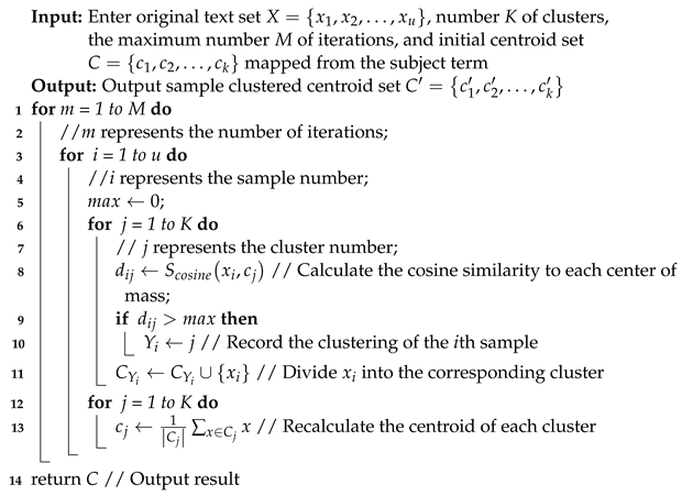
The pseudo-code of the sensitive data classification model based on subject domain division is presented below after being derived through the mathematical deduction of the equation. For each instance, its cosine similarity to each centroid is first calculated to divide it into corresponding clusters. Then, based on the samples in each cluster, the centroid of the cluster is recalculated. Iterate in this order until the center of mass no longer changes or the maximum number of iterations is reached. See Algorithm 1.    

Algorithm 1: Sensitive data classification algorithm based on subject domain division.

3. Results and Discussion

The model’s performance was assessed, and its deployability was validated by evaluating the impact of weak semantic information in sensitive data fields on sensitivity level judgments, as well as its ability to accurately judge real-world business data.

The following indicators were used in this experiment to evaluate the accuracy of the clustering model’s sensitivity level division of the training set after fitting. The confusion matrix [22] and the squared error [23] were two commonly used evaluation indicators in multi-classification problems. Additionally, the average distance within clusters [24] and the average distance between clusters [25,26] were two commonly used indicators for evaluating the effectiveness of clustering algorithms. About 143 frequently used descriptive texts were selected to verify the usability of the algorithm in the face of real business data. The model was used to judge the sensitivity level and calculate the prediction accuracy. In addition, the text with prediction errors was analyzed in detail to find the bias of the model. Then, the model’s prediction results could be promptly rectified in practical scenarios.

3.1. Data Set Introduction and Preprocessing

The data set used in this work was a descriptive text library of a financial institution in China. The training set comprised 334,065 text fields in the entire business scenario. Test set 1 encompassed 57 text fields about individual customers in the trust business. Test set 2 encompassed 88 text fields related to institutional customers in the trust business. The sensitivity levels of the fields in this data set were categorized into three tiers: low-sensitivity fields, mid-sensitivity fields, and high-sensitivity fields, according to Chinese laws, regulations, and financial institution policies. For example, the account number and account name are low-sensitivity fields; the residence, ID number, and postal code are medium-sensitivity fields; and passwords are high-sensitivity fields.

The following preprocessing tasks were required to make data meet the input requirements of the K-means clustering algorithm after obtaining the information of the data set:

i

Use regular expressions to remove non-Chinese characters such as letters, symbols, and numbers from the original text.

ii

Perform Jieba segmentation on 334,065 texts to obtain 334,065 word segmentation materials.

iii

Perform word frequency statistics on the word segmentation corpus. Delete the text containing words with a word frequency of less than 100 to obtain 263,796 high-frequency word materials.

iv

Use the skip-gram model to train 263,796 high-frequency word materials to obtain a 10-dimensional word vector of 1414 words.

v

Carry out weight removal of 263,796 high-frequency word materials to obtain 21,346 high-frequency word materials.

vi

Select 184 subject words according to the experience of experts, and mark the corresponding sensitivity level.

Table 1. Data set display.

Data Name	Data Total	Number of Low-Sensitivity Fields	Number of Mid-Sensitivity Fields	Number of High-Sensitivity Fields
Training set	21,346	18,839	2481	26
Test set 1	56	42	14	1
Test set 2	87	71	16	1
Subject term	184	150	33	1

lists the specific quantities of data with varying sensitivity levels in different data types.

3.2. Experimental Results and Index Evaluation

This section first defines the experimental evaluation indicators in detail. The validity of the sensitive data classification model, which is based on subject domain division and its applicability in real business scenarios, has been verified through multiple indices. The verification process proves the advanced nature of the algorithm and finds out its shortcomings.

3.2.1. Experimental Evaluation Index Definition

(1) Sensitivity classification accuracy. The accuracy of sensitivity classification is defined as follows.

$$Accuracy=\frac{N_c}{N_{all}}$$

(18)

where $N_{all}$ represents the total number of texts to be graded and $N_c$ represents the number of texts to be graded correctly.

(2) Sum squared error. The formula for the sum squared error is defined as follows.

$$SSE=\sum _{c_j\in C}\sum _{V_f^{\left(i\right)}\in c_j}{\left(1-S_{cosine}\left(V_f^{\left(i\right)},c_j\right)\right)}^2$$

(19)

where $c_j$ represents the jth centroid in centroid set C and $V_f^{\left(i\right)}$ represents the vector representation of the corpus belonging to centroid $c_j$.

(3) Confusion matrix. Any value ${CM}_{ij}$ in the confusion matrix is defined as the number of texts where the real label belongs to the ith category and the predicted label belongs to the jth category.

(4) Intra-cluster average distance. The formula for the intra-cluster average distance is defined as follows.

$$Intr{a}_{{CAD}_b}=\frac{{\sum }_{V_f^{\left(j\right)}\in c_b}{\sum }_{V_f^{\left(i\right)}\in c_b}\left(1-S_{cosine}\left(V_f^{\left(i\right)},V_f^{\left(j\right)}\right)\right)}{w_b\left(w_b-1\right)}$$

(20)

where $Intr{a}_{{CAD}_b}$ represents the intra-cluster average distance of centroid $c_b$; $V_f^{\left(i\right)}$ and $V_f^{\left(j\right)}$ represent the vector representation of the corpus belonging to centroid v; and $w_b$ represents the number of vector representations of the corpus belonging to centroid $c_b$.

(5) Inter-cluster average distance. The formula for the inter-cluster average distance is defined as follows.

$$Inte{r}_{CAD}=\frac{{\sum }_{c_i\in C}{\sum }_{c_j\in C}\left(1-S_{cosine}\left(c_i,c_j\right)\right)}{k\left(k-1\right)}$$

(21)

where $c_i$ and $c_j$ represent the centroids belonging to centroid set C and k represents the number of centroids in the cluster.

3.2.2. Validity Verification Experiment of Sensitivity Classification

This experiment will fit a sensitive data classification model based on subject domain division on the training set. Changes in key indicators are shown, such as the accuracy and sum squared error during the fitting process. The final prediction accuracy and confusion matrix of the model on the training set are provided to ensure the efficacy of sensitive data classification after completing the model training. The intra-cluster average distance and inter-cluster average distance are compared in detail to further validate the scientific validity of the expert-selected keywords after fitting the model.

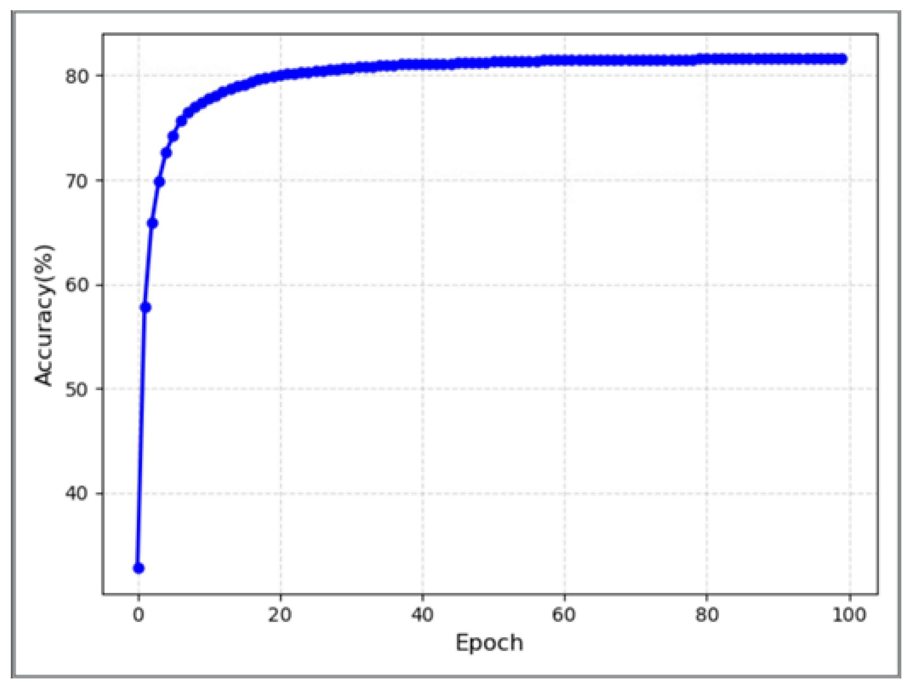
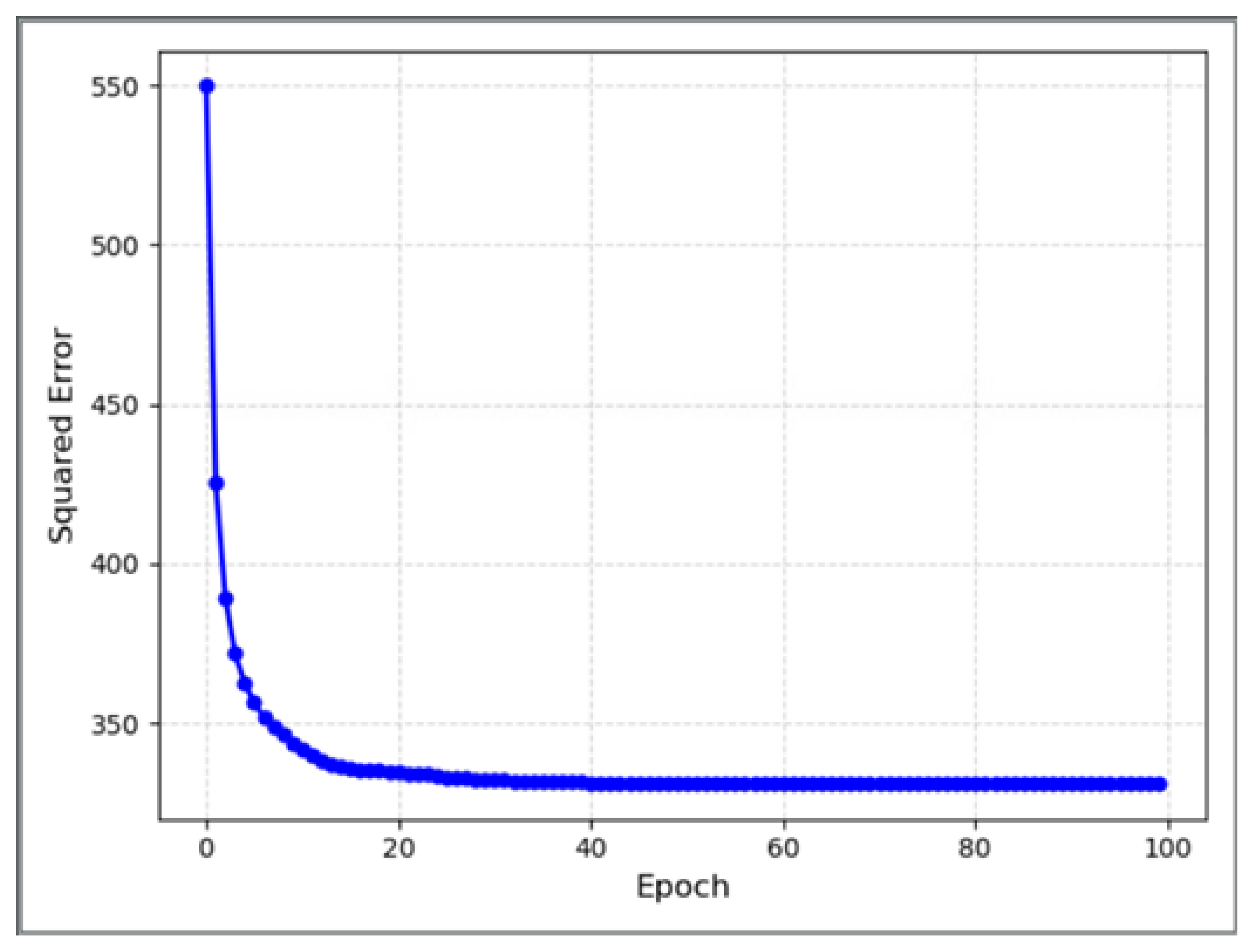
Figure 2 and Figure 3 show the accuracy and sum squared error of each optimization iteration of this model during the fitting process, respectively. The horizontal coordinates all represent the number of iterations, and its maximum number is 100. The vertical coordinates represent the accuracy and sum squared error, respectively.

As the number of model iterations increases, the accuracy rate continues to rise, while the sum squared errors continue to decrease from these two figures. The change rate of the two indicators is identical, which proves the model makes progress in the learning task and enhances the performance in the prediction task. The two curves exhibit a consistent pattern without any noticeable fluctuations or shocks, indicating the model’s relative stability during the training process. The indicators both converge to the optimal value, an the accuracy of approximately 81.59% and a sum squared error of around 330. Therefore, the efficacy of this model in the classification of sensitive data has been demonstrated.

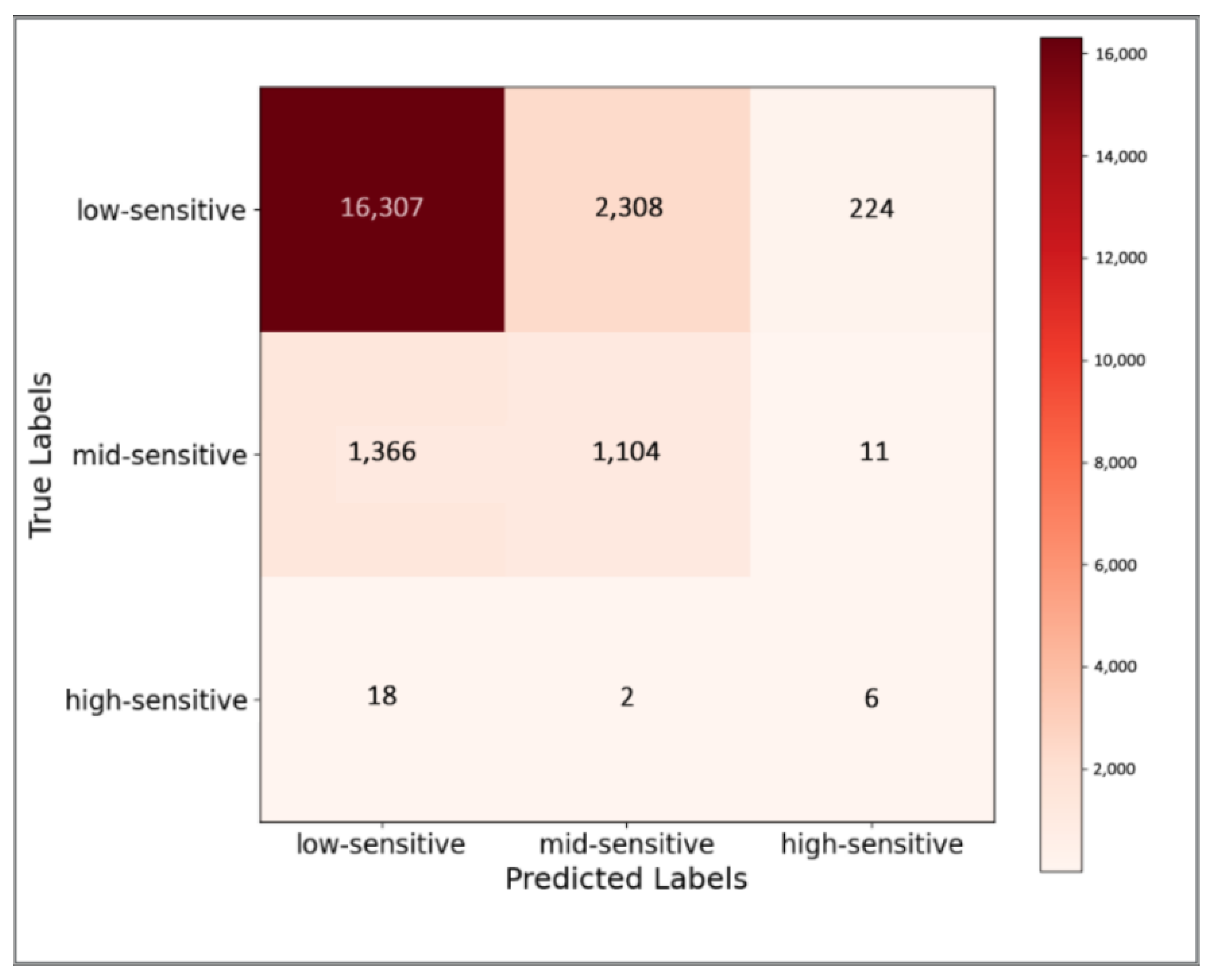
Figure 4 shows the confusion matrix (CM) of the model’s final prediction on the training set. The rows of the matrix represent the real labels of the text, while the columns represent the model’s predictive labels. In addition, the number of texts belonging to this category is marked in each cell of the matrix.

The model exhibits a high accuracy in predicting the overall three sensitive levels of data. However, it may have a certain impact on predictions for other levels due to the training set’s text being biased toward the low-sensitivite level. Unbiased prediction based on biased data is the improvement direction of the model.

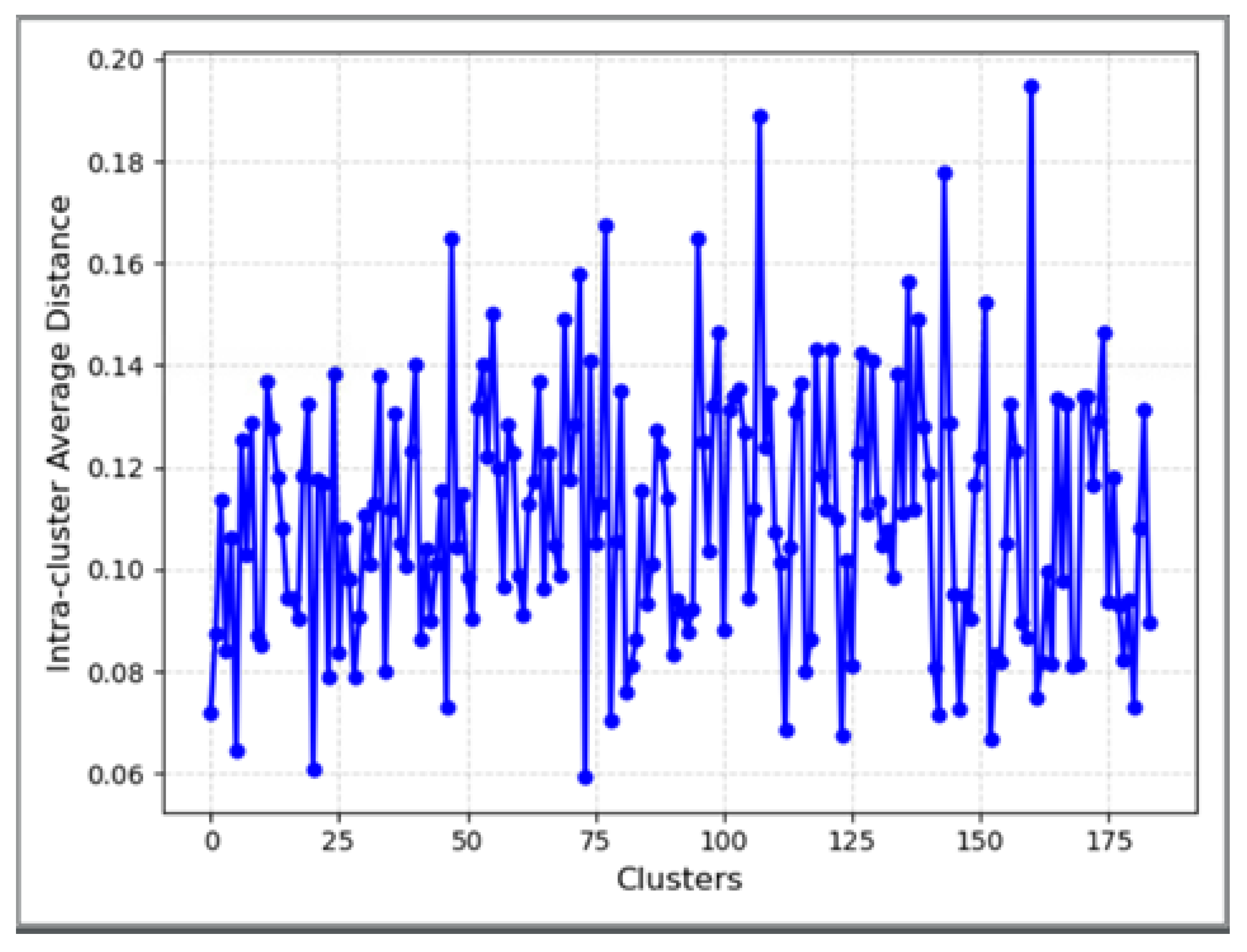
Figure 5 shows the intra-cluster average distance of each category after training the model. The x-axis is 184 clustering centers, and the y-axis is the intra-cluster average distance.

The intra-cluster average distance of each category is within interval $[0.06,0.20]$ in Figure 5, proving that the clustering tightness within each category is higher [24]. The greater similarity in similar examples further substantiates the experts’ scientific selection of keywords.

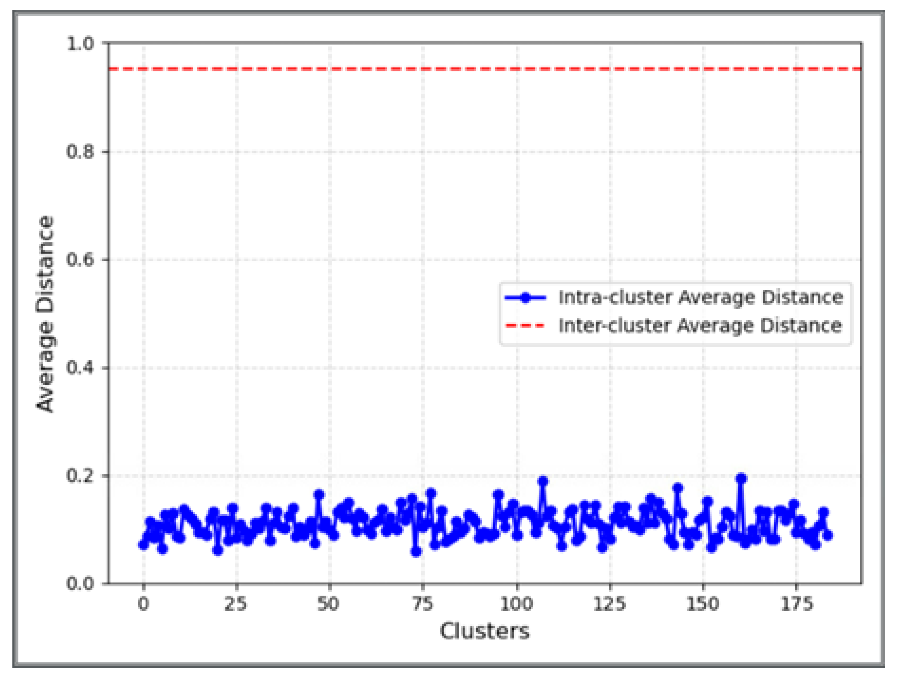
Figure 6 compares the inter-cluster average distance with the intra-cluster average distance, which intuitively shows the clustering separation degree. The x- and y-axes, red dotted line, and blue line represent 184 cluster centers, the average distance, the inter-cluster average distance, and the intra-cluster average distance, respectively.

The inter-cluster average distance is about 0.95, which is much higher than the maximum value of the intra-cluster average distance. The differences between samples are large in different clusters, with high similarities between samples in the same cluster. The model performs well in classifying similar samples into the same clusters, and the boundaries between different clusters are relatively clear. The clustering results in this case are satisfactory, which validates the experts’ scientific selection of keywords.

3.2.3. Usability Verification Experiments for Real Business Scenarios

This experiment validated the algorithm’s utility with real-world business data after demonstrating the efficacy of this model in sensitivity level classification. The evaluation metrics for the experiment included the sensitivity classification accuracy and confusion matrix of the model on both test sets.

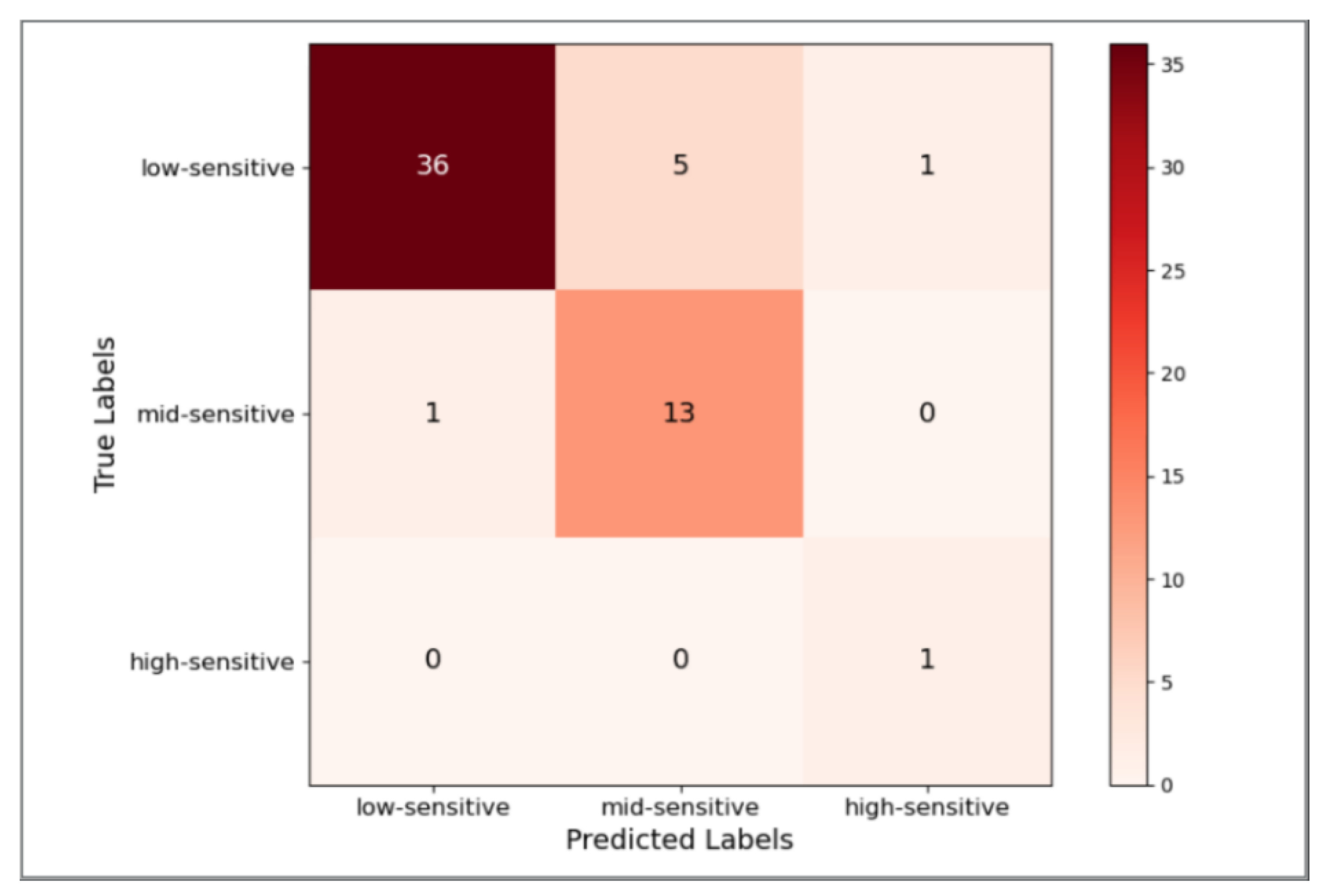
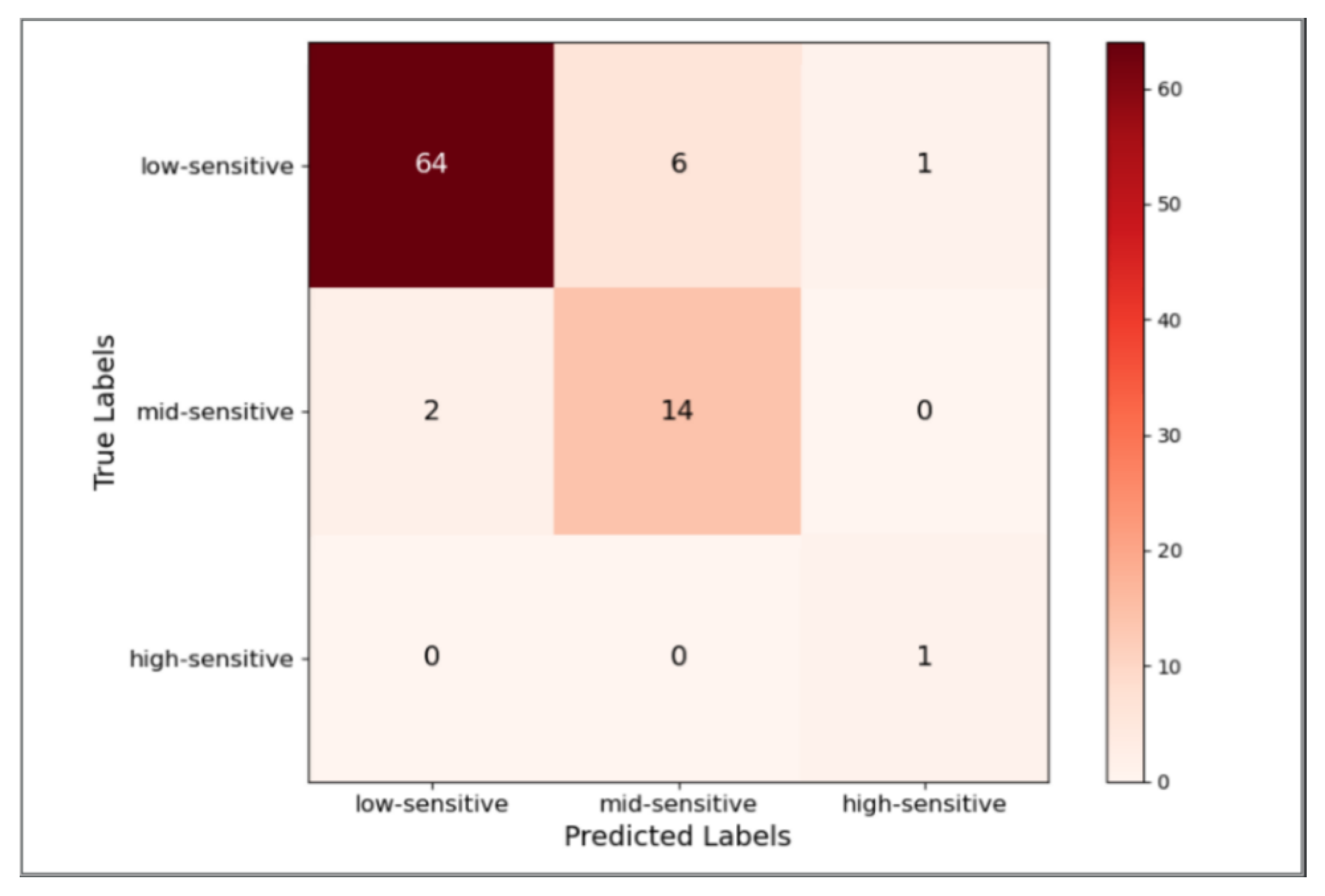
Figure 7 and Figure 8 show the confusion matrix of this model after the sensitivity level prediction on test sets 1 and 2, respectively.

The calculation accuracy of the sensitivity level division of the model on test sets 1 and 2 is 87.72 and 89.77%, respectively, proving the usability of the model on real business data. This work analyzes the text incorrectly predicted in two test sets to further identify the direction of model improvement. Most of them are relatively infrequent words or unknown words that do not appear in the training set [27]. When faced with such words, the semantic information that the model can extract is weak, which leads to incorrect predictions. Therefore, it is imperative to incorporate text containing such words for the incremental training of our model [28] to rectify the semantic information of words. This approach can enhance the algorithm performance and continuously optimize the model in real-world business scenarios.

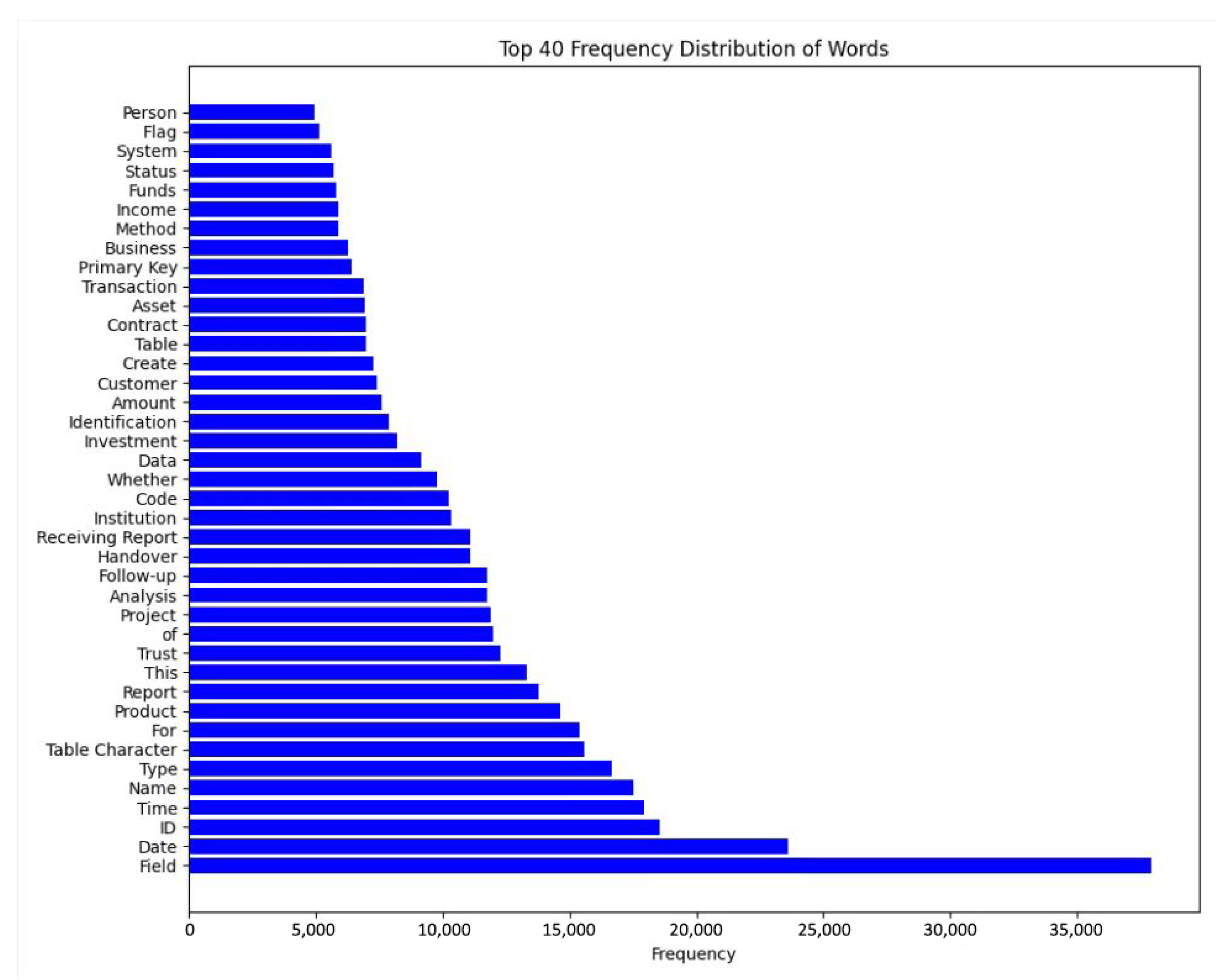
In order to display the distribution of word frequency more intuitively, Figure 9 shows the 40 word segmentation results with the highest frequency.

The aforementioned experimental results demonstrate that the proposed model achieves an accuracy exceeding 80% in sensitivity level classification across all three data sets, which can segregate sensitive data. In addition, its performance on the test set is better than that on the training set, and the model performance can be optimized through incremental training. Therefore, the model can meet the requirements for sensitive data partitioning in real business scenarios and can be well applied to data security classification and grading work in various fields.

Our method relies heavily on experts’ selection of subject words. Therefore, how to reduce the bias caused by experts’ subjective reasons is our future research direction.

4. Conclusions

The improper partitioning of sensitive data reduces the security of highly sensitive data as well as the availability of low-sensitivity data. Therefore, the security classification and grading of sensitive data needed to be addressed. Relevant research showed a lack of effective sensitivity level classification methods for data with weak semantic information. Moreover, it was difficult to propose a universal model due to the different rules for dividing data sensitivity levels in various fields.

This work proposed a sensitive data classification model based on topic domain partitioning. A series of evaluation indices were used to experimentally demonstrate the effectiveness of the algorithm in sensitivity level partitioning and its usability in real business scenarios. The contributions of this work are as follows:

a

The issue of classifying text with weak semantic information at a sensitive level has been addressed, with the practicality and applicability of the proposed method significantly enhanced. This advancement has facilitated the implementation of sensitive data classification and grading efforts, which established a solid foundation for ensuring data security protection.

b

The limitations of data on the extensibility of the model were eliminated from different fields. The data of different industries and fields were only related to keywords by introducing the experts’ selection of keywords; therefore, the model could be applied to various fields.

c

Optimization strategies were proposed for the model in real-world business scenarios to continuously enhance its performance in practical applications and dynamically monitor changes in sensitive data.

References

- Abraham, R.; Schneider, J.; Vom Brocke, J. Data governance: A conceptual framework, structured review, and research agenda. Int. J. Inf. Manag. 2019, 49, 424–438. [Google Scholar] [CrossRef]
- Karkošková, S. Data governance model to enhance data quality in financial institutions. Inf. Syst. Manag. 2023, 40, 90–110. [Google Scholar] [CrossRef]
- Huang, J.; Li, Z.; Xiao, X.; Wu, Z.; Lu, K.; Zhang, X.; Jiang, G. SUPOR: Precise and scalable sensitive user input detection for android apps. In Proceedings of the 24th USENIX Security Symposium (USENIX Security 15), Washington, DC, USA, 12–14 August 2015; pp. 977–992. [Google Scholar]
- Nan, Y.; Yang, M.; Yang, Z.; Zhou, S.; Gu, G.; Wang, X. Uipicker: User-input privacy identification in mobile applications. In Proceedings of the 24th USENIX Security Symposium (USENIX Security 15), Washington, DC, USA, 12–14 August 2015; pp. 993–1008. [Google Scholar]
- Yang, Z.; Liang, Z. Automated Identification of Sensitive Data via Flexible User Requirements. In Security and Privacy in Communication Networks, Proceedings of the 14th International Conference, SecureComm 2018, Singapore, 8–10 August 2018; Proceedings, Part I; Springer International Publishing: Cham, Switzerland, 2018; pp. 151–171. [Google Scholar]
- Gitanjali, K.L. A novel approach of sensitive data classification using convolution neural network and logistic regression. Int. J. Innov. Technol. Explor. Eng. 2019, 8, 2883–2886. [Google Scholar]
- Zhang, X.; Wu, P.; Cai, J.; Wang, K. A contrastive study of Chinese text segmentation tools in marketing notification texts. J. Phys. Conf. Ser. 2019, 2, 022010. [Google Scholar] [CrossRef]
- Baron, A.; Rayson, P.; Archer, D. Word frequency and key word statistics in corpus linguistics. Anglistik 2009, 20, 41–67. [Google Scholar]
- Guthrie, D.; Allison, B.; Liu, W.; Guthrie, L.; Wilks, Y. A closer look at skip-gram modelling. In Proceedings of the LREC, Genoa, Italy, 22–28 May 2006; Volume 6, pp. 1222–1225. [Google Scholar]
- Likas, A.; Vlassis, N.; Verbeek, J.J. The global k-means clustering algorithm. Pattern Recognit. 2003, 36, 451–461. [Google Scholar] [CrossRef]
- Mahmud, M.S.; Rahman, M.M.; Akhtar, M.N. Improvement of K-means clustering algorithm with better initial centroids based on weighted average. In Proceedings of the 2012 7th International Conference on Electrical and Computer Engineering, Dhaka, Bangladesh, 20–22 December 2012; pp. 647–650. [Google Scholar]
- Nadeem, M.I.; Ahmed, K.; Li, D.; Zheng, Z.; Naheed, H.; Muaad, A.Y.; Alqarafi, A.; Abdel Hameed, H. SHO-CNN: A Metaheuristic Optimization of a Convolutional Neural Network for Multi-Label News Classification. Electronics 2022, 12, 113. [Google Scholar] [CrossRef]
- Li, F.; Wang, X. Improving word embeddings for low frequency words by pseudo contexts. In Proceedings of the Chinese Computational Linguistics and Natural Language Processing Based on Naturally Annotated Big Data: 16th China National Conference, CCL 2017, and 5th International Symposium, NLP-NABD 2017, Nanjing, China, 13–15 October 2017; Proceedings 16. Springer International Publishing: Cham, Switzerland, 2017; pp. 37–47. [Google Scholar]
- Danielsson, P.E. Euclidean distance mapping. Comput. Graph. Image Process. 1980, 14, 227–248. [Google Scholar] [CrossRef]
- Sinwar, D.; Kaushik, R. Study of Euclidean and Manhattan distance metrics using simple k-means clustering. Int. J. Res. Appl. Sci. Eng. Technol. 2014, 2, 270–274. [Google Scholar]
- Chiu, W.Y.; Yen, G.G.; Juan, T.K. Minimum manhattan distance approach to multiple criteria decision making in multiobjective optimization problems. IEEE Trans. Evol. Comput. 2016, 20, 972–985. [Google Scholar] [CrossRef]
- Rahutomo, F.; Kitasuka, T.; Aritsugi, M. Semantic cosine similarity. In Proceedings of the 7th International Student Conference on Advanced Science and Technology ICAST, Seoul, Republic of Korea, 29–30 October 2012; Volume 4, p. 1. [Google Scholar]
- Muflikhah, L.; Baharudin, B. Document clustering using concept space and cosine similarity measurement. In Proceedings of the 2009 International Conference on Computer Technology and Development, Kota Kinabalu, Malaysia, 13–15 November 2009; Volume 1, pp. 58–62. [Google Scholar]
- Singh, A.; Yadav, A.; Rana, A. K-means with Three different Distance Metrics. Int. J. Comput. Appl. 2013, 67, 14–17. [Google Scholar] [CrossRef]
- Kapil, S.; Chawla, M. Performance evaluation of K-means clustering algorithm with various distance metrics. In Proceedings of the 2016 IEEE 1st International Conference on Power Electronics, Intelligent Control and Energy Systems (ICPEICES), Delhi, India, 4–6 July 2016; pp. 1–4. [Google Scholar]
- Yi, J.; Nasukawa, T.; Bunescu, R.; Niblack, W. Sentiment analyzer: Extracting sentiments about a given topic using natural language processing techniques. In Proceedings of the Third IEEE International Conference on Data Mining, Melbourne, FL, USA, 22–22 November 2003; pp. 427–434. [Google Scholar]
- Caelen, O. A Bayesian interpretation of the confusion matrix. Ann. Math. Artif. Intell. 2017, 81, 429–450. [Google Scholar] [CrossRef]
- Thinsungnoena, T.; Kaoungkub, N.; Durongdumronchaib, P.; Kerdprasopb, K.; Kerdprasopb, N. The clustering validity with silhouette and sum of squared errors. Learning 2015, 3, 44–51. [Google Scholar]
- Chiang, M.M.T.; Mirkin, B. Intelligent choice of the number of clusters in k-means clustering: An experimental study with different cluster spreads. J. Classif. 2010, 27, 3–40. [Google Scholar] [CrossRef]
- Shi, C.; Wei, B.; Wei, S.; Wang, W.; Liu, H.; Liu, J. A quantitative discriminant method of elbow point for the optimal number of clusters in clustering algorithm. EURASIP J. Wirel. Commun. Netw. 2021, 2021, 31. [Google Scholar] [CrossRef]
- Dinh, D.T.; Fujinami, T.; Huynh, V.N. Estimating the optimal number of clusters in categorical data clustering by silhouette coefficient. In Knowledge and Systems Sciences, Proceedings of the 20th International Symposium, KSS 2019, Da Nang, Vietnam, 29 November–1 December 2019; Proceedings 20; Springer: Singapore, 2019; pp. 1–17. [Google Scholar]
- Wei, D.; Liu, Z.; Xu, D.; Ma, K.; Tao, L.; Xie, Z.; Pan, S. Word segmentation of Chinese texts in the geoscience domain using the BERT model. ESS Open Arch. 2022. [Google Scholar] [CrossRef]
- You, C.; Xiang, J.; Su, K.; Zhang, X.; Dong, S.; Onofrey, J.; Staib, L.; Duncan, J.S. Incremental learning meets transfer learning: Application to multi-site prostate mri segmentation. In Distributed, Collaborative, and Federated Learning, and Affordable AI and Healthcare for Resource Diverse Global Health, Proceedings of the Third MICCAI Workshop, DeCaF 2022, and Second MICCAI Workshop, FAIR 2022, Held in Conjunction with MICCAI 2022, Singapore, 18 and 22 September 2022; Proceedings; Springer Nature: Cham, Switzerland, 2022; pp. 3–16. [Google Scholar]
Disclaimer/Publisher’s Note: The statements, opinions and data contained in all publications are solely those of the individual author(s) and contributor(s) and not of MDPI and/or the editor(s). MDPI and/or the editor(s) disclaim responsibility for any injury to people or property resulting from any ideas, methods, instructions or products referred to in the content. |
© 2024 by the authors. Licensee MDPI, Basel, Switzerland. This article is an open access article distributed under the terms and conditions of the Creative Commons Attribution (CC BY) license (https://creativecommons.org/licenses/by/4.0/).