Abstract
With the advent of the “Internet of Things” (IoT), insurers are increasingly leveraging remote sensor technology in the development of novel insurance products and risk management programs. For example, Hartford Steam Boiler’s (HSB) IoT freeze loss program uses IoT temperature sensors to monitor indoor temperatures in locations at high risk of water-pipe burst (freeze loss) with the goal of reducing insurances losses via real-time monitoring of the temperature data streams. In the event these monitoring systems detect a potentially risky temperature environment, an alert is sent to the end-insured (business manager, tenant, maintenance staff, etc.), prompting them to take remedial action by raising temperatures. In the event that an alert is sent and freeze loss occurs, the firm is not liable for any damages incurred by the event. For the program to be effective, there must be a reliable method of verifying if customers took appropriate corrective action after receiving an alert. Due to the program’s scale, direct follow up via text or phone calls is not possible for every alert event. In addition, direct feedback from customers is not necessarily reliable. In this paper, we propose the use of a non-linear, auto-regressive time series model, coupled with the time series intervention analysis method known as causal impact, to directly evaluate whether or not a customer took action directly from IoT temperature streams. Our method offers several distinct advantages over other methods as it is (a) readily scalable with continued program growth, (b) entirely automated, and (c) inherently less biased than human labelers or direct customer response. We demonstrate the efficacy of our method using a sample of actual freeze alert events from the freeze loss program.
1. Introduction
With the advent of the “Internet of Things”, it has become increasingly commonplace to develop real-time alerting and monitoring systems capable of mitigating the risk of mechanical failures via human intervention. Indeed, there are several challenges posed by such systems. First, the multiple time series generated in these scenarios often exhibit non-linear/non-Gaussian temporal dependencies. Next, in order for alerting mechanisms to be effective, there is a need to develop statistical methods capable of assessing the impact of exogenous interventions (alerts) in the form of spurring prompt human intervention. Finally, because there are likely thousands of such sensors involved in these types of IoT programs, any modeling paradigm must be readily scalable. In this paper, we propose a latent autoregressive Student-t process model to accomplish all three of these goals.
Intervention analysis is a well-established time series approach. An integral component of a successful intervention analysis is the use of a suitable time series model to learn the pre-intervention time series behavior. Linear models have traditionally been employed for this purpose. These include Gaussian autoregressive moving average (ARIMA) models [1,2], Gaussian dynamic linear models (DLM) [3,4], or Bayesian structural time series (BSTS) models [5,6].
In the Bayesian framework, the pre-intervention model is used to derive the joint posterior predictive distribution of post-intervention observations. Samples from this posterior predictive distribution serve as counterfactuals to the post-intervention observations. By measuring the difference between these forecast values and the observed post-intervention data, a semi-parametric posterior estimate for the impact of the intervention is constructed. Due to its simplicity and versatility, this methodology described in [6] has been employed across a wide array of disciplines. For instance, Ref. [7] adapted the BSTS model to evaluate the impact of rebates for turf removal on water consumption across many households. In the public health context, Ref. [8] evaluated the impact of bariatric surgery (used for weight loss) on health care utilization in Germany. Another interesting example is given by [9], who used the impact framework in conjunction with a variety of climate time series to assess whether an anomalous climate change event can be credibly linked to the collapse of several Bronze age civilizations in the Mediterranean region.
For intervention impact analysis to be successful, it is critical that the underlying time series model adequately captures the pre-intervention time series dynamics. Traditional linear, Gaussian models can be inadequate for capturing the dynamics of time series that exhibit complex non-linear and/or long-term dependencies, and/or non-Gaussian behavior. As a consequence, the counterfactual forecasts may be inadequate to give a useful assessment of the impact. For example, multiple time series generated by “Internet of Things” (IoT) sensors often exhibit nonlinear temporal dependence that cannot be easily modeled by BSTS models. Successful intervention analysis of such time series requires sophisticated models of pre-intervention data such as those described in this paper.
For intervention impact analysis in multiple IoT time series, Ref. [10] proposed a Gaussian process (GP) prior regression model [11] with a covariance kernel tailored for these series as the underlying predictive model. This model is effective in that it can incorporate typical time series behavior such as seasonality and local linear trends but also non-linear time trends and dependencies between the target variable and exogenous predictors. While this model was demonstrated to be effective at capturing a wide array of time series dynamics, it does not directly incorporate information from past values of the time series. In addition, the GP prior can fail for time series that exhibit a heavy-tailed behavior.
With this in mind, we propose an extension to the latent Gaussian process time series model presented in [12] in which we replace the latent GP with that of a Student-t process (TP) [13,14] that we then use as the underlying model for a time series impact analysis using both simulated and real-world time series data from the IoT domain. In addition to going beyond the GP functional prior, our model had the added versatility in that it can accommodate arbitrary likelihoods, allowing for heavy-tailed observations to be modeled in a more robust way.
Note that because we require a model that allows for posterior sampling, mixture autoregressive models such as the one proposed in [15] are not suitable for solving our problem. In addition, the mixture autoregressive assumptions described in [15] may be unsuitable to describe the data generating process of IoT time series data.
The format of this paper is as follows: Section 2 describes the IoT temperature sensors and their associated data streams; Section 3 gives an overview of GP regression, including descriptions of existing GP regression models tailored for time series. Section 4 details the requisite background information regarding TP regression; we also introduce our autoregressive TP model. Section 5 compares the performance of our proposed model with existing methods on a time series intervention analysis problem. Section 6 summarizes our findings and discusses potential avenues for future research.
2. Background
One domain in which IoT sensor technology has been successfully deployed is the insurance context. For example, insurers have used IoT temperature sensors part of freeze loss prevention programs. The goal of these programs is to reduce insurance losses due to water-pipe burst (freeze loss) by providing temperature sensors to end users (insured property owners) to be installed in areas with a high risk of water pipe burst. In an ideal scenario, losses are prevented (or at least mitigated) by sending real-time alerts to customers to promptly take remedial action (i.e., raising temperatures to a safe level) in the event of dangerously low temperatures within the monitored space.
In this paper, we apply our methods to sensor temperature readings that are relayed in real time at a 15 min frequency. For each sensor stream, a decision rule algorithm combines information from (a) recent sensor readings and (b) outdoor temperatures from nearby weather stations to alert end users of potential imminent freeze loss. After receiving an alert, an end user is expected to take remedial action within 12 h of receiving the alert. Due to the program’s scale, it is impossible to directly verify whether a customer took corrective action. Therefore, methods must be developed that can infer customer action only from the observed post-alert sensor streams themselves. To that end, we employ the causal impact methodology proposed by [6], which uses a counter-factual forecasting model to infer whether the alert system is effective in instigating customer action for a given alert event. More details, as well as an example of an alert event, can be found in Section 5.
3. Review of Gaussian Process Regression Models
We review the basic Gaussian process (GP) regression and its extensions for analyzing time series. Section 3.1 summarizes standard GP and regression techniques. Section 3.2 reviews the current literature on using nonlinear auto-regressions with exogenous predictors (NARX) in conjunction with GP regression (GP-NARX) models. In Section 3.3, we give a detailed review of the GP-RLARX model, a robust time series regression model that uses an auto-regressive latent state whose transition functions follow a GP prior, and the observations follow a normal distribution with time-varying scale.
3.1. GP and Sparse GP Regression
Gaussian processes (GP) are a set of methods that generalize the multivariate normal to infinite dimensions. Not only do GPs have a flexible non-parametric form, GP methods are also attractive because they offer principled uncertainty quantification via a predictive distribution. For supervised learning problems, prior models have the distinct advantage of allowing the user to automatically learn the correct functional form linking the input space to the output space . This is achieved by specifying a prior over the distribution of functions, which then allows the derivation of the posterior distribution over these functions once data have been observed. Throughout this paper, we use the notation to denote a generic GP prior with mean function and covariance function . Let denote an observed response and and be two distinct input vectors in . The GP regression model is defined as
where the mean function and the covariance kernel are, respectively,
where are fixed predictors, and is an n-dimensional vector. Given observed responses , it follows that the Gaussian process in (2) has a multivariate normal distribution with mean vector and variance–covariance matrix .
Standard GP regression provides convenient closed forms for posterior inference. The posterior distribution is Gaussian with mean and variance, respectively, given by
where .
Given a new set of inputs , the joint distribution of the observed response and the GP prior and the posterior predictive evaluated at new input set are
Thus, we have the posterior prediction density for as
where
One notable drawback of the GP model is its difficulty in scaling to large datasets due to inversion of the kernel covariance matrix (which has time complexity). Sparse GP methods [16,17,18,19] remedy this issue and reduce the computational cost of fitting GP models to long time series.
For , they approximate the GP posterior in (5) by learning inducing inputs , which lead to a finite set of inducing variables with , where was defined in (2). Let . Their joint distribution is
and using properties of the multivariate normal distribution,
The conditional distribution in (11) now only requires inversion of the matrix instead of the matrix . The target is the n-dimensional marginal distribution of given by
To facilitate this computation, we replace given in (12) by its variational approximation
which in turn leads to approximating by . Again, using properties of the multivariate normal distribution, is given by
Furthermore, given a new set of test inputs , the approximate posterior predictive density for has form
3.2. GP-NARX Models
Quite often, we seek to model time series data as a function of exogenous inputs and an autoregressive function of past observations. A class of GP models incorporating both non-linear autoregressive structure and exogenous predictors (typically abbreviated as GP-NARX) offer a principled way to propagate uncertainty when forecasting.
An early example comes from [21], who proposed a GP-NARX model in which the inputs at time t consist of the past L lags of the response time series , as well as available exogenous inputs . The input vector at time t in the GP-NARX model is the tuple , where . Since are known during the training phase of model fitting, estimation is performed using maximum likelihood or maximum a posteriori methods.
Although training the GP-NARX model is similar to training the GP regression model and is straightforward, predicting future values is more challenging. Suppose our goal is to generate k-step ahead forecasts for future responses given training data . Because all or part of is unobserved in the holdout period (since it involves ) and is an uncertain input during forecasting, direct application of (8) would fail to take into account this inherent uncertainty.
Ref. [21] deals with the uncertain inputs issue by assuming that for each , . Then, given the training data , and a set of exogenous inputs , the posterior predictive distribution for is
Although there is no closed form for (18), the moments of the posterior predictive distribution can be obtained via Monte Carlo sampling or one of several different approximation methods [22].
Recently, these ideas have been extended to sparse GP models. Ref. [23] developed an approximate uncertainty propagation approach to be used alongside the sparse pseudo-input GP regression method, known as the Fully Independent Sparse Training Conditional (FITC) model [16]. Ref. [24] derived uncertainty propagation methods for a wide variety of competing sparse GP methods, and [25] extended sparse GP-NARX time series modeling to an online setting.
3.3. GP-RLARX Models
Ref. [12] proposed an alternative to the GP-NARX model. Their GP-RLARX model assumes a latent autoregressive structure for the lagged inputs, leading to the description below:
where are lagged exogenous inputs with maximum lag , and are the lagged latent states with maximal lag .
This framework is reminiscent of a state-space model in which (19a) denotes the observation equation at time t and (19b) is the corresponding state equation, where is an autoregressive function of the preceding lags of the latent state.
To facilitate inference in the GP-RLARX model, Ref. [12] used a sparse variational approximation similar to that described in Section 3.1, where are inducing points generated by evaluating the GP prior over pseudo-inputs. It follows that , where denotes the kernel covariance matrix evaluated over the pseudo-inputs . Then, the GP-RLARX hierarchical model takes the form
where , , and , with . For brevity, we denote in the remainder of the paper. The joint distribution is succinctly expressed as
Ref. [12] used a variational inference approach [20] to estimate the latent variables, adopting the variational approximation
where , , , and . In this framework, are variational parameters that are optimized according to a variational inference strategy, similar to that found in [26]. We refer readers to Section 5.1 of [12] for more details, including the exact expression of the ELBO.
Table 1 summarizes the basic characteristics of the GP-NARX and GP-RLARX models as well as their main pros and cons.

Table 1.
Comparison of GP-NARX and GP-RLARX methods.
4. Proposed Methods: Autoregressive TP Models
Recently, there has been growing interest in extending Gaussian process models to other types of elliptical process models, with particular emphasis on Student-t process models (TP) [13,14]. In this section, we present extensions to both the GP-NARX and GP-RLARX models by replacing the GP functional prior by a Student-t process prior. Section 4.1 gives an overview of the Student-t process as well as a recently developed method for sparse Student-t processes. Next, Section 4.2 describes the TP-NARX model as an extension of the GP-NARX model. Finally, Section 4.3 gives details of the proposed extension of the GP-RLARX model to the TP-RLARX model. To the authors’ best knowledge, there has been no research on the development or implementation of a NARX model or RLARX model using TP priors. These are useful additions to the literature, and they are discussed in the following sections.
4.1. Review and Notation for Student-t Processes
We say that follows a multivariate Student’s-t distribution with degrees of freedom , location , and positive definite scale matrix if and only if it has the following density:
which can be written succinctly as . Now, suppose that we have and with joint density
By properties of the multivariate Student-t distribution, we have
where
Finally, we say that follows a Student-t process on , denoted , where denotes the degrees of freedom, denotes the mean function, and is the covariance function, if for any finite collection of function values, we have .
While less popular than GP models, Student-t processes have still been employed in a number of contexts. For instance, Ref. [27] proposed an online time series anomaly detection algorithm that employs TP regression to simultaneously learn time series dynamics in the presence of heavy-tailed noise and identify anomalous events. Another example comes from [28], in which the authors proposed a Student-t process latent variable model with the goal of identifying a low-dimensional set of latent factors capable of explaining variation among non-Gaussian financial time series. Ref. [29] employed Student-t processes in the development of degradation models used to analyze the lifetime reliability of manufactured products.
Recently, Ref. [30] proposed a variational inference approach for sparse Student-t processes, similar to the sparse GP methods described in Section 3.1. Suppose that we have . Now, if we let with denote a set of inducing inputs, then we can define a corresponding inducing variables . It follows that the joint density of is
The goal is to develop an approximate distribution capable of accurately approximating . Ref. [30] proposed the following variational distribution:
It follows that the evidence lower bound (ELBO) is
where denotes the KL divergence between the respective joint densities. The KL term can be re-expressed as
since the terms are canceled out. Furthermore, we can evaluate the likelihood component as
where
which can be expressed as
Assuming that we have a set of test inputs , we can attain the approximate predictive distribution for as
which, as we can see, is structurally quite similar to its sparse GP counterpart described in (16).
4.2. TP-NARX Model
Our first proposed model is the TP-NARX model, which is a straightforward extension of the GP-NARX model (see Section 3.2) obtained by replacing the GP functional prior with that of a t-process prior defined in Section 4.1. Further, during the forecasting phase, rather than assuming from (18) follows an approximately multivariate normal distribution, we assume instead that , where denotes the degrees of freedom for the multivariate Student-t distribution. A Monte Carlo sampling approach is used to approximate the integral in (18).
4.3. TP-RLARX Model
For our second proposed model, we extend the GP-RLARX model by replacing the Gaussian process prior with a Student-t process prior. Similar to the GP-RLARX model’s sparse approximation approach, we employ a sparse variational Student-t process (SVTP) framework presented in [30] to act as the functional prior over our state transition. Therefore, the TP-RLARX generative model is
where and are the same as in Section 3.3, whereas is now marginally distributed as . We employ a variational inference approach to approximate the generative model described in (32). The variational distribution has form
where each term is identical to that found in Section 3.3 with the exception of , , , , and the additional variational distribution . The evidence lower bound (ELBO) for this model takes form
With the exception of the additional scale parameter for the Student-t process, the derivation of the ELBO terms follows similarly to [12]. For the likelihood term, we have
where denotes the digamma function. Next, for the KL divergence between and , we have
For the KL divergence of the latent states, we have
Closed forms are not available for the third term in for most kernel configurations; therefore, we apply employ a black box variational inference procedure as described in [31].
Finally, from [30], we have
where denotes the matrix trace. Model fitting is done using the Python library Pyro [32], which is dedicated to probabilistic programming with a particular emphasis on BBVI and SVI methods.
Table 2 summarizes our contributions discussed in this section as well as our findings that are more thoroughly presented in Section 5.2 and Section 5.3.
Table 2.
Summary of contributions and findings.
5. Application: IoT Temperature Time Series
We apply the TP-NARX and TP-RLARX models to perform impact analysis on temperature time series. First, Section 5.1 describes the IoT sensor data and the objective of the intervention impact analysis. Section 5.2 shows the performance for each model on a number of different forecasting metrics and shows some example forecasts. Finally, Section 5.3 presents detailed results from the impact analysis and a thorough interpretation of the findings. We compare the TP-NARX and RLARX approaches with their Gaussian process counterparts.
5.1. Data Description
We analyze data spanning the time period from 1 October 2020 to 25 February 2021 on a sample of sensors that are distributed across the contiguous US, with a concentration in the Upper Midwest, Southeast, and the East coast. A sensor measures the internal room temperature at 15 min intervals. Figure 1 shows an example of a sensor’s temperature stream and when an alert was sent (the alert time is denoted by the vertical black line). We see that, just prior to the alert, internal temperatures plunge, while the external temperature is at a low level.
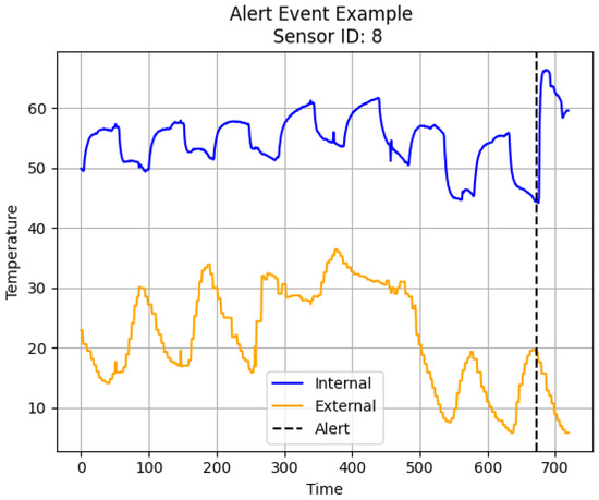
Figure 1.
Example of an alert event. The black dotted line denotes the time of an alert.
In order for this program to be effective, it is imperative that there is accurate information on whether a customer actually takes meaningful action in a timely manner after receiving an alert in order to avoid freeze loss. Although ideally, this information would be directly obtained from the customer, this is rarely possible in practice. As such, the effectiveness of the alert must be ascertained purely based on the observed pre-alert and post-alert time series. We refer to this analysis as intervention impact analysis. Essentially, a customer action has likely occurred if there is a large increase in post-alert temperatures that are incongruous with forecasts generated by a suitable time series model trained on pre-alert temperatures.
Since many of the IoT temperature time series exhibit non-linear behavior, methods such as Bayesian structural time series are inadequate for intervention impact analysis. Alternatively, the NARX and RLARX models are capable of learning non-linear behavior directly from the data, thus, we will use them in substitution of BSTS models for our impact analysis. Performance will be compared to both GP-NARX and GP-RLARX models.
5.2. Results
Once again, we apply the TP-NARX and TP-RLARX models to each alert event in our dataset and then compare the results to the GP-NARX and GP-RLARX models. For each model, we use one of four covariance kernels: radial basis function (RBF), Matérn , Matérn , or Ornstein–Uhlenbeck (OU). Outdoor (external) temperature is the only exogenous predictor used in the experiment.
Figure 2 and Figure 3 depict the forecasts for the GP-RLARX and TP-RLARX models with RBF kernel on the same alert event. As expected, the point estimates (red lines) are similar for both models; however, the predictive interval (red shaded areas) for TP-RLARX is slightly wider. For the results depicted in Figure 2 and Figure 3, the average difference between the 0.025 quantile and 0.975 quantile for GPRLARX is , whereas the average difference between the 0.025 quantile and 0.975 quantile for TPRLARX is . The wider predictive interval of TP-RLARX means that our decision on whether a customer has taken appreciable action will be more conservative. Firms wishing to be more conservative in assessing customer behavior or those with noisier time series data might prefer the TP-RLARX model.
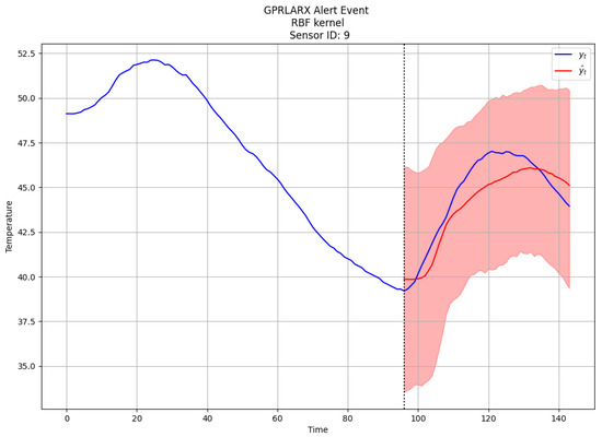
Figure 2.
Forecasts for GP-RLARX.
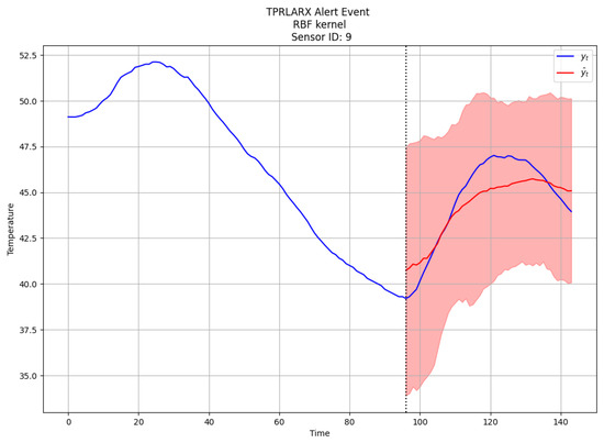
Figure 3.
Forecasts for TP-RLARX.
Furthermore, Table 3 shows the root mean squared error (RMSE), symmetric mean absolute percentage error (sMAPE), and continuous ranked probability score (CRPS) [33] for each combination of model and kernel. Each metric is calculated by averaging the metrics for each alert event within each model combination. In addition, Table 3 also gives CPU times for each model. Overall, we find that the TP-RLARX model using the Ornstein–Uhlenbeck kernel provides the best average RMSE, followed by the TP-NARX using the Matérn kernel. Furthermore, we find that the GP-RLARX models give considerably worse performance than both TP-NARX and TP-RLARX models, regardless of kernel.
Table 3.
Forecast metrics and CPU times.
5.3. Intervention Impact Analysis and Interpretation
For each alert event in this experiment, we are given a label indicating whether a panel of domain experts believed the customer took corrective action based on visual inspection of time series plots similar to Figure 1. If a majority of experts thought that action had been taken, an alert was labeled as “Action”, indicating that appreciable customer action likely occurred; otherwise, it was labeled as “No Action”. In the absence of observed labels, this is the closest approximation to the ground truth that we have and constitutes the benchmark we will compare against.
Due to this inherently biased labeling scheme, the labels we have are more aptly described as “pseudo-labels” in that they do not represent an objective truth. For alerts that experts labeled as “No Action”, we find that there is a high degree of correspondence between the model and expert labels, as indicated in Table 4. This result is unsurprising, as it is quite obvious to both experts and the models when no action has been taken because the observed internal temperature will remain flat or even decrease after the alert. Conversely, for instances labeled “Action” by experts, every model is likely to disagree, as shown in Table 4. This is attributable to the fact that whenever post-alert temperatures experience a sharp positive increase, human labelers are biased towards labeling it an action, regardless of the historical time series behavior or its correlation with the exogenous predictor. For example, Figure 4 shows an alert event labeled as “Action” by domain experts; however, there is clearly a strong, positive correlation between the internal and external temperatures that appears to instigate the increase in post-alert internal temperature. Furthermore, the post-alert increase in the response variable is quite modest and is congruent with pre-intervention temperature levels. Unsurprisingly, every possible combination of model and kernel tested returns a decision of “No Action” for this alert.
Table 4.
Confusion matrices for each model (RBF kernel).
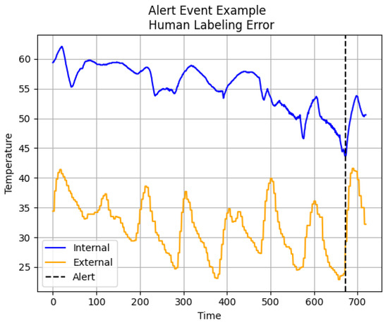
Figure 4.
Alert event mislabeled by human labelers as “Action”.
Indeed, the results of the impact analysis are congruent with our goals in that the models are far more conservative in assessing customer intervention. Expert opinion is that customers typically do not take action, so it is desirable to have models that require a large shift in post-alert behavior in order to declare an alert event as having been addressed. To that end, the RLARX models yield the best results in that they are both highly unwilling to assume an intervention has been successful without significant evidence.
6. Conclusions
In this paper, we have proposed extensions to both the GP-NARX and GP-RLARX models by replacing the GP functional prior with a Student-t process prior. The goal is to use these models as underlying forecasting models for intervention impact analysis of IoT temperature data streams. We have demonstrated that the TP-NARX and TP-RLARX models provide improved forecasting accuracy relative to the GP-NARX and GP-RLARX models. Furthermore, we have shown that the TP-RLARX model has the desirable trait of being more conservative, relative to both the GP models and human labelers, in declaring that an intervention was effective in instigating appreciable customer action in Section 5. As such, the TP-RLARX model is preferable in impact analyses where the ground truth is not necessarily known and there is a high cost associated with false positives.
The analysis performed here opens several avenues for future research. First, it would be interesting to apply the same Student-t process extension to Gaussian process state space models, such as those presented in [34,35,36], and compare their performance with models presented in this research. Furthermore, a comparison of our model with parametric non-linear time series models, such as the deep state space framework proposed in [37], would also be a worthwhile endeavor. The authors intend to explore these ideas in future research.
Author Contributions
Conceptualization, P.T., N.R. and N.L.; methodology, P.T., N.R. and N.L.; writing, reviewing and editing, P.T., N.R. and S.R. All authors have read and agreed to the published version of the manuscript.
Funding
This research received no external funding.
Data Availability Statement
Data are contained within the article.
Acknowledgments
The authors gratefully acknolwedge the support provided by Hartford Steam Boiler in providing the IoT sensor data used in this paper.
Conflicts of Interest
Patrick Toman and Nathan Lally were employed by the company Hartford Steam Boiler. The remaining authors declare that the research was conducted in the absence of any commercial or financial relationships that could be construed as a potential conflict of interest.
References
- Brockwell, P.J.; Davis, R.A. Introduction to Time Series and Forecasting; Springer: Berlin/Heidelberg, Germany, 2016. [Google Scholar]
- Abraham, B. Intervention analysis and multiple time series. Biometrika 1980, 67, 73–78. [Google Scholar] [CrossRef]
- Shumway, R.H.; Stoffer, D.S.; Stoffer, D.S. Time Series Analysis and its Applications; Springer: Berlin/Heidelberg, Germany, 2000; Volume 3. [Google Scholar]
- Van den Brakel, J.; Roels, J. Intervention analysis with state-space models to estimate discontinuities due to a survey redesign. Ann. Appl. Stat. 2010, 4, 1105–1138. [Google Scholar] [CrossRef][Green Version]
- Scott, S.L.; Varian, H.R. Predicting the present with Bayesian structural time series. Int. J. Math. Model. Numer. Optim. 2014, 5, 4–23. [Google Scholar] [CrossRef]
- Brodersen, K.H.; Gallusser, F.; Koehler, J.; Remy, N.; Scott, S.L. Inferring causal impact using Bayesian structural time-series models. Ann. Appl. Stat. 2015, 9, 247–274. [Google Scholar] [CrossRef]
- Schmitt, E.; Tull, C.; Atwater, P. Extending Bayesian structural time-series estimates of causal impact to many-household conservation initiatives. Ann. Appl. Stat. 2018, 12, 2517–2539. [Google Scholar] [CrossRef]
- Kurz, C.F.; Rehm, M.; Holle, R.; Teuner, C.; Laxy, M.; Schwarzkopf, L. The effect of bariatric surgery on health care costs: A synthetic control approach using Bayesian structural time series. Health Econ. 2019, 28, 1293–1307. [Google Scholar] [CrossRef]
- Ön, Z.B.; Greaves, A.; Akçer-Ön, S.; Özeren, M.S. A Bayesian test for the 4.2 ka BP abrupt climatic change event in southeast Europe and southwest Asia using structural time series analysis of paleoclimate data. Clim. Chang. 2021, 165, 1–19. [Google Scholar] [CrossRef]
- Toman, P.; Soliman, A.; Ravishanker, N.; Rajasekaran, S.; Lally, N.; D’Addeo, H. Understanding insured behavior through causal analysis of IoT streams. In Proceedings of the 2023 6th International Conference on Data Mining and Knowledge Discovery (DMKD 2023), Chongqing, China, 24–26 June 2023. [Google Scholar]
- Williams, C.K.; Rasmussen, C.E. Gaussian Processes for Machine Learning; MIT Press: Cambridge, MA, USA, 2006; Volume 2. [Google Scholar]
- Mattos, C.L.C.; Damianou, A.; Barreto, G.A.; Lawrence, N.D. Latent autoregressive Gaussian processes models for robust system identification. IFAC-PapersOnLine 2016, 49, 1121–1126. [Google Scholar] [CrossRef]
- Shah, A.; Wilson, A.; Ghahramani, Z. Student-t processes as alternatives to Gaussian processes. In Proceedings of the Artificial Intelligence and Statistics, PMLR, Reykjavik, Iceland, 22–25 April 2014; pp. 877–885. [Google Scholar]
- Solin, A.; Särkkä, S. State space methods for efficient inference in Student-t process regression. In Proceedings of the Artificial Intelligence and Statistics, PMLR, San Diego, CA, USA, 9–12 May 2015; pp. 885–893. [Google Scholar]
- Meitz, M.; Preve, D.; Saikkonen, P. A mixture autoregressive model based on Student’st—Distribution. Commun.-Stat.-Theory Methods 2023, 52, 499–515. [Google Scholar] [CrossRef]
- Snelson, E.; Ghahramani, Z. Sparse Gaussian processes using pseudo-inputs. In Proceedings of the Advances in Neural Information Processing Systems, Vancouver, BC, Canada, 5–8 December 2005; Volume 18. [Google Scholar]
- Titsias, M. Variational learning of inducing variables in sparse Gaussian processes. In Proceedings of the Artificial Intelligence and Statistics, PMLR, Clearwater Beach, FL, USA, 16–18 April 2009; pp. 567–574. [Google Scholar]
- Hensman, J.; Fusi, N.; Lawrence, N.D. Gaussian processes for big data. arXiv 2013, arXiv:1309.6835. [Google Scholar]
- Hensman, J.; Matthews, A.; Ghahramani, Z. Scalable variational Gaussian process classification. In Proceedings of the Artificial Intelligence and Statistics, PMLR, San Diego, CA, USA, 9–12 May 2015; pp. 351–360. [Google Scholar]
- Blei, D.M.; Kucukelbir, A.; McAuliffe, J.D. Variational inference: A review for statisticians. J. Am. Stat. Assoc. 2017, 112, 859–877. [Google Scholar] [CrossRef]
- Girard, A.; Rasmussen, C.E.; Quinonero-Candela, J.; Murray-Smith, R.; Winther, O.; Larsen, J. Multiple-step ahead prediction for non linear dynamic systems–a Gaussian process treatment with propagation of the uncertainty. Adv. Neural Inf. Process. Syst. 2002, 15, 529–536. [Google Scholar]
- Girard, A. Approximate Methods for Propagation of Uncertainty with Gaussian Process Models; University of Glasgow (United Kingdom): Glasgow, UK, 2004. [Google Scholar]
- Groot, P.; Lucas, P.; Bosch, P. Multiple-step time series forecasting with sparse gaussian processes. In Proceedings of the 23rd Benelux Conference on Artificial Intelligence, Gent, Belgium, 3–4 November 2011. [Google Scholar]
- Gutjahr, T.; Ulmer, H.; Ament, C. Sparse Gaussian processes with uncertain inputs for multi-step ahead prediction. IFAC Proc. Vol. 2012, 45, 107–112. [Google Scholar] [CrossRef]
- Bijl, H.; Schön, T.B.; van Wingerden, J.W.; Verhaegen, M. System identification through online sparse Gaussian process regression with input noise. IFAC J. Syst. Control 2017, 2, 1–11. [Google Scholar] [CrossRef]
- Titsias, M.; Lawrence, N.D. Bayesian Gaussian process latent variable model. In Proceedings of the Thirteenth International Conference on Artificial Intelligence and Statistics, Sardinia, Italy, 13–15 May 2010; JMLR Workshop and Conference Proceedings. pp. 844–851. [Google Scholar]
- Xu, Z.; Kersting, K.; Von Ritter, L. Stochastic Online Anomaly Analysis for Streaming Time Series. In Proceedings of the IJCAI, Melbourne, Australia, 19–25 August 2017; pp. 3189–3195. [Google Scholar]
- Uchiyama, Y.; Nakagawa, K. TPLVM: Portfolio Construction by Student’st-Process Latent Variable Model. Mathematics 2020, 8, 449. [Google Scholar] [CrossRef]
- Peng, C.Y.; Cheng, Y.S. Student-t processes for degradation analysis. Technometrics 2020, 62, 223–235. [Google Scholar] [CrossRef]
- Lee, H.; Yun, E.; Yang, H.; Lee, J. Scale mixtures of neural network Gaussian processes. arXiv 2021, arXiv:2107.01408. [Google Scholar]
- Ranganath, R.; Gerrish, S.; Blei, D. Black box variational inference. In Proceedings of the Artificial Intelligence and Statistics, PMLR, Reykjavik, Iceland, 22–25 April 2014; pp. 814–822. [Google Scholar]
- Bingham, E.; Chen, J.P.; Jankowiak, M.; Obermeyer, F.; Pradhan, N.; Karaletsos, T.; Singh, R.; Szerlip, P.; Horsfall, P.; Goodman, N.D. Pyro: Deep Universal Probabilistic Programming. J. Mach. Learn. Res. 2018, 20, 973–978. [Google Scholar]
- Gneiting, T.; Raftery, A.E. Strictly proper scoring rules, prediction, and estimation. J. Am. Stat. Assoc. 2007, 102, 359–378. [Google Scholar] [CrossRef]
- Frigola, R.; Chen, Y.; Rasmussen, C.E. Variational Gaussian process state-space models. In Proceedings of the Advances in Neural Information Processing Systems, Montreal, QC, Canada, 8–13 December 2014; Volume 27. [Google Scholar]
- Doerr, A.; Daniel, C.; Schiegg, M.; Duy, N.T.; Schaal, S.; Toussaint, M.; Sebastian, T. Probabilistic recurrent state-space models. In Proceedings of the International Conference on Machine Learning, PMLR, Stockholm, Sweden, 10–15 July 2018; pp. 1280–1289. [Google Scholar]
- Curi, S.; Melchior, S.; Berkenkamp, F.; Krause, A. Structured variational inference in partially observable unstable Gaussian process state space models. In Proceedings of the Learning for Dynamics and Control, PMLR, Berkeley, CA, USA, 11–12 June 2020; pp. 147–157. [Google Scholar]
- Krishnan, R.; Shalit, U.; Sontag, D. Structured inference networks for nonlinear state space models. In Proceedings of the AAAI Conference on Artificial Intelligence, San Francisco, CA, USA, 4–9 February 2017; Volume 31. [Google Scholar]
Disclaimer/Publisher’s Note: The statements, opinions and data contained in all publications are solely those of the individual author(s) and contributor(s) and not of MDPI and/or the editor(s). MDPI and/or the editor(s) disclaim responsibility for any injury to people or property resulting from any ideas, methods, instructions or products referred to in the content. |
© 2023 by the authors. Licensee MDPI, Basel, Switzerland. This article is an open access article distributed under the terms and conditions of the Creative Commons Attribution (CC BY) license (https://creativecommons.org/licenses/by/4.0/).