Article

CCrFS: Combine Correlation Features Selection for Detecting Phishing Websites Using Machine Learning

by
Jimmy Moedjahedy
1,*,
Arief Setyanto
2,*,
Fawaz Khaled Alarfaj
3 and
Mohammed Alreshoodi
4
1
Computer Science Department, Universitas Klabat, Minahasa Utara 95371, Indonesia
2
Magister of Informatics Engineering, Universitas AMIKOM Yogyakarta, Yogyakarta 55281, Indonesia
3
Department of Computer and Information Sciences, Imam Mohammad Ibn Saud Islamic University, Riyadh 11564, Saudi Arabia
4
Unit of Scientific Research, Applied College, Qassim University, Buraydah 52362, Saudi Arabia
*
Authors to whom correspondence should be addressed.
Future Internet 2022, 14(8), 229; https://doi.org/10.3390/fi14080229
Submission received: 16 June 2022 / Revised: 22 July 2022 / Accepted: 23 July 2022 / Published: 27 July 2022
(This article belongs to the Section Big Data and Augmented Intelligence)

Abstract

:
Internet users are continually exposed to phishing as cybercrime in the 21st century. The objective of phishing is to obtain sensitive information by deceiving a target and using the information for financial gain. The information may include a login detail, password, date of birth, credit card number, bank account number, and family-related information. To acquire these details, users will be directed to fill out the information on false websites based on information from emails, adverts, text messages, or website pop-ups. Examining the website’s URL address is one method for avoiding this type of deception. Identifying the features of a phishing website URL takes specialized knowledge and investigation. Machine learning is one method that uses existing data to teach machines to distinguish between legal and phishing website URLs. In this work, we proposed a method that combines correlation and recursive feature elimination to determine which URL characteristics are useful for identifying phishing websites by gradually decreasing the number of features while maintaining accuracy value. In this paper, we use two datasets that contain 48 and 87 features. The first scenario combines power predictive score correlation and recursive feature elimination; the second scenario is the maximal information coefficient correlation and recursive feature elimination. The third scenario combines spearman correlation and recursive feature elimination. All three scenarios from the combined findings of the proposed methodologies achieve a high level of accuracy even with the smallest feature subset. For dataset 1, the accuracy value for the 10 features result is 97.06%, and for dataset 2 the accuracy value is 95.88% for 10 features.

1. Introduction

Phishing is a sort of fraud that is one of the greatest threats on the Internet; it refers to false webpages that look and behave like actual webpages. Cybercriminals typically prey on individuals who lack essential digital security awareness through social engineering [1]. The objective is to dupe people into transmitting sensitive data such as their username, password, bank account number, or credit card number [2]. This form of crime can jeopardize users’ and organizations’ credibility and financial security; in some situations, phishing is the initial event that can lead to economic losses and more significant disruptions [3]; it can result in millions of dollars in losses every day [4]. According to the latest quarterly report from the Anti-Phishing Working Group (APWG) [5], since early 2020, the number of recent phishing assaults has more than doubled. As reported in the third quarter of 2021, the number of new unique phishing websites detected was 730,372, representing a rise of 30 percent from the second quarter of 2021. Moreover, between years, the number of phishing websites increased. Meanwhile, according to Phislabs’s data [6], during 2019 83.9% of phishing attacked services are financial, email, cloud, payment, and SaaS.
According to Abutair & Belghith [7], no single approach or strategy can detect all phishing websites ideally. The problem is that the website’s content is liable to change, and the website’s operational lifespan is limited. Machine learning (ML) is a promising and intelligent approach. This approach detects new phishing websites by analyzing a range of indicators, better known as features. Research on this topic attempts to implement several methods and algorithms using machine learning. The Hybrid Ensemble Feature Selection method uses a Cumulative Distribution Function gradient (CDF-g) algorithm to identify the automated feature cut-off rank.
Additionally, Chiew et al. [8] employ an ensemble technique called function perturbation. Due to this approach, Random Forest (RF) outperformed Naïve Bayes (NB), JRip, PART Classifier, and Support Vector Machines (SVM). With hybrid Natural language processing (NLP) and words vector-based features, RF receives the most excellent accuracy rating [9]. Furthermore, Nazz [10] uses a way that ranks the features based on the maximum variance using Principal Component Analysis (PCA). Next, Nazz applies RF, SVM, and Logistic Regression (LR) machine learning algorithms; the result is RF and SVM make better performance by accuracy. Each of these studies used a unique method for selecting features. Recent dataset comes with several features, and the assumption is some researchers use 50–100% of the total features, with complex computational time. For instance, Alotaibi and Alotaibi [11] used 23 from 48 features, Naaz [10] used all the features for 49, Hutchinson et al. [12] used 16 from 30 features, Karabatak and Mustafa [13] used 27 from 30 features, and Zaini et al. [14] used 15 from 30 features
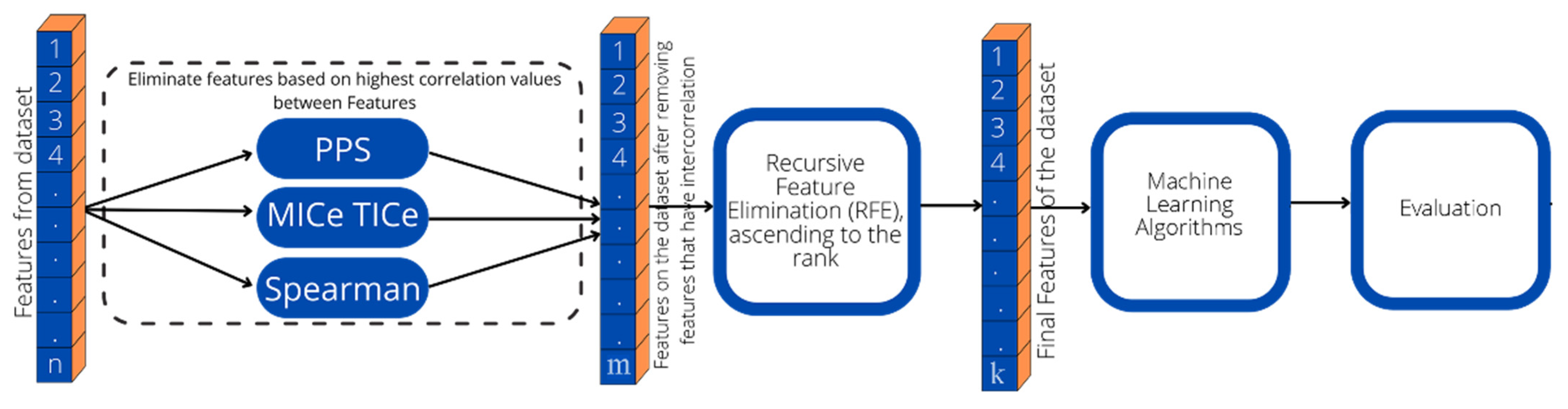
This paper’s hypothesis is that reducing low-impact features lead to simpler compu-tation with an insignificant decline in the recognition rate for the web phishing dataset. In this paper, three scenarios of feature selection followed by machine learning classification. Hence, the objectives and contributions of this paper are to propose the optimal feature selection scenario for detecting phishing websites using machine learning. We observe feature selection, and recursive feature elimination by gradually decreasing and making new subset features. Additionally, this paper conducts a comparative analysis of three correlation methods combined with a machine learning algorithm: Spearman, Power Predictive Score (PPS), and Maximal Information Coefficient (MICe) with Total Information Coefficient (TICe) on selecting features from a dataset. Moreover, a performance comparison of four Random Forest (RF), Support Vector Machine (SVM), Decision Tree (DT) and AdaBoost algorithms on selected features is evaluated.
The remaining paper is organized as follows: the second section discusses material and methods, the result is presented in Section 3, Section 4 presents the discussion, and we draw our conclusion in Section 5.

2. Materials and Methods

2.1. Data

This study utilized two public datasets; Tan’s [15] for the first dataset and Hannousse and Yahiouche [16] for the second dataset. We use this dataset because some studies on similar topics use it, such as Chiew et al. [8] on 2019, Khan et al. [17] on 2020, Dangwal and Moldova [18] on 2021, Al-Sareem et al. [19] on 2021, and Haynes et al. [20] on 2021.The first dataset selected phishing websites with the PhishTank and OpenPhish URLs and legitimate websites with the Alexa and General Archives URLs. For building the dataset, Tan gathered webpages in two different sessions between January and May and the other session in May and June for two years. The GNU Wget utility and Python programs automatically grab webpages from those two sessions. Apart from entire HTML texts, these datasets download associated resources—for example, images, CSS, and JavaScript—to guarantee that all downloaded webpages appear correctly in the browser.
The downloaded dataset is further processed to eliminate broken webpages that failed to load or sites that returned an Error 404 in phishing and legal datasets. Additionally, screenshots of each webpage are preserved for examination and filtering purposes. There are 48 features on this dataset, consisting of 10.000 data, balance for phishing and non-phishing, as seen in Table 1. The second dataset was built on 2021 and gathered URLs for the non-phishing dataset with Alexa and Yandex by crawling URLs from the top domain listed. URLs Phishing data are collected from PhisTank and OpenPhish by removing duplicates and URL that are not active anymore. Document Object Model is used for limited lifetime URLs and stores the data on a different file. There are 87 features on this dataset, and it consists of 11.430 data, balance for phishing and non-phishing. The dataset is divided into 70%, 30% for training and testing purposes.

2.2. Correlation

According to Susanti et al. [21], correlation analysis is a statistical approach used to determine the strength of a relationship between two variables or features. Additionally, this analysis assesses the direction and degree of correlations between variables or features. There are various correlation measures, the first being Spearman’s product-moment. Because it can quantify correlations on interval scales and ratios, this measure is sometimes referred to as parametric statistics. By comparison, other correlation coefficients, such as the spearman rank correlation coefficient, the Kendall correlation coefficient, and the gamma correlation coefficient, are referred to as nonparametric statistics.
Other research on correlation measurement includes those by D. N. Reshef et al. [22], who introduced a method called the Maximal Information Coefficient (MIC). As Simon & Tibshirani [23] observe, MIC is both popular and contentious; it is asserted that MIC lacks state-of-the-art. Researchers enhanced and refined their study with Reshef et al. [24] and Reshef et al. [25], which is a combination approach of MIC and Total Information Coefficient (TIC). Their strategy resulted in establishing a library, which was explored in works by Albanese et al. [26]. Wetschoreck et al. [27] also proposed the Power Predictive Score (PPS) method for assessing the level of relationships. This method arose due to various problems with correlation; there are some cases of relationships that are not found when using conventional correlation methods. This method is open-source, and they provide a library that can be downloaded and used for free.
This study used correlation to determine the correlation between features as the preliminary stages in eliminating the feature. At this stage, the correlation value between two features is rated, and then ten features with a high correlation value between features are eliminated. This method, also known as Correlation Based Feature Selection (CSF), evaluates more than one attribute and analyzes the relationship between features. In CSF, a good feature combination has substantially linked characteristics with output but not with one another [28]. Eliminating correlation between features from existing features is expected to result in unique features. Whitley et al. [29] define multicollinearity as the presence of a strong relationship between two or more variable predictors. According to Senawi et al. [30], feature selection is a process that entails identifying the most meaningful subset of characteristics for targeted concepts by excluding unnecessary features. Besides that, it can result in decision-making errors, but it can also jeopardize the legitimacy of the conclusions or outcome. The most straightforward method for determining this is building and examining correlation matrix tables.

2.3. Feature Selection

Feature selection is an activity to remove irrelevant features; the selection of features may be accomplished in two methods. The first is to rank features according to several criteria and then choose the top k features. The second approach is to select a minimal selection of characteristics without investigating performance degradation. In other words, the subset selection method may decide the number of factors to be picked automatically. In comparison, the feature rating algorithm must rely on a predefined threshold to determine the existence of a feature [31]. There are various types of feature selection, such as traditional, hybrid, and ensemble. Scikit, Boruta, MLFeaturesSelection, ITMO FS, ReBATE, MLxtend, Caret, and MLR are libraries that are frequently used for this type of study. According to studies by Pilnenskiy and Smetannikov [32], ITMO FS has superior and quicker performance.
This study chose the last ten features using Recursive feature elimination for the last stage. RFE is based on recursively developing a model by deleting features, modelling the model with the remaining features, and modelling the model’s correctness. It is a greedy optimization technique for discovering the best subset of attributes and then ranking them based on their elimination period [33]. In other words, the goal behind RFE is to train a model using all of the features in the dataset and then delete one feature at a time using recursive train models. This procedure is continued until the dataset’s components are depleted. After the process, it is possible to determine the relative value of each attribute [34].

2.4. Related Works

The studies described have a relationship with the study undertaken in feature selection. Similar to reference research by Chiew et al. [8], this study presents a novel framework for selecting Hybrid Ensemble Feature Selection (HEFS) features. The existing characteristics are then eliminated using HEFS, leaving ten baseline features. A test involving ten baseline features showed that random forest outperformed the accuracy of the other five machine learning algorithms, which was 94.6%. The subsequent study was conducted by Rao and Pais [35]. They proposed a classification model based on heuristic features taken from URLs, source code, and third-party services obtained from the analysis with eight machine learning algorithms. Random forest outperformed the accuracy value by 99.31% of the first experiment comparing eight machine learning methods. In the second experiment comparing principal component analysis (PCA-RF) with oblique Random Forests (oRFs), PCA-RF had a higher accuracy rating of 99.551%.
Salihovicd et al. [36] utilized the UCI phishing dataset to test the list of spam and phishing using six machine learning algorithms. They then conducted three software experiments: the first without changing the dataset, the second with BestFirst + CfsSubsEvaluation, and the third with Ranker + PrincipalComponents Optimization, WEKA. Random forest outperformed other machine learning algorithms on the first, second, and third trials with phishing accuracy scores of 97.26%, 94.77%, and 97.33%, respectively. Sahingoz et al. [9] researched the detection of phishing websites using random forests. Based on the results of testing seven algorithms, they discovered that only one algorithm, Random Forest combined with NLP, produced the best results, achieving an accuracy rate of 97.98%. A. Butnaru et al. [37] employed five supervised machine learning methods, including NB, DT, RF, SVM, and MLP, on a 100,315-dataset. The features utilized are a combination of ten features that are typically employed in this type of study and the two new features proposed by the authors. The hyperparameter tuning approach yields just three of the four features, namely RF, SVM, and MLP, with great performance values.
Alotaibi & Alotaibi [11] presented two approaches for selecting and eliminating features: consensus and majority voting. They use two datasets to evaluate the method. Consensus provided 17 features from the first dataset, while most votes yielded 23 features. For the second dataset, consensus yields three features, while majority voting yields thirteen. Voting is the approach with the highest accuracy, with a value of 98.63%. Haynes et al. [20] conducted similar research utilizing Artificial Neural Network (ANN), DT, Gaussian NB, Gradient Boosting (GB), KNN, RF, SVC, and SV. They also used three feature selection strategies, including URL and HTML based, URL based only, Transformer (BERT, ELECTRA) NLP. The BERT and ELECTRA methods using ANN outperform others. Previous similar research was undertaken by Al-Sarem et al. [19]. They use a genetic algorithm (GA) to optimize the parameters of several ensemble machine learning algorithms, such as XGBoost, LightGBM, random forests, AdaBoost, GB, and Bagging. The optimized classifiers were then ranked, and the three top models were selected as the foundational classifiers for a stacking ensemble technique. The trials were conducted using two datasets of phishing websites. In the first dataset, the stacking ensemble approach yields an accuracy value of 97.16%, whereas, in the second dataset, the accuracy value is 98.50%.
Table 2 provides a brief description of the associated works. The research listed is related to the work done on feature selection and machine learning methods. According to the researchers’ findings, the machine learning algorithm that outperforms others is RF [8,9,35,36]. As a result, the method employed in this work is the RF algorithm.

2.5. Methods

The analytic approach of this method is removing features from the two datasets in two steps. Firstly, eliminate intercorrelation between features using three scenarios, Pearson, MICe TICe, and PPS, and remove ten characteristics with the highest correlation value ranking, the remaining features will process in the second round with recursive feature elimination (RFE). Secondly, removing other features gradually by the ranked using RFE, as shown in Figure 1. Then, the dataset is subjected to machine learning tests utilizing Random Forest (RF), Decision Tree (DT), AdaBoost, and Support Vector Machine (SVM). As shown by this methodology, three scenarios are conducted. The first scenario is PPS + RFE, the second scenario is MICe TICe + RFE and the third use Spearman + RFE.
In Figure 1, n represents the number of full features, m the remaining features after the first removal using inter-features correlation, and k represents the remaining features after recursive elimination.

2.5.1. Scenario Using PPS + RFE

  • Step one: Choosing an algorithm; By default, this method computes results using a decision tree. A decision tree classifier will be used when obtaining data with categorical values. The decision tree regressor will then be used when numerical values are obtained. Data pre-processing: Use Label Encoding if the column whose value will be predicted or the target column has a definite value. However, if the column that denotes the alias value of the feature column has a substantial value, a one-hot encoding should be used. The metric value for evaluation: F1 score weights will be used as an evaluation metric if the chosen method is a classification method. F1 scores range from 0 to 1 on a scale of 1 to 10. The PPS value between two features is rated at this stage, and then ten features with a high correlation value between features are eliminated.
  • Step two: After deleting ten features, there are 38 remainings for dataset 1 and 77 for dataset 2. The remaining characteristics are obtained by conducting a ranking search using RFE with python sci-kit-learn and selecting rankings 1 to 10 by gradually reducing features.
  • Step three: The highest-ranked features are evaluated for accuracy using the RF algorithm.

2.5.2. Scenario Using MICe TICe + RFE

  • Step one: Using the technique illustrated in Figure 2, search for MICe TICe values in 48 and 87 existing features. Additionally, the TICe value for each pair of x, y features was determined using p-values, followed by a twofold correction test to get the MICe value for the existing feature pair. At this stage, the MICe TICe value between two features is rated, and then ten features with a high correlation value between features are eliminated. Eliminating the ten features with the highest values has a negligible effect on the output feature. Because there are up to 10,000 samples, the parameter utilized is 0.45 [26].
  • Step two: After deleting ten features, there are 38 remainings for dataset 1 and 77 for dataset 2. The remaining characteristics are obtained by conducting a ranking search using RFE with python sci-kit-learn and selecting rankings 1 to 10 by gradually reducing features.
  • Step three: The highest-ranked features are evaluated for accuracy using the RF algorithm.

2.5.3. Scenario Using Spearman + RFE

  • The first step is to find Spearman correlation coefficients ranging from 0 to 1 for each of the 48 features in the dataset. Furthermore, the Spearman correlation value is determined using MICtools provided by [26]. Then, depending on the correlation value’s results, issue ten features. The Spearman rank correlation coefficient is calculated by first rating the X elements in the paired sample data from 1 to n and then ranking the Y elements separately from one to n, assigning rank 1 to the minor component and n to the largest while retaining the original pairings. As a consequence, [rank (Xi), rank (Yi)] pairings are obtained. Then, compute a difference d equal to the difference between the X and Y variables’ ranks for each pair. As mentioned in Equation (1), the test statistic, rs, is defined as a function of the sum of squares of these differences, d [38]. At this stage, the correlation value between two features is rated, and then ten features with a high correlation value between features are eliminated.
r s = 1 6 i = 1 n d i 2 ( n 3 n )
2.
Step two: After deleting ten features, there are 38 remaining features for dataset 1 and 77 for dataset 2. The remaining characteristics are obtained by conducting a ranking search using RFE and selecting rankings 1 to 10.
3.
Step three: The ten highest-ranked features are evaluated for accuracy using the RF algorithm.

3. Results

3.1. PPS + RFE Scenario Result

After obtaining the correlation results using this method, ten features with a negligible influence on the output variable are eliminated. The value fragments are indicated in Table 3 for dataset 1 and Table 4 for dataset 2.
The deleted feature is generated by ranking the results according to the PPS correlation value that is the highest. Then, as seen in Table 5, the deleted features from those findings and their effect on the output variable for dataset 1 are RightClickDisabled, NumHash, SubdomainLevel, PctExtResourceUrls, UrlLength, SubdomainLevelRT, PathLength, NumAmpersand, NumQueryComponents, and PctExtNullSelfRedirectHyperlinksRT. For dataset 2, as seen in Table 6, the deleted features from those findings and their effect on the output variable for dataset 2 are ratio_extHyperlinks, shortest_word_path, web_traffic, char_repeat, nb_extCSS, domain_in_brand, external_favicon, domain_registration_length, links_in_tags, and ratio_intHyperlinks.

3.2. MICe TICe + RFE Scenario Result

After obtaining the correlation results using this method, ten features with a negligible influence on the output variable are eliminated. The value fragments are indicated in Table 7 for dataset 1 and Table 8 for dataset 2.
The deleted feature is generated by ranking the results according to the MICe TICe correlation value that is the highest. Then, as seen in Table 9, the deleted features from those findings and their effect on the output variable for dataset 1 are as follows: PathLevel, UrlLengthRT, PctExtResourceUrlsRT, PctExtResourceUrls, UrlLength, PathLength, QueryLength, NumAmpersand, NumQueryComponents, and PctExtNullSelfRedirectHyperlinksRT. For dataset 2, as seen in Table 10, the deleted features from those findings and their effect on the output variable for dataset 2 are are as follows: ratio_extHyperlinks, shortest_word_path, char_repeat, shortest_words_raw, nb_extCSS, nb_hyphens, ratio_extMedia, external_favicon, links_in_tags, and ratio_intMedia.

3.3. Spearman + RFE Scenario Result

After obtaining the correlation results using this method, ten features with a negligible influence on the output variable are eliminated. The value fragments are indicated in Table 11 for dataset 1 and Table 12 for dataset 2.
The deleted feature is generated by ranking the results according to the MICe TICe correlation value that is the highest. Then, as seen in Table 13, the deleted features from those findings and their effect on the output variable for dataset 1 are as follows: PathLevel, SubdomainLevel, NumNumericChars, PctExtResourceUrls, UrlLength, PathLength, QueryLength, NumAmpersand, NumQueryComponents, and NumDash. For dataset 2, as seen in Table 14, the deleted features from those findings and their effect on the output variable for dataset 2 are as follows: ratio_extHyperlinks, tld_in_path, shortest_word_path, nb_dslash, http_in_path, nb_underscore, nb_percent, char_repeat, nb_space, and shortest_words_raw.

4. Discussion

The remaining feature in each scenario then tested for classification purposes using Machine Learning algorithms.
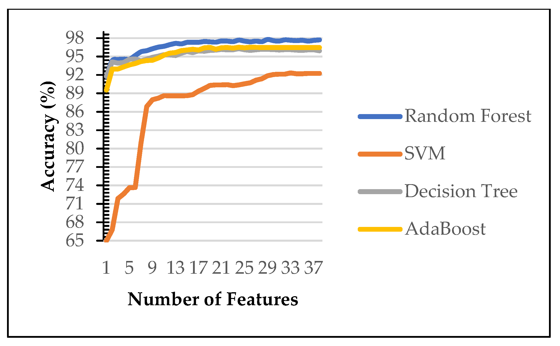
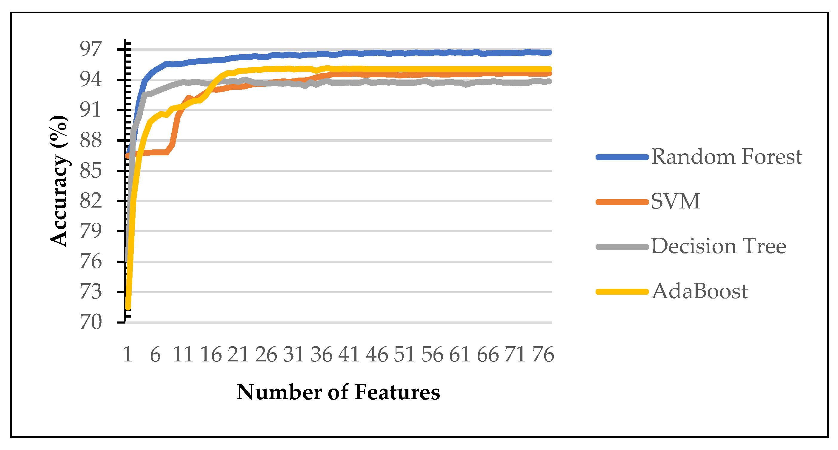
 Figure 3 and Figure 4 show the performance of machine learning algorithms on various number of selected features on the first scenario using Power Predictive score (PPS) and Recursive Feature Elimination (RFE). Random forest (RF) consistently achieves the best performance of each features subset on both dataset (blue line). Therefore, the rest of the paper evaluated on random forest algorithms only. Our finding identify RF is the best performing algorithms as reported in [8,9,36]. Therefore, the rest of the experiment was carried out on random forest (RF).
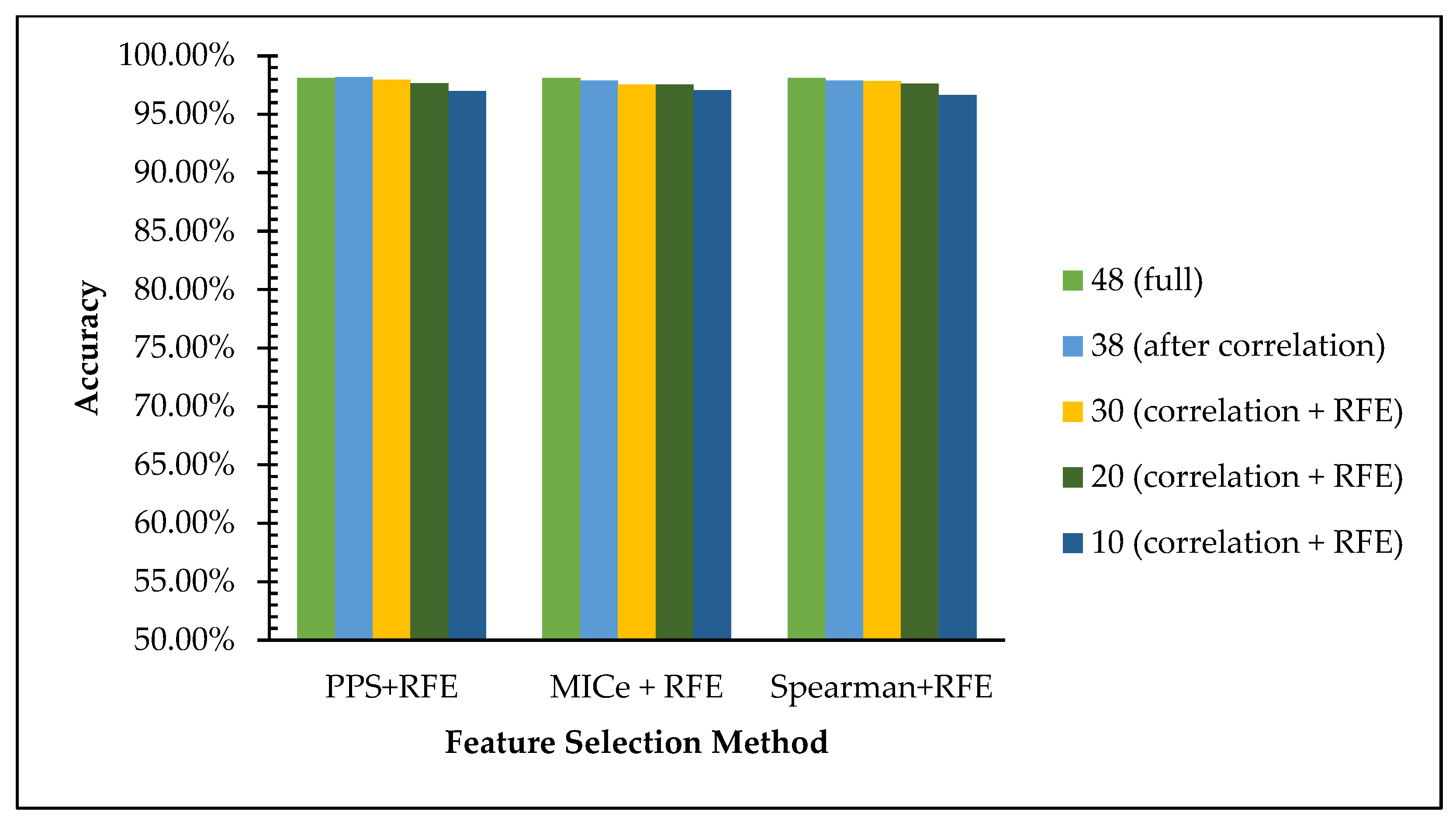
Table 15 shows the accuracy and execution time comparison of the selected features of each scenario for dataset 1. In light of the analysis of the accuracy value comparison in the graph in Figure 5, we can see that the accuracy using the Random Forest algorithm the accuracy value is maintained even with the reduction of features using three existing methods. The accuracies on the full features are achieved at 98.1%, and it declines insignificantly from 97% to 96% on 38, 30, and 20 features to 10 features. This data is in line with the hypothesis that reducing low-impact features leads to simpler computation with an insignificant decline in the web phishing dataset recognition rate.
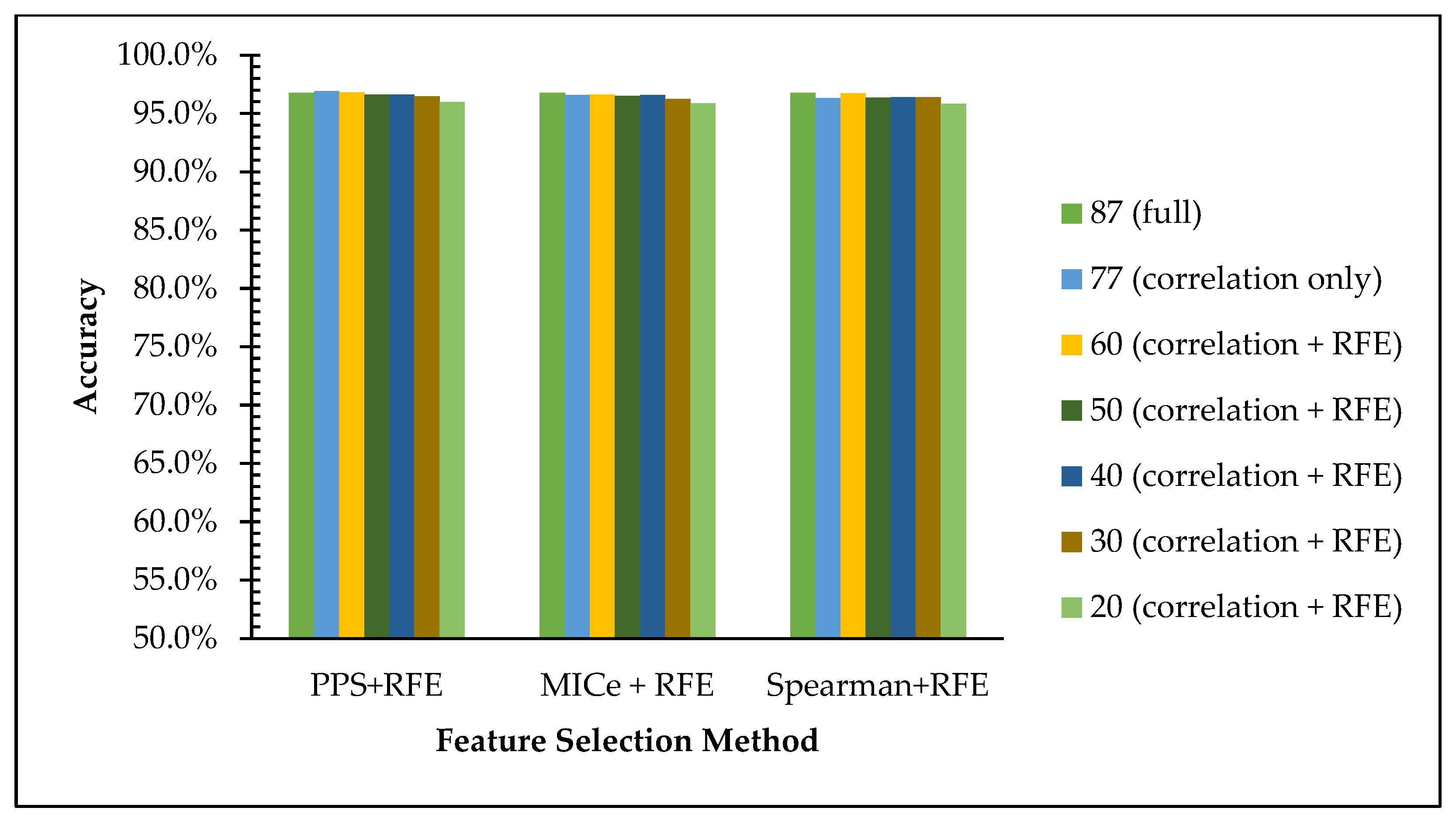
Table 16 shows the accuracy and execution time comparison of the selected features of each scenario for dataset 2. In light of the analysis of the accuracy value comparison in the graph in Figure 6, we can see that the accuracy using the Random Forest algorithm the accuracy value is maintained even with the reduction of features using three existing methods. The accuracies on the full features are achieved at 96.76%, and it declines insignificantly from 96% to 95% on 77, 60, 50, 40, 30, and 20 features to 10 features. This data is in line with the hypothesis that reducing low-impact features leads to simpler computation with an insignificant decline in the web phishing dataset recognition rate.
As we can see in Table 15 and Table 16, the accuracy is decrease as the number of features reduced, however the gap is small. For the first scenario—PPS + RFE, for example—the gap between full feature and the 10 features is less than 1% for reducing 78 features as shown on Table 16 on the second column. All experiments scenarios with two datasets shown no more than 2% gap of accuracy between full and 10 features set. The experimental result shows that reducing the features for binary classification (normal/phihing) class do not affect too much for the recognition ability of the model. Figure 5 and Figure 6 also show that reducing the number of feature do not suffer to much on recognition rate.
To decide the class, machine learning algorithms do not need to calculate all the impact of each feature in input space. Not all features share the similar impact to the class label, low correlation between input variable and the class label indicate that the data less powerful to decide the class of the input. Removing low correlation input will help to speed up the classification process. This effect clearly presented in the execution time in Table 15 and Table 16 where smaller number of features need smaller amount of time.
According to Table 15 and Table 16, removing the 10 weakest features leads to a better recognition rate because involving features with low or negative correlation cause the model to learn from disrupting information. The proof that in both datasets, accuracy improved from 96.76 to 96.93 and 98.1 to 98.16 at the first removal of the 10 weakest features in dataset1 and dataset2, respectively. In the first removal of 10 features, correlation between a pair of features is evaluated. A pair of features with correlation indicates redundant information in input side. Removing one of a pair of corelated features will not suffer the recognition rate. Some of removed features with negative correlation to the target labels as shown in Table 13 and Table 14 indicate that the features do not support the output class and therefore removing those features gives positive effect to the accuracy.
Three studies on this topic utilize the same dataset, namely the Tan dataset [15]. The results of comparing the accuracy values with the number of features extracted for each study’s methodology are presented in Table 17. According to the Table 17, our method outperformed the accuracy value from another method that uses the same dataset.
Table 17 shows the achievement of our proposed approaches compared to the existing work. Refs. [8,17] utilize the Tan’s dataset [15] with similar proportion of training and testing at 70% and 30%.
There is only one study on this topic utilize the second dataset, namely the Hannousse and Yahiouche [16] dataset. The results of comparing the accuracy values with the number of features extracted for each study’s methodology are presented in Table 18. According to the Table 18, our method outperformed the accuracy value from another method that uses the same dataset.
Table 18 shows the achievement of our proposed approaches compared to the existing work. Hannousse and Yahiouche [16] utilize dataset 2 with similar proportion of training and testing at 70% and 30%. The accuracy of RF classification of 10 selected features slightly better than the result reported in [16] with more features considered in their approach.
After feature selection, we learn about what is important: redundant features on both datasets. Although both datasets have different set of data, they share some high rank features such as length of the host name, path level and the number of hyperlink. Those high ranking features remain in the 10 most important features in the final feature selection. The first 10 removed features are redundant and it was proven removing them lead to improvement of the classification performance. For example, both “nb_dots” (number of dots) and “nb_subdomains” (number of sub domain) are highly correlated since number dots (.) are the separators between domain and subdomains and therefore removing one of them will not suffer the quality of the model, since they represent the same thing.

5. Conclusions

Removal of inter-correlated features and low and negative correlation features to the output label leads to a better recognition rate of phishing dataset. The subset of phishing datasets selected with PPS+RFE scenario slightly over-performs compared to MICe TICe+RFE and Spearman+RFE. According to the experimental result, Random Forest (RF) achieves better accuracy in recognizing the phishing website in Tan’s [15] and Hannousse and Yahiouche ’s [16] dataset. Our approach to feature selection and classification using random forest achieves slightly better accuracy on Tan’s [15] dataset at 96,96% of accuracy, compared to the result reported in [7] and [18] at 94,6% and 93.7%, respectively. On Hannousse and Yahiouche’s [16] dataset, our method of feature selection and classification using random forest also produces marginally better accuracy at 97.96%. This assumes that unimportant features can be removed without the recognition rate suffering too much. Therefore, we implement feature selection. We are aware that reducing the feature will definitely reduce the amount of information and our experiment result shows that consequent although the gap between full features and minimum subset (10 features) is less than 2% of accuracy. However, as far as accuracy is concerned, the option of using dimensionality reduction such as principal component analysis (PCA) or autoencoder would be an interesting exploration. Another remaining problem of phishing is the evolving technique of phishing itself; therefore, exercising the new evidence by providing the latest dataset is always a challenge in the future.

Author Contributions

Conceptualization, J.M. and A.S.; methodology A.S. and J.M.; software, J.M.; investigation, J.M. and F.K.A.; writing—original draft preparation J.M., A.S., M.A. and F.K.A.; data curation, M.A. and F.K.A.; visualization, J.M.; validation, A.S.; supervision, A.S.; project administration, F.K.A.; funding acquisition, F.K.A.; resources, M.A. All authors have read and agreed to the published version of the manuscript.

Funding

The authors extend their appreciation to the Deanship of Scientific Research at Imam Mohammad Ibn Saud Islamic University for funding this work through Research Group no. RG-21-51-01.

Institutional Review Board Statement

Not applicable.

Informed Consent Statement

Not applicable.

Data Availability Statement

Not applicable.

Acknowledgments

The authors are grateful to LPPM Universitas Amikom Yogyakarta for their administrative and technical support.

Conflicts of Interest

The authors declare no conflict of interest.

References

  1. Alabdan, R. Phishing Attacks Survey: Types, Vectors, and Technical Approaches. Futur. Internet 2020, 12, 168. [Google Scholar] [CrossRef]
  2. Ding, Y.; Luktarhan, N.; Li, K.; Slamu, W. A keyword-based combination approach for detecting phishing webpages. Comput. Secur. 2019, 84, 256–275. [Google Scholar] [CrossRef]
  3. Alkhalil, Z.; Hewage, C.; Nawaf, L.; Khan, I. Phishing Attacks: A Recent Comprehensive Study and a New Anatomy. Front. Comput. Sci. 2021, 3. [Google Scholar] [CrossRef]
  4. Sonowal, G.; Kuppusamy, K. PhiDMA—A phishing detection model with multi-filter approach. J. King Saud Univ.-Comput. Inf. Sci. 2020, 32, 99–112. [Google Scholar] [CrossRef]
  5. APWG. Phishing Activity Trends Report 3rd Quarter 2021; Anti Phishing Working Group: Lexington, KY, USA, 2021; Available online: https://docs.apwg.org/reports/apwg_trends_report_q3_2021.pdf (accessed on 20 February 2021).
  6. Phislabs. 2019 Phishing Trends and Intelligence Report the Growing Social Engineering Threat. 2019. Available online: https://info.phishlabs.com/hubfs/2019%20PTI%20Report/2019%20Phishing%20Trends%20and%20Intelligence%20Report.pdf (accessed on 26 April 2020).
  7. Abutair, H.; Belghith, A.; AlAhmadi, S. CBR-PDS: A case-based reasoning phishing detection system. J. Ambient Intell. Humaniz. Comput. 2019, 10, 2593–2606. [Google Scholar] [CrossRef]
  8. Chiew, K.L.; Tan, C.L.; Wong, K.; Yong, K.S.; Tiong, W.K. A new hybrid ensemble feature selection framework for machine learning-based phishing detection system. Inf. Sci. 2019, 484, 153–166. [Google Scholar] [CrossRef]
  9. Sahingoz, O.K.; Buber, E.; Demir, O.; Diri, B. Machine learning based phishing detection from URLs. Expert Syst. Appl. 2019, 117, 345–357. [Google Scholar] [CrossRef]
  10. Naaz, S. Detection of Phishing in Internet of Things Using Machine Learning Approach. Int. J. Digit. Crime Forensics 2021, 13, 1–15. [Google Scholar] [CrossRef]
  11. Alotaibi, B.; Alotaibi, M. Consensus and majority vote feature selection methods and a detection technique for web phishing. J. Ambient Intell. Humaniz. Comput. 2021, 12, 717–727. [Google Scholar] [CrossRef]
  12. Hutchinson, S.; Zhang, Z.; Liu, Q. Detecting Phishing Websites with Random Forest. In International Conference on Machine Learning and Intelligent Communications, Proceedings of the Third International Conference, MLICOM 2018, Hangzhou, China, 6–8 July 2018; Lecture Notes of the Institute for Computer Sciences, Social Informatics and Telecommunications Engineering (LNICST); Springer: Cham, Switzerland, 2018; pp. 470–479. [Google Scholar] [CrossRef]
  13. Karabatak, M.; Mustafa, T. Performance comparison of classifiers on reduced phishing website dataset. In Proceedings of the 6th International Symposium on Digital Forensic and Security (ISDFS), Antalya, Turkey, 22–25 March 2018; pp. 1–5. [Google Scholar] [CrossRef]
  14. Zaini, N.S.; Stiawan, D.; Ab Razak, M.F.; Firdaus, A.; Din, W.I.S.W.; Kasim, S.; Sutikno, T. Phishing detection system using nachine learning classifiers. Indones. J. Electr. Eng. Comput. Sci. 2020, 17, 1165–1171. [Google Scholar] [CrossRef]
  15. Tan, C.L. Mendeley Data—Phishing Dataset for Machine Learning: Feature Evaluation. 2018. Available online: https://data.mendeley.com/datasets/h3cgnj8hft/1 (accessed on 13 May 2020).
  16. Hannousse, A.; Yahiouche, S. Towards benchmark datasets for machine learning based website phishing detection: An experimental study. Eng. Appl. Artif. Intell. 2021, 104, 104347. [Google Scholar] [CrossRef]
  17. Khan, S.A.; Khan, W.; Hussain, A. Phishing Attacks and Websites Classification Using Machine Learning and Multiple Datasets (A Comparative Analysis). In International Conference on Intelligent Computing, Proceedings of the 16th International Conference, ICIC 2020, Bari, Italy, 2–5 October 2020; Springer: Cham, Switzerland, 2020; pp. 301–313. [Google Scholar] [CrossRef]
  18. Dangwal, S.; Moldovan, A.-N. Feature Selection for Machine Learning-based Phishing Websites Detection. In Proceedings of the International Conference on Cyber Situational Awareness, Data Analytics and Assessment (CyberSA), Dublin, Ireland, 14–18 June 2021; pp. 1–6. [Google Scholar] [CrossRef]
  19. Al-Sarem, M.; Saeed, F.; Al-Mekhlafi, Z.; Mohammed, B.; Al-Hadhrami, T.; Alshammari, M.; Alreshidi, A.; Alshammari, T. An Optimized Stacking Ensemble Model for Phishing Websites Detection. Electronics 2021, 10, 1285. [Google Scholar] [CrossRef]
  20. Haynes, K.; Shirazi, H.; Ray, I. Lightweight URL-based phishing detection using natural language processing transformers for mobile devices. Procedia Comput. Sci. 2021, 191, 127–134. [Google Scholar] [CrossRef]
  21. Susanti, D.S.; Sukmawaty, Y.; Salam, N. Analisis Regresi dan Korelasi, 1st ed.; CV IRDH: Malang, Indonesia, 2019; pp. 49–50. [Google Scholar]
  22. Reshef, D.N.; Reshef, Y.A.; Finucane, H.K.; Grossman, S.R.; McVean, G.; Turnbaugh, P.J.; Lander, E.S.; Mitzenmacher, M.; Sabeti, P.C. Detecting Novel Associations in Large Data Sets. Science 2011, 334, 1518–1524. [Google Scholar] [CrossRef] [PubMed] [Green Version]
  23. Simon, N.; Tibshirani, R. Commen on Detection Novel Associations in Large Data Sets by Reshef et al, Science Dec 16, 2011. Science 2011, 334, 1521–1522. [Google Scholar]
  24. Reshef, D.N.; Reshef, Y.A.; Sabeti, P.C.; Mitzenmacher, M.M. An Empirical Study of Leading Measures of Dependence. arXiv 2015, arXiv:1505.02214. [Google Scholar]
  25. Reshef, Y.A.; Reshef, D.N.; Finucane, H.K.; Sabeti, P.C.; Mitzenmacher, M. Measuring dependence powerfully and equitably. J. Mach. Learn. Res. 2016, 17, 1–63. [Google Scholar]
  26. Albanese, D.; Riccadonna, S.; Donati, C.; Franceschi, P. A practical tool for maximal information coefficient analysis. GigaScience 2018, 7, 1–8. [Google Scholar] [CrossRef] [PubMed] [Green Version]
  27. Wetschoreck, F.; Krabel, T.; Krishnamurthy, S. 8080labs/ppscore: Zenodo release; Zenodo: London, UK, 2020. [Google Scholar] [CrossRef]
  28. Raza, M.S.; Qamar, U. Understanding and Using Rough Set Based Feature Selection: Concepts, Techniques and Applications; Springer: Singapore, 2017; pp. 42–45. [Google Scholar]
  29. Whitley, B.E.; Kite, M.E.; Adams, H.L. Principles of Research in Behavioral Science, 3rd ed.; Routledge: New York, NY, USA, 2013. [Google Scholar]
  30. Senawi, A.; Wei, H.-L.; Billings, S.A. A new maximum relevance-minimum multicollinearity (MRmMC) method for feature selection and ranking. Pattern Recognit. 2017, 67, 47–61. [Google Scholar] [CrossRef]
  31. Liu, H.; Motoda, H. Computational Methods of Feature Selection; CRC Press: Boca Raton, FL, USA, 2007. [Google Scholar]
  32. Pilnenskiy, N.; Smetannikov, I. Feature Selection Algorithms as One of the Python Data Analytical Tools. Futur. Internet 2020, 12, 54. [Google Scholar] [CrossRef] [Green Version]
  33. Das, S.; Cakmak, U.M. Hands-On Automated Machine Learning A Beginner’s Guide to Building Automated Machine Learning Systems Using AutoML and Python; Packt Publishing Ltd.: Birmingham, UK, 2018. [Google Scholar]
  34. Mishra, A. Machine Learning for IOS Developers; Wiley: Oxford, UK, 2020. [Google Scholar] [CrossRef]
  35. Rao, R.S.; Pais, A.R. Detection of phishing websites using an efficient feature-based machine learning framework. Neural Comput. Appl. 2019, 31, 3851–3873. [Google Scholar] [CrossRef]
  36. Salihovicd, I.; Serdavic, H.; Kevric, J. The Role of Feature Selection in Machine Learning for Detection of Spam and Phishing Attacks. In International Symposium on Innovative and Interdisciplinary Applications of Advanced Technologies (IAT); Springer: Cham, Switzerland, 2019; Volume 3, pp. 476–483. [Google Scholar] [CrossRef]
  37. Butnaru, A.; Mylonas, A.; Pitropakis, N. Towards Lightweight URL-Based Phishing Detection. Futur. Internet 2021, 13, 154. [Google Scholar] [CrossRef]
  38. Podgor, M.J.; Gibbons, J.D. Nonparametric Measures of Association. J. Am. Stat. Assoc. 1994, 89, 719. [Google Scholar] [CrossRef]
Figure 1. Feature selection and elimination approach from this method.
Futureinternet 14 00229 g001
Figure 2. Procedures for finding MICe TICe values.
Futureinternet 14 00229 g002
Figure 3. Comparison of various machine learning algorithms for dataset 1.
Futureinternet 14 00229 g003
Figure 4. Comparison of various machine learning algorithms for dataset 2.
Futureinternet 14 00229 g004
Figure 5. Comparison of all feature subset scenarios for dataset 1.
Futureinternet 14 00229 g005
Figure 6. Comparison of all feature subset scenarios for dataset 2.
Futureinternet 14 00229 g006
Table 1. Dataset information.
Dataset/CategoryFeaturesTotal DataNon-PhishingPhishingPublished
Tan [15]/URL4810.0005000 50002018
Hannousse and Yahiouche [16]/URL8711.430571557152021
Table 2. Brief description of related works.
Authors/YearDatasetNumber of FeaturesMachine Learning AlgorithmFeature Selection AlgoritmAccuracy
Rao & Pais [35]/2019Build their own dataset using Phistank and AlexaNot statedRF, J48 Tree Decision, LR, Bayesian Network (BN), SVM, Sequential Minimal Optimization (SMO), AdaBoostM1, Multi-Layer Perceptron (MLP)PCA-RF, obligate RF. PCF-RF performed the best accuracyExperiment 1: 99.3%
Experiment 2: 93.19%
Chiew et al. [8]/2019Tan [15]10PART, JRip, RF, SVM, NB, C4.5Hybrid Ensemble Feature Selection (HEFS), When HEFS is integrated with RF, the result outperforms another algorithm94.6%
Salihovic et al. [36]/2019UCIs Phishing Websites Data Set and Spam Emails Dataset10
16
RF, K-Nearest Neighbor (KNN), SVM, LR, Artificial Neural Network (ANN), NBBestFirst, CfsSubsEvaluation and Ranker, PrincipalComponents Optimization. Ranker + PrincipalComponents optimization using RF has the best accuracy97.33%
94.24%
Sahingoz et al. [9]/2019construct their own dataset40RF, DT, AdaBoost, SMO, NB, K-Star, KNNFeature reduction mechanism using Natural Language Processing (NLP) features based.
RF with NLP features outperform the other algorithms
97.98%
Alotaibi & Alotaibi [11]/2021Tan [15]23SVM, NB, AdaBoost, LightGBMConsensus and majority voting feature selection. Consensus and voting with Adaboost and LightGMB get the best result98.63%
Haynes et al. [20]/2021Shirazi Dataset15Artificial Neural Network (ANN), DT, Gaussian NB, Gradient Boosting (GB), KNN, RF, SVC, SVMURL and HTML based, URL based only, Transformer (BERT, ELECTRA) NLP. BERT and ELECTRA using ANN outperform another methodMore than 96%
Al-Sarem et al. [19] /2021UCI dataset
Tan [15]
Mendeley dataset
Not statedXGBoost, AdaBoost, RF, GradientBoost, Bagging, LightGBMEnsemble, GA-based ensemble. GA-SVM outperforms another method97.16%, 98.58%, 97.39%
Table 3. PPS value between variables for dataset 1.
NoVariable 1Variable 2PPS Value
1UrlLengthRTUrlLength1
2NumHashUrlLength1
3SubdomainLevelRTSubdomainLevel0.93
4NumAmpersandNumQueryComponents0.84
5NumHashNumAmpersand0.83
6ExtMetaScriptLinkRTPctExtResourceUrls0.76
7RightClickDisabledPctNullSelfRedirectHyperlinks0.7
8PctExtNullSelfRedirectHperlinksRTPctExtHyperlinks0.69
9UrlLengthRTPathLength0.68
10RightClickDisabledPctExtHyperlinks0.65
11PctExtResourceUrlsRTPctExtResourceUrls0.65
12FrequentDomainNameMismatch 0.63
13FrequentDomainNameMismatchPctExtResourceUrls0.63
14AbnormalExtFormActionRExtFormAction0.63
24UrlLengthRTNumDash0.42
25DomainInPathsNumDash0.42
26SubdomainLevelRTHostNameLength0.42
27PathLengthUrlLength0.41
28QueryLengthNumQueryComponents0.41
29RandomStringUrlLength0.4
Table 4. PPS value between variables on Dataset 2.
NoVariable 1Variable 2PPS Value
1domain_agedomain_in_brand0.749341935
2ratio_intHyperlinksratio_extHyperlinks0.72978711
3nb_eqnb_and0.720697676
4nb_eqnb_qm0.702171885
5longest_word_pathavg_word_path0.655215372
6shortest_word_hostnb_www0.640106706
7avg_word_pathlongest_word_path0.611298231
8char_repeatnb_www0.607295021
9longest_word_pathlongest_words_raw0.605856693
10ratio_extHyperlinksratio_intHyperlinks0.592877237
11nb_subdomainsnb_dots0.569833309
12avg_word_hostlongest_word_host0.556752327
13length_urllength_words_raw0.55302947
14length_words_rawlength_url0.529359974
37web_trafficpage_rank0.411068239
38nb_hyperlinksempty_title0.408773788
39ratio_extHyperlinksstatus0.406332414
40ratio_intHyperlinksstatus0.406029351
41ratio_intHyperlinksexternal_favicon0.403947811
42shortest_word_hostavg_word_host0.400271455
Table 5. List of removed features using PPS and their effect on the output variable for dataset 1.
Removed FeaturesEffect on the Output Variable
RightClickDisabled0.0749
NumHash0.048
SubdomainLevel0.0431
PctExtResourceUrls−0.0219
UrlLength−0.0745
SubdomainLevelRT−0.0758
PathLength−0.0761
NumAmpersand−0.0814
NumQueryComponents−0.1474
PctExtNullSelfRedirectHyperlinksRT−0.5405
Table 6. List of removed features using PPS and their effect on the output variable on dataset 2.
Removed FeaturesEffect on the Output Variable
ratio_extHyperlinks0.0834
shortest_word_path0.0744
web_traffic0.0604
char_repeat0.0147
nb_extCSS−0.0836
domain_in_brand−0.0982
external_favicon−0.1466
domain_registration_length−0.1617
links_in_tags−0.1844
ratio_intHyperlinks−0.244
Table 7. MICe TICe correlation value between features on dataset 1.
NoVariable 1Variable 2MICe TICe Value
1UrlLengthUrlLengthRT1.000
2NumQueryComponentsQueryLength0.638
3PctExtResourceUrlsExtMetaScriptLinkRT0.550
4PctExtResourceUrlsPctExtResourceUrlsRT0.549
5PctExtHyperlinksPctExtNullSelfRedirectHyperlinksRT0.508
6UrlLengthPathLength0.468
7ExtFormActionAbnormalExtFormActionR0.461
8PathLengthUrlLengthRT0.422
9NumQueryComponentsNumAmpersand0.401
10PctExtHyperlinksFrequentDomainNameMismatch0.336
11NumAmpersandQueryLength0.320
12PathLevelPathLength0.318
13PctExtResourceUrlsFrequentDomainNameMismatch0.307
14PctExtHyperlinksPctExtResourceUrls0.296
15NumDotsSubdomainLevel0.296
770NumHashInsecureForms0.0006
771TildeSymbolExtFavicon0.0006
772IpAddressDomainInSubdomains0.0006
Table 8. MICe TICe correlation value between features on dataset 2.
NoVariable 1Variable 2MICe TICe Value
1nb_dotsnb_subdomains0.93006
2ratio_intHyperlinksratio_extHyperlinks0.928648
3shortest_word_pathlongest_word_path0.857185
4shortest_word_pathavg_word_path0.857185
5longest_word_pathavg_word_path0.857185
6longest_word_hostavg_word_host0.655094
7shortest_words_rawshortest_word_path0.645462
8length_urllength_words_raw0.637978
9nb_wwwshortest_word_host0.592451
10nb_wwwchar_repeat0.591922
11longest_words_rawlongest_word_host0.582465
12ratio_intMediaratio_extMedia0.556993
13length_words_rawlongest_word_path0.556662
14length_words_rawavg_word_path0.545439
15length_words_rawshortest_word_path0.542383
2511nb_starnb_redirection0.000528
2512path_extensionempty_title0.000526
2513nb_tildewhois_registered_domain0.000515
Table 9. List of removed features using MICe TICe and their effect on the output variable on dataset 1.
Removed FeaturesEffect on the Output Variable
PathLevel0.2295
UrlLengthRT0.1695
PctExtResourceUrlsRT0.0521
PctExtResourceUrls−0.0219
UrlLength−0.0745
PathLength−0.0761
QueryLength−0.0805
NumAmpersand−0.0814
NumQueryComponents−0.1474
PctExtNullSelfRedirectHyperlinksRT−0.5405
Table 10. List of features removed using MICe TICe and their effect on the output variable on dataset 2.
Removed FeaturesEffect on the Output Variable
ratio_extHyperlinks0.0834
shortest_word_path0.0744
char_repeat0.0147
shortest_words_raw−0.0394
nb_extCSS−0.0836
nb_hyphens−0.1001
ratio_extMedia−0.1404
external_favicon−0.1466
links_in_tags−0.1844
ratio_intMedia−0.1933
Table 11. Spearman correlation value between features on dataset 1.
NoVariable 1Variable 2Spearman Value
1NumQueryComponentsQueryLength0.959329
2NumQueryComponentsNumAmpersand0.750978
3UrlLengthPathLength0.724112
4NumAmpersandQueryLength0.708677
5PathLevelPathLength0.652628
6UrlLengthNumNumericChars0.564596
7NumDashPathLength0.550183
8NumDotsSubdomainLevel0.542126
9PctExtHyperlinksPctExtResourceUrls0.520385
10UrlLengthNumDash0.501986
11PctExtResourceUrlsRTExtMetaScriptLinkRT0.487458
12PctExtResourceUrlsFrequentDomainNameMismatch0.465619
13SubdomainLevelHostnameLength0.459177
14NumNumericCharsRandomString0.457105
15RelativeFormActionAbnormalFormAction0.429697
770RandomStringPctExtResourceUrls0.000528
771NumUnderscoreMissingTitle0.000107
772PctExtHyperlinksUrlLengthRT0.000058
Table 12. Spearman correlation value between features on Dataset 2.
NoVariable 1Variable 2Spearman Value
1nb_dotsnb_subdomains0.981132
2longest_word_pathavg_word_path0.928796
3nb_qmnb_eq0.916903
4length_urllength_words_raw0.907651
5longest_word_hostavg_word_host0.878764
6length_urllongest_word_path0.831591
7ratio_intHyperlinkslinks_in_tags0.787153
8longest_words_rawavg_words_raw0.756151
9length_hostnamelongest_word_host0.748802
10nb_percentnb_space0.748207
11length_words_rawlongest_word_path0.747163
12shortest_word_pathavg_word_path0.742056
13nb_extCSSexternal_favicon0.737071
14google_indexstatus0.731171
15nb_slashlength_words_raw0.720081
2511page_rankstatus−0.546889
2512nb_hyperlinksstatus−0.551603
2513length_words_rawshortest_words_raw−0.621968
Table 13. List of removed features using Spearman and their effect on the output variable on dataset 1.
Removed FeaturesEffect on the Output Variable
PathLevel0.2295
SubdomainLevel0.0431
NumNumericChars0.0191
PctExtResourceUrls−0.0219
UrlLength−0.0745
PathLength−0.0761
QueryLength−0.0805
NumAmpersand−0.0814
NumQueryComponents−0.1474
NumDash−0.3722
Table 14. List of features removed using Spearman and their effect on the output variable on dataset 2.
Removed FeaturesEffect on the Output Variable
ratio_extHyperlinks0.08336
tld_in_path0.07915
shortest_word_path0.07436
nb_dslash0.0726
http_in_path0.07078
nb_underscore0.03809
nb_percent0.0281
char_repeat0.01473
nb_space−0.00419
shortest_words_raw−0.03936
Table 15. Feature subset accuracy and execution time on Dataset 1.
Features SubsetAccuracyExecution Time
(Second)
PPS + RFEMICe + RFESpearman + RFEPPS + RFEMICe + RFESpearman + RFE
48 (full)98.1%98.1%98.1%0.9830280.9830280.983028
38 (correlation only)98.16%97.86%97.86%0.9836810.9785570.977316
30 (correlation + RFE)97.96%97.53%97.83%0.9810950.9728500.977302
20 (correlation + RFE)97.63%97.53%97.6%0.9778350.9746910.975958
10 (correlation + RFE)96.96%97.06%96.63%0.9707030.9695390.969281
Table 16. Feature subset accuracy using Spearman on Dataset 2.
Features SubsetAccuracyExecution Time
(Second)
PPS + RFEMICe + RFESpearman + RFEPPS + RFEMICe + RFESpearman + RFE
87 (full)96.76%96.76%96.76%0.9697860.9697860.969786
77 (correlation only)96.93%96.58%96.32%0.9738090.9685640.967281
60 (correlation + RFE)96.79%96.61%96.73%0.9731660.9708150.967000
50 (correlation + RFE)96.61%96.52%96.35%0.9702550.9679710.963443
40 (correlation + RFE)96.61%96.58%96.38%0.9713770.9685640.962919
30 (correlation + RFE)96.47%96.23%96.38%0.9651710.9639050.961832
20 (correlation + RFE)95.97%95.88%95.82%0.9609690.9598100.958136
10 (correlation + RFE)95.88%95.21%95.04%0.9571090.9506170.948853
Table 17. The studies feature set and accuracy comparison on Tan’s dataset.
NoFeature TypesetFeaturesAccuracy
Chiew et al. [8]Full Features4896.17%
Baseline1094.60%
Full Features HEFS3092.40%
Baseline HEFS593.22%
Khan et al. [17]Full Features4897.87%
Using PCA3094.90%
Dangwal et al. [18]RF3093.7%
OursFull features4898.1%
PPS Correlation Only3898.16%
PPS+RFE3097.96%
PPS+RFE2097.63%
PPS+RFE1096.96%
MICe TICe Correlation Only3897.86%
MICe TICe + RFE3097.53%
MICe TICe + RFE2097.53%
MICe TICe + RFE1097.06%
Spearman Correlation Only3897.86%
Spearman + RFE3097.83%
Spearman + RFE2097.6%
Spearman + RFE1096.63%
Table 18. The studies feature set and accuracy comparison on Hannousse and Yahiouche dataset.
NoFeature TypesetFeaturesAccuracy
Hannousse and Yahiouche [16]URLs based + Content based + External features (Full features)8796.61%
URLs based + Content based8094.10%
URLs based + External features6396.65%
Content based + External features3195.13%
URLs based5691%
Content based2489.90%
External Features794.09%
OursFull features8796.76%
PPS Correlation Only7796.93%
PPS+RFE1095.58%
MICe TICe Correlation Only7796.58%
MICe TICe + RFE1095.21%
Spearman Correlation Only7796.32%
Spearman + RFE1095.04%
Publisher’s Note: MDPI stays neutral with regard to jurisdictional claims in published maps and institutional affiliations.

