Multilayer Backbones for Internet of Battlefield Things ^†

Abstract

The Internet of Battlefield Things is a newly born cyberphysical system and, even though it shares a lot with the Internet of Things and with ad hoc networking, substantial research is required to cope with its scale and peculiarities. This article examines a fundamental problem pertaining to the routing of information, i.e., the calculation of a backbone network. We model an IoBT network as a network with multiple layers and employ the concept of domination for multilayer networks. This is a significant departure from earlier works, and in spite of the huge literature on the topic during the past twenty years, the problem in IoBT networks is different since these networks are multilayer networks, thus making inappropriate all the past, related literature because it deals with single layer (flat) networks. We establish the computational complexity of our problem, and design a distributed algorithm for computing connected dominating sets with small cardinality. We analyze the performance of the proposed algorithm on generated topologies, and compare it against two—the only existing—competitors. The proposed algorithm establishes itself as the clear winner in all experiments concerning the dominating set from a size-wise and an energy-wise perspective achieving a performance gain of about 15%.

1. Introduction

The progress in IoT inevitably impacted upon the modern battlefield, which is populated by thousands of “things”, such as humans, sensors, vehicles, unmanned aerial vehicles (UAVs), aircrafts, etc. carrying out various tasks including environmental sensing, communicating, acting in isolation and/or in cooperation [1,2]. Therefore, the Internet of Battle(field) Things [1] or the Internet of Military Things (IoMT) was born, which interconnects “devices” aiming to meet multiple and diverse missions, to operate in a (semi)autonomic mode, and to execute battlefield operations supporting end-to-end control and command; its ultimate goal is to carry out a commander’s intent in a safe, responsive and resilient manner. Thus, IoBT presents at the same time all of the following significant and very challenging characteristics [3] which distinguish it from traditional IoT:

• Diversity in tasks and aims. There will be many networks operating simultaneously to achieve a particular goal, e.g., tracking, surveillance, attack.
• Operation in dynamically changing and resource starving environments. Some “devices” of the IoBT network might be energy-starving (sensors, drones), others might not have energy issues (armored vehicles), others might be obliged to travel in non-chartered territories (e.g., planes).
• Extreme device heterogeneity. IoBT networks are expected to include from tiny little sensors to some as big as armored fighting vehicles.
• High variance in network’s density and size. An IoBT network might be comprised e.g., by the cluttered network of a swarm of drones, or by the “union” of the ad hoc network of a battalion’s soldiers and the ad hoc network of a tank platoon.

The so-called assured synthesis is one of the major challenges identified for IoBT, and in particular the recruitment and network composition [3] tasks. The former task is about the discovery of cyberphysical assets, the human assets and their particularities, and also about the resilience to adversaries. The latter task is about the issue of dictating the nodes that must be considered in order for the requirements and constraints of the planned mission to be satisfied.

1.1. Related Literature

The Internet of Battlefield Things concept emerged some five years ago [1,4], and since then research is conducted in designing backbones [5,6], in designing reconfigurable and secure IoBT networks [7], in developing solutions for enemy localization [8], in controling/monitoring communication links, in combating attacks at nodes [9], in detecting malware and fake news [10,11], and in protecting human assets [12,13].

The past literature on designing backbones for routing support in wireless ad hoc networks comprises the most closely related work to the present article. This literature is literally enormous during the past two decades [14,15,16]. However, the same issue in the realm of military/IoBT networks is different; these networks are actually multilayer networks [5,7] (see Figure 1), and therefore this past literature is in principle inappropriate, because it concentrates only on single layer networks. Moreover, we showed in ([5] Theorem 1), that these algorithms usually produce suboptimal solutions in the sense that, instead of announcing as a dominator a node with a few interlayer links, they tend to announce someone with many intralayer links. Finally, the work in [17] deals with domination in multiplex networks which is a far more restricted version of multilayer networks, since interlayer links exist only between clones of the same node in different layers; moreover, that work does not establish the computational complexity of their problem.

The very first algorithm for calculating a backbone for multilayer military networks is described in [5], where a distributed backbone establishment algorithm, namely clPCI was presented. It is based on the concept of connected dominating sets (CDS). The concept of a CDS was selected for the following reasons: (a) only/mainly distributed algorithms are appropriate in the battlefield, and despite the fact that finding a Minimum CDS is a NP-complete problem even in the centralized setting, there exist some very efficient distributed algorithms for the problem; (b) the battlefield requires resilient solutions, and fortunately the scientific knowledge on how to build a multi-connected, multi-dominating CDS is quite mature [18]; and finally (c) an IoBT is composed by many energy-starving devices, and therefore energy-aware solutions (e.g., sleep scheduling) is almost mandatory; again, the theory on how to create multiple dominating sets, i.e., domatic partitions [19] is quite rich. Until before the introduction of clPCI for constructing a connected dominating set in a distributed fashion for multilayer networks, there was no prior work on the topic. This complete lack may be attributed to the mistaken assumption that a multilayer network is equivalent (from the perspective of computing a CDS) to a single layer network after ignoring layer information.

Multilayer networks have also been used in biological sciences in order to model interacting networks. In [20], $FAST\text{-}MDSM$ is developed to calculate a dominating sets in multilayer networks. However, this algorithm is centralized, and it results in an unconnected dominating set, incurring also a high computation cost because it runs as an integer programming problem (Calculating a minimum (connected) dominating set after formulating it as an integer programming model is a mature technique [21]). In conclusion, all aforementioned algorithms consider only single layer networks, with the exception of [5], and of the centralized $FAST\text{-}MDSM$ which comprises a departure from this literature.

1.2. Motivation and Work’s Contributions

In [5] we dealt with the heterogeneity of an IoBT network and modelled it as a multilayer network. We proved analytically that if we treat it as a plain union of independent subnetworks, then we do not reap efficient solutions for facilitating fast information routing. So, despite the past, very rich literature on the domination concept in ad hoc networks, the problem in IoBT networks is different, since these are multilayer networks and considering them as a single (flat) network or considering each layer in isolation and calculating dominating set produces either suboptimal or bad solutions. Therefore, the whole past literature is in principle inappropriate. Later, we incorporated in this first work energy issues [6], and we devised algorithms with fact-finding methods to address aspects of social sensing, e.g., characterize human assets/sources. We note here, that in [5] we developed distributed, communication-efficient algorithms based on the concept of node domination for choosing a set of nodes to be a backbone for a multilayer network, i.e., the IoBT network. In the biological sciences area, the work described in [20] developed centralized algorithms for computing dominating sets in multilayer networks.

Nevertheless, neither the algorithms developed in [5] (and of course in [6]) nor those developed in [20] can adequately serve the purposes of an IoBT backbone network. The main issue with the former algorithms is that they do not produce very compact network spanners, so there is plenty of room for improvement with regard to the produced connected dominating set. This is very significant if we wish to design solutions scalable to enormous IoBT networks. The two main disadvantages of the latter algorithm is its centralized nature, and thus it can not work in IoBT, and additionally because it produces unconnected spanners, and therefore it can not guarantee network-wide flow of information. Thus, our article contributes the following:

• It establishes the computation complexity (NP-completeness) of the problem of calculating a minimum connected dominating set for multilayer networks.
• It presents a new distributed algorithm, namely the Cross layer Connected Dominating Set ($CCDS$) for calculating connected dominating sets for IoBT networks, by applying an efficient mechanism to reduce the size of the dominating set.
• It enhances $FAST\text{-}MDSM$ [20] so as to produce connected dominating sets thus getting a new algorithm called $FAST\text{-}CMDSM$, and compares our proposed algorithm against the only existing competitors, namely the algorithm in [5] and $FAST\text{-}CMDSM$.

The rest of this article is organized as follows: Section 2 formulates the problem and proves its complexity, and Section 3 develops distributed solutions for it. Section 4 evaluates the competing algorithms, and  finally, Section 5 summarizes the article.

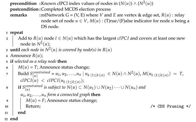
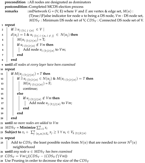
2. Formulation of the Problem

A dominating set (DS) [22] of a graph (i.e., the set of dominators) is defined as a subset of the nodes with the property that the rest of the nodes are adjacent (i.e., 1-hop neighbors) from some dominator(s). If the network induced by the DS is additionally connected, then the DS is called connected DS (CDS). In the IoBT setting, we seek for minimum CDS (MCDS), i.e., CDS with minimum cardinality. We treat an IoBT network as a multilayer network, i.e., as a multilayer graph [5,7]. We assume that there exist only bidirectional links (In principle, the paper ideas can be applied to networks with unidirectional links as well). A multilayer network comprised of n layers is a pair $(G^{ML},E^{ML})$, where $G^{ML}=\{G^i,i=1,\cdots ,n\}$ is a set of networks $(G_i,E_i)$ (i.e., with $G_i$ nodes and $E_i$ links), and a set of interlayer links $E^{ML}=\{E_{i,j}\subseteq G_i\times G_j;i,j\in \{1,\cdots ,n\},i\ne j\}$. 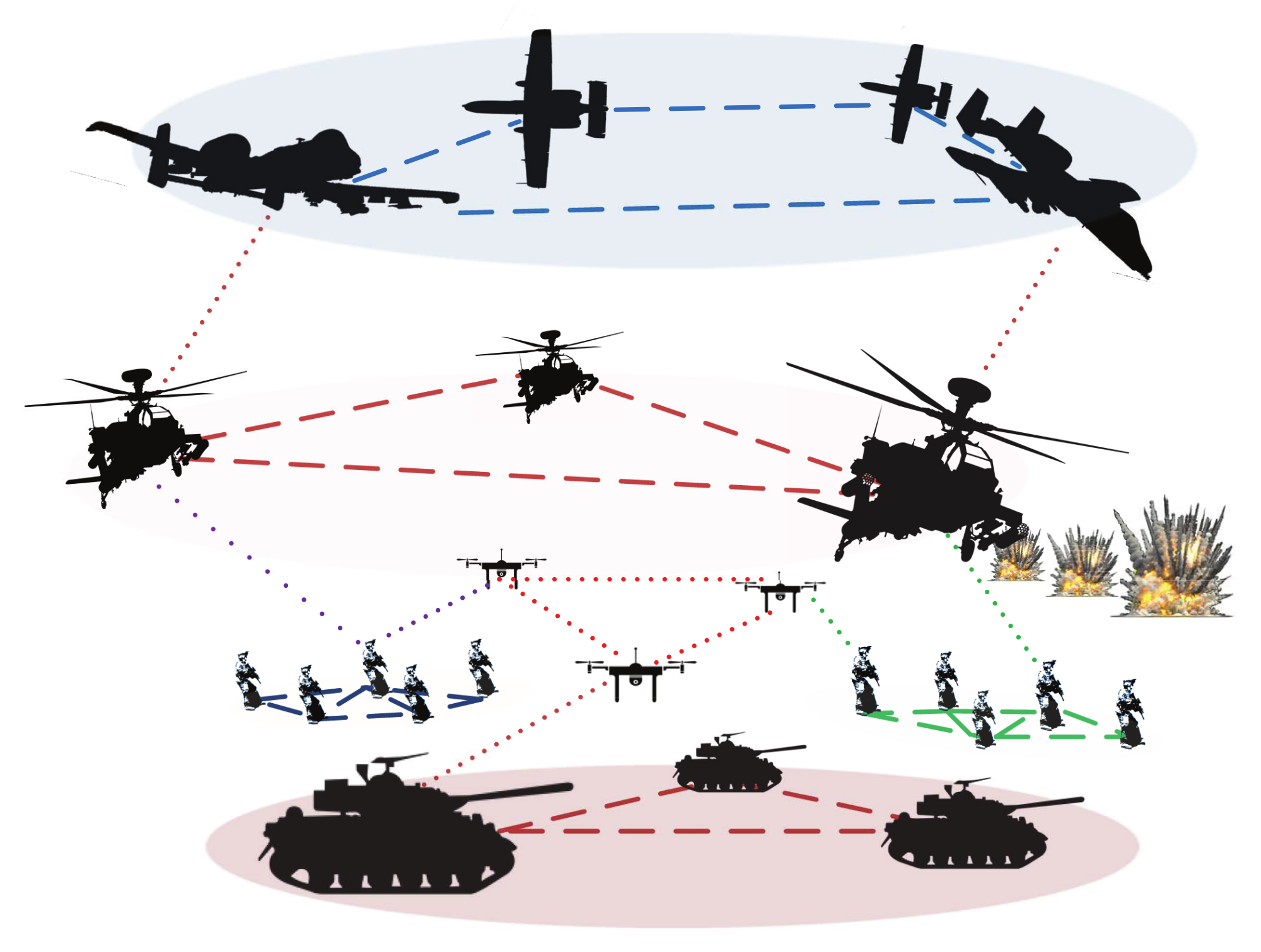Figure 1 illustrates such a network, where we can see a layer of soldiers, a layer comprised by helicopters, the intralayer links connecting “nodes” of the same layer, and interlayer links connecting “nodes” belonging to different layers.

Apparently, the requirement of calculating a CDS with minimum cardinality stems from scalability issues [3]. Additionally, from the discussion in Section 1 and in ([3] Section III.B), where “…resilience and latency requirements for synthesizing a near-optimal network” [3] are emphasized, we conclude that the more nodes with many interlayer links are included in our IoBT backbone the better it is. The inclusion of many nodes with “a lot” of interlayer links supports low-latency communication among layers; we can consider them as the hubs encountered in the literature on complex networks that reduce the “degrees of separation”. Moreover, the existence within the backbone of many nodes with “a lot” of interlayer links, reduces the danger of partitioning among layers. Therefore, we provide Definition 1 for the problem of calculating a MCDS for IoBT networks, and establish its computational complexity (Proposition 1) in the centralized setting, closing a gap in the literature which is open since [5] and it was not dealt with in [23].

Definition 1

(Multilayer MCDS problem for IoBT). Solve the $MCDS$ for a multilayer graph in a distributed manner, i.e., calculate the set $MCD{S}^{ML}$ comprised by the minimum number of nodes with the following properties: (a) their induced subgraph is connected (with intra and/or inter-layer links) and the rest of the nodes are adjacent to one node (or more) belonging to $MCD{S}^{ML}$, (b) maximize the number of dominators with many interlayer links, (c) knowing only the k-hop neighborhood of each node; we work with $k=2$ here. (Working with broader neighborhoods (i.e., $k>2$) would cause a severe broadcast storm problem [24] in order to acquire the topology deploying successive rounds of “beacon” messages).

In the rest of this section, we will investigate and establish the computational complexity of the centralized version of our problem for connected dominating sets. In particular, we will define the decision and optimization version of the examined problem, and then establish their complexities. The validity of these results for the case of connected dominating sets calculated in a distributed fashion is straightforward.

MULTILAYER CONNECTED DOMINATING SET PROBLEM

INSTANCE: A positive integer K, and a multilayer network consisting of n layers, i.e., a set of n pairs $(G_i,E_i)$, where $G_i$ is the node set of a usual network and $E_i$ is a set of edges, for $1\le i\le n$, and a set of interlayer links $E^{ML}=\{E_{i,j}\subseteq G_i\times G_j;i,j\in \{1,\cdots ,n\},i\ne j\}$.

QUESTION: Is there a dominating set of size K for $(G^{ML},E^{ML})$, i.e., a subset $V^{\prime }\subseteq (\cup V_i)$ with $|V^{\prime }|=K$ such that for all $u\in (\cup V_i)-V^{\prime }$ there is some $v_j\in (\cup V_i)$ for which $(u,v_j)\in ((\cup E_i)\cup E^{ML})$, and moreover the induced subgraph defined by $V^{\prime }$ is connected?

MULTILAYER MINIMUM CONNECTED DOMINATING SET PROBLEM

INSTANCE: A multilayer network consisting of n layers, i.e., a set of n pairs $(G_i,E_i)$, where $G_i$ is the node set of a usual network and $E_i$ is a set of edges, for $1\le i\le n$, and a set of interlayer links $E^{ML}=\{E_{i,j}\subseteq G_i\times G_j;i,j\in \{1,\cdots ,n\},i\ne j\}$.

QUESTION: What is the minimum cardinality dominating set for $(G^{ML},E^{ML})$, i.e., what is the minimum cardinality subset $V^{\prime }\subseteq (\cup V_i)$ such that for all $u\in (\cup V_i)-V^{\prime }$ there is some $v_j\in (\cup V_i)$ for which $(u,v_j)\in ((\cup E_i)\cup E^{ML})$, and moreover the induced subgraph defined by $V^{\prime }$ is connected?

We can now proceed to establish the computational complexity of the second problem. Our proof method will also establish the complexity of the first problem as well. The result is described in Proposition 1, but firstly we remind some background on proving the computational complexity of problems. So, a problem is NP-complete if the following two conditions hold:

(a)

we can prove that the problem belongs to the class of NP problems, and

(b)

we can

(b1)

either transform in polynomial-time a known NP-complete problem to the problem at hand ([25] p. 45), or

(b2)

prove that the problem at hand contains a known NP-complete problem as a special case ([25] p. 63, Section 3.2.1); this is called the “restriction” approach to proving NP-completeness.

We will now construct the proof that the problem of finding a minimum connected dominating set for $(V,E_i)$ is NP-complete. Recall that our problem is an optimization problem, i.e., “…finding the minimum dominating set”.

Proposition 1.

The Multilayer MDS problem is NP-complete.

Proof. 

Our proof consists of three steps: (a) Transform the problem into a decision version, (b) Prove that it belongs to the class of NP problems. (c) Establish its NP-completeness complexity by following the “restriction” approach, i.e., by showing that our problem contains a known NP-complete problem as a special case.

[STEP 1. Transform our optimization problem into the decision version of the same problem.]

Without violating the validity of the proof, we will work with the decision version of the problem:

Given an integer $k>0$, does our multilayer network contain a connected dominating set of cardinality equal to k?

Apparently, the smallest k for which the answer to the above problem is ‘yes’ is the size of the minimum connected dominating set of our multilayer network.

From the perspective of computational complexity, the two problems are equivalent (see item (b1) above): With the use of binary search, we need to solve the decision version for $O\left(log\right(|{\cup }_i{G}^i\left|\right))$ different values of k, i.e., which is a polynomial time of searches.

[STEP 2. Proving that the decision problem belongs to the NP class.]

The MULTILAYER CONNECTED DOMINATING SET PROBLEM is clearly in NP, as given a graph $(G^{ML},E^{ML})$, a set $S\subseteq {\cup }_i{G}^i$ of nodes, and a number k, we can test if S is a connected dominating set of $(G^{ML},E^{ML})$ of size k or less by first checking if its cardinality is less than or equal to k and then checking if every node in $(G^{ML},E^{ML})$ is either in S or adjacent to a node in S. This process clearly takes polynomial time, i.e., $O\left(\right|{\cup }_i{G}^i|+|{\cup }_i{E}^i|+|E^{ML}\left|\right)$. Should we wish to check whether S is actually connected, we can resort to any polynomial-time algorithm, e.g., breadth/depth first search. Therefore, the MULTILAYER CONNECTED DOMINATING SET PROBLEM is indeed in NP.

[STEP 3. Proving that the decision problem contains a known NP-complete problem as a special case.]

The third step of our proof involves proving that the MULTILAYER CONNECTED DOMINATING SET PROBLEM contains as a special case the problem of finding a connected dominating set for a single layer graph $G(V,E)$—a known NP-complete problem ([25] p. 190, Problem GT2).

We state the following corollary:

Corollary 1.

From ([5] Theorem 1), it follows immediately that if we wish to connect with each other two connected dominating sets of two separate graphs by adding a single edge among the two graphs, then we will need at most 2 more nodes (one from each separate graph) to be included in the single “united” connected dominating set.

We assume the existence of a single layer graph $G(V,E)$, and we construct a multilayer graph $(G^{ML},E^{ML})$ with two layers, where $G^{ML}=\{G^1,G^2\}=\{(V,E),(V,E)\}$ and $E^{ML}$ is any non-empty set of interlayer edges between $G^1$ and $G^2$. Then, we erase all but one interlayer edges from $E^{ML}$. We assume that this edge is the $(\alpha ,\beta )$ with $\alpha \in G^1$ and $\beta \in G^2$.

Then, the problem of finding whether the graph $(G^{ML},E^{ML})$ contains a connected dominating set of size $2k+\left|\right\{\alpha ,\beta \left\}\right|=2k+2$ is in an obvious one-to-one correspondence with the problem of finding whether the graph $G(V,E)$ contains a connected dominating set of size $k+1$. Note here, that there is no need—from the computational complexity perspective—for the size-$2k+2$ connected dominating set of $(G^{ML},E^{ML})$ to be a double-size clone of the size-$k+1$ connected dominating set of $G(V,E)$, and thus the two problems do not need to be an exact duplicate of each other.

Thus, the MULTILAYER CONNECTED DOMINATING SET problem is NP-complete.    □

3. Proposed Heuristic Distributed Algorithms

3.1. Distributed $CDS$ in a Multilayer Network

The calculation of a $MCDS$ by any heuristic algorithm means in practice that we are seeking for “strategically” positioned nodes in the network topology having many connections in order to decrease the size of the obtained $CDS$. In the case of IoBT networks, we seek for such nodes but with the additional property that they should have many interlayer links. So, the use of the $clPCI$centrality measure [5] is a perfect fit. We exploit $clPCI$ and incorporate it into a distributed algorithm for calculating a $CDS$; we name this distributed algorithm as the Cross layer Connected Dominating Set algorithm ($CCDS$). CCDS is composed by the CDS construction task, and the redundant relay node pruning task. As it is common in almost any distributed algorithm for wireless ad hoc networks, each node learns the topology of its neighborhood with the exchange of beacon messages. In $CCDS$, each node learns its 2-hop neighborhood $N^2\left(u\right)$; then, it calculates its clPCI and broadcasts it to its neighbours and, by mutuality of the distributed algorithm, it becomes aware of its neighbors’ clPCI values.

The initial $CDS$ construction task is a source-initiated relay node selection type of algorithm, and is divided into the neighbor prioritization subtask and the construction subtask. Each node u prioritizes (i.e., sorts) its 1-hop neighbors in decreasing order of their $clPCI$ values and progressively selects from this sorted list neighbors to include in its relay set $R\left(u\right)$ those neighbors that have the largest $clPCI$ value and that cover at least one new node in the respective 2-hop neighborhood $N^2\left(u\right)$, until all $N^2\left(u\right)$ is covered. Then, the pruning task follows, in order to reduce (if possible) the size of its relay set $R\left(u\right)$. $CCDS$ uses the restricted pruning Rule k because it is more efficient in reducing the relay node set than several existing schemes that still ensure full broadcast coverage. Differently from this scheme, we exploit connectivity information as this is quantified by $clPCI$ in order to establish a total order among nodes that participate in the $CDS$. CCDS’s pseudo-code is Algorithm 1.

Algorithm 1: CCDS

3.2. Centralized $CDS$ in Multilayer Networks

The centralized $FAST\text{-}CMDSM$ algorithm consists of the MDS discovery task, the CDS construction task, and the redundant DS node pruning task. The calculation the minimum dominating set (MDS) is treated as an Integer Programming problem [20]. The $CDS$ construction task aims at adding in the $DS$ the least possible—per node—number of nodes, such that the 2-hop neighborhood of each node is covered, and as result the multilayer network is connected in the sense that any pair of nodes can communicate via the DS. In the last task, we remove any redundant DS nodes by seeking alternative paths, and we substitute information flow via these paths. $FAST\text{-}CMDSM$’s pseudo-code is Algorithm 2.

Algorithm 2: FAST-CMDSM

3.3. Computation and Communication Complexities

3.3.1. Complexities of $CCDS$

$CCDS$ requires 7 rounds of communication among nodes to complete. In each round, at most one packet is sent over the wireless channel.

• The 2-hop neighborhood information used by the relay node set election process is collected via two rounds of information exchanges.
• In round 1, each node advertises its ID and builds its 1-hop neighbor set based on the advertisement of its neighbors.
• In round 2, each node advertises its 1-hop neighbor set and identifies links among 1-hop neighbors.
• In round 3, each node calculates its clPCI index value and advertises it together with its 2-hop neighbor set. Then, it identifies links among 2-hop neighbors.
• In round 4, each node calculates and advertises its own relay node set and updates 1-hop neighbor status.
• In round 5, the restricted Rule-k is applied to each relay node and each one of them advertises its status.
• In round 6, each node advertises its updated relay node set
• In round 7, the composition of the updated relay node set is advertised (if needed).

The computation complexity of its comprising parts is: $O\left({\Delta }^2\right)$ for the $clPCI$ calculation, and $O\left({\Delta }^3\right)$ for the relay node set election process and for the pruning phase, where $\Delta$ is the maximum node degree found in the network.

3.3.2. Complexities of $FAST\text{-}CMDSM$

$FAST\text{-}CMDSM$ is a centralized algorithm and so its communication complexity is not an issue for investigation.

$FAST\text{-}CMDSM$’ s computation complexity is exponential, similar to all branch-and-cut integer programming solvers.

4. Performance Evaluation

Competing Algorithms. We compare the proposed algorithms, namely $CCDS$ and $FAST\text{-}CMDSM$, but in order to explain the usefulness of their pruning procedures, we develop and include in our comparison their annotated with an asterisk version of them, namely $CCD{S}^{*}$ and $FAST\text{-}CMDS{M}^{*}$; these versions are simply the same algorithms but without activating the pruning procedure. Solely for illustrative purposes we include the experimentation, and $FAST\text{-}MDSM$ algorithm which constructs minimum but unconnected $DS$; we proved in [5] that any (unconnected) $DS$ of size $\parallel DS\parallel$ can be turned into a $CDS$ by adding $2\times \parallel DS\parallel$ additional nodes in the $DS$ in the worst case.

Table 1. Competitor characteristics.

	CDS	Pruning	Complexities
Competitor	Calculation	Heuristic	CPU a / Comm b
$CCDS$	Distributed	✓	${\Delta }^3$    /    7
$CCD{S}^{*}$	Distributed	-	${\Delta }^3$    /    7
$FAST\text{-}CMDSM$	Centralized	✓	${}^{exp}$    /    ${}^c$
$FAST\text{-}CMDS{M}^{*}$	Centralized	-	${}^{exp}$    /    ${}^c$
$FAST\text{-}MDSM$	Centralized	-	${}^{exp}$    /    ${}^c$

^a Δ is the maximum node degree; ^b Number of transmitted messages per node; ^c Not applicable due to its centralized nature.

summarizes the competing algorithms.

Simulation testbed. Due to the lack of available, real military networks, and the inability (The requirement of modern battlefields is to able to operate ad hoc networks consisting of an order of magnitude more nodes; for instance a battalion would need a thousand nodes. e.g., https://www.darpa.mil/news-events/2013-04-30 (accessed on 15 May 2022)) of wireless testbeds and emulation environments for ad hoc networks to deal with several hundreds of nodes, we developed a generator for multilayer networks in MATLAB. The details of our generator can be found in [6,23], and here we present its basic features. The construction of a multilayer network is driven by the average node degree, by the nodes’ number per layer (i.e., the so-called layer size), and the number of layers. The interconnection of the layers is driven by: (a) the number of a node’s links towards nodes in different layers, and (b) the distribution of the interconnections to the nodes within a particular layer. We apply the Zipfian distribution to our connectivity generator. Skewness is managed by parameter $s\in (0,1)$. We make use of four distinct Zipfian distributions, one per parameter of interest:

• $s_{degree}$: to generate the frequency of appearance of highly interconnected nodes,
• $s_{layer}$: to choose how frequently a specific layer is selected,
• $s_{node}$: to choose how frequently a specific node is selected in a specific layer.
• $s_{weight}$: to choose how uniformly the energy is distributed in the nodes.

We call these parameters as the topology skewness, and represent it as a sequence of four floats, meaning that $s_{degree}=0.5$, $s_{layer}=0.5$, $s_{node}=0.5$ and $s_{weight}=0.5$ (which are the default settings we used to create the datasets).

Performance measures. The competitors are compared in terms of the cardinality of the $CDS$; apparently an algorithm is more efficient than another, if it generates a $CDS$ having smaller cardinality [16]. Moreover, an algorithm that establishes a (per node) relay set with larger residual energy is naturally considered to be more efficient in terms of energy than another algorithm whose per node relay set has less residual energy.

Datasets. We created networks which vary with respect to the topology density, the network diameter, the number of network layers and their size. The topology density’s impact on the performance is evaluated with 4-layer networks. Each layer consists of 50 nodes, and the mean node degree is 3, or 6, or 10, or 16, or 20. The network diameter’s impact on the performance is evaluated with 4-layer networks as well. Each layer consists of 50 nodes, and the mean node degree is 6. The diameter of each layer is 3, or 5, or 8, or 12, or 17. The number of layers’ impact is examined in networks with 2, or, 3, or 4, or 5, or 7 layers. Each layer consists of 50 nodes, and the mean node degree is 6. The increase in the layer size’s impact is evaluated with 4-layer networks. The “base” layer consists of 50 nodes, and each next layer is larger than the previous by 10%, or 20%, or 30%, or 50%, or 70%. The mean node degree in each layer is 6.

Table 2. Experimentation parameters values.

Parameter	Range	Default
avg. node degree (D)	3, 6, 10, 16, 20	6
network diameter (H)	3, 5, 8, 12, 17	5
number of network layers (L)	2, 3, 4, 5, 7	4
size of a layer relative to its adjacent layers	10%, 20%, 30%, 50%, 70%	-

records all the independent parameters.

4.1. Experimental Evaluation

Each experiment was repeated 5 times. The variation around the mean was so negligible that the error bars are hardly recognizable in the plots. We conduct experiments with $s_{degree}$, $s_{layer}$, $s_{node}$, $s_{weight}$ parameters into $0.5-0.5-0.5-0.5$ (Medium skewness), and $0.1-0.1-0.1-0.1$ (Low skewness), and $0.9-0.9-0.9-0.9$ (High skewness) setting, respectively.

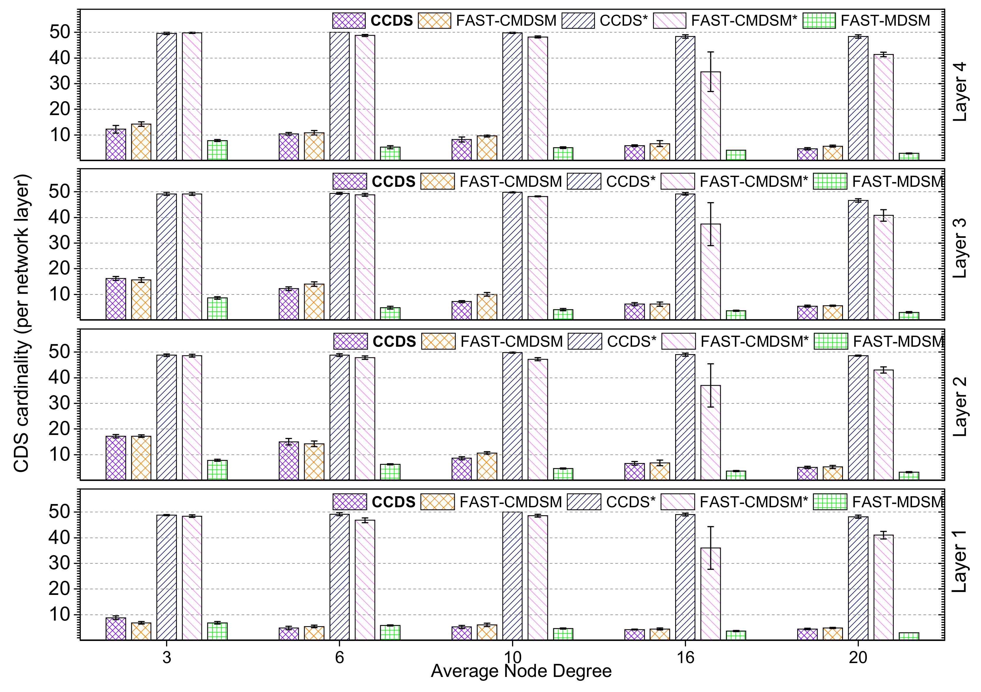
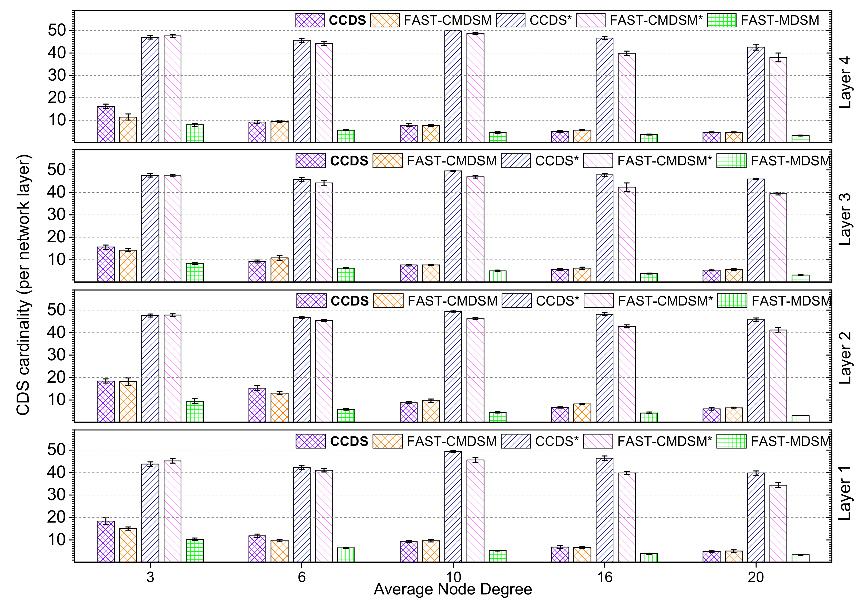
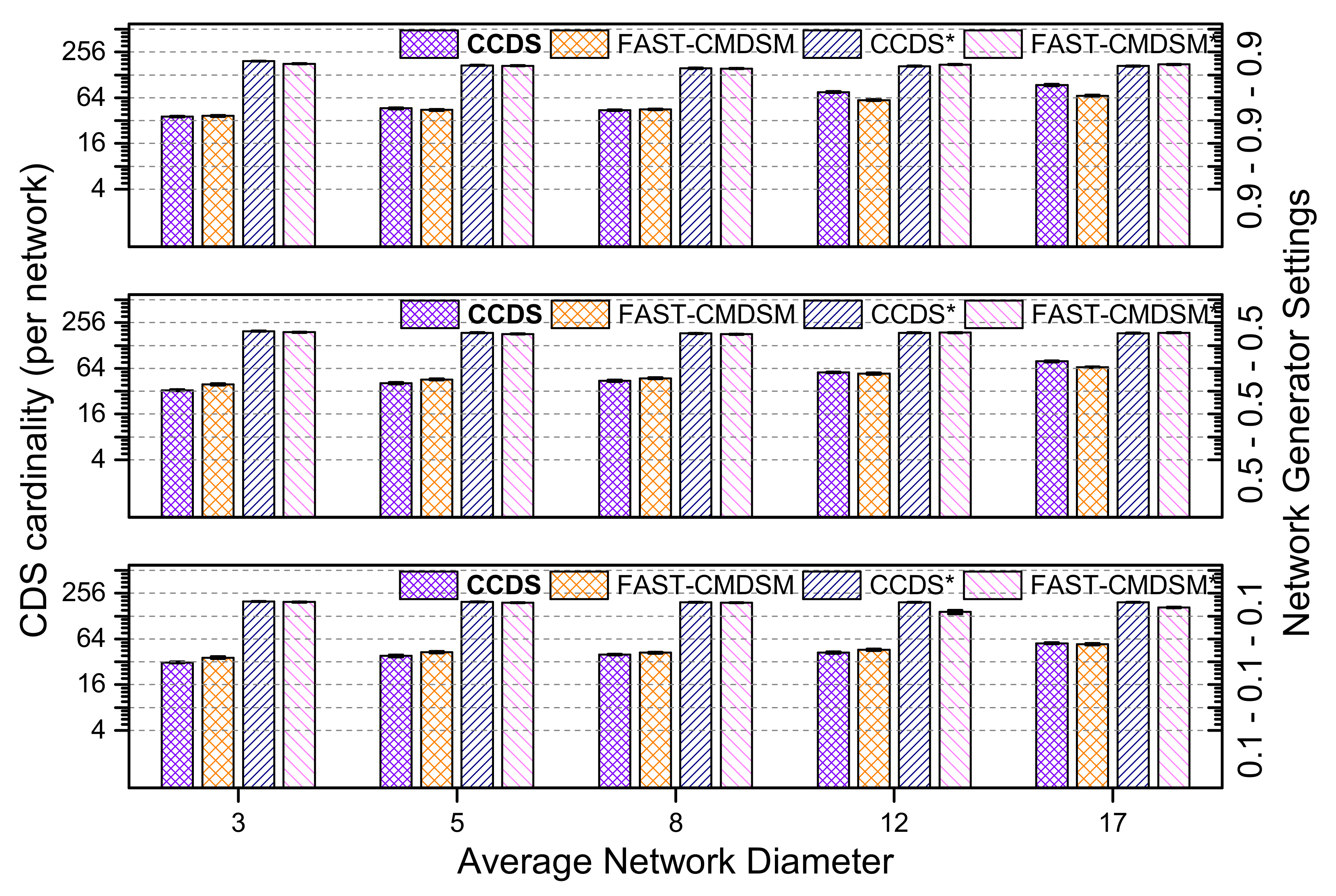
4.1.1. Impact of Topology Density

Firstly, we consider the impact of topology density on the performance of each competitor. In Figure 2 we evaluate, for medium skewness, the per layer size of the $CDS$. The main conclusion is that the size of the CDS is practically a decreasing function of the node density. This happens because the higher the network density is, the greater the coverage capability of the network nodes becomes, and therefore the size of the $CDS$ gets smaller. In the case we succeed medium skewness, there is no clear winner between $CCDS$ and $FAST\text{-}CMDSM$ as the topology becomes denser (degree ≥ 6) and both competitors present similar performance (<10% variance). The explanation is that in such topologies, there exist multiple redundant paths towards nodes, and thus both pruning mechanisms work equally well. On the contrary, in sparse topologies (degree $=3$) $FAST\text{-}CMDSM$ is up to 15% more efficient. This is due to the fact that during the pruning process, the redundant paths are less in sparse topologies, and their discovery requires knowledge of the topology further away than 2-hops, which is beyond the capabilities of localized algorithms deployed in wireless ad hoc networks. Apparently, the centralized nature of $FAST\text{-}CMDSM$ provides a clear advantage, since its pruning task has a broader overview of the topology. If we exclude the pruning task, then $CCD{S}^{*}$ and $FAST\text{-}CMDS{M}^{*}$ present similar performance (less than 10% variance) when degree ≤10, and the performance of the latter is up to 15% better to the former when degree >10. However, these results are not good news, because both algorithms do not perform well in terms of the—per layer—CDS size; i.e., the—per layer—$CDS$ size is up to 98% of that of the total number of nodes in that layer. This is considered natural in multilayer networks when the traditional methods are used (2-hop neighborhood coverage). $DS$ redundancy justifies the use of the pruning mechanism (up to $88\%$ and $85\%$$CDS$ size reduction for $CCDS$ and $FAST\text{-}CMDSM$, respectively, in this particular case).

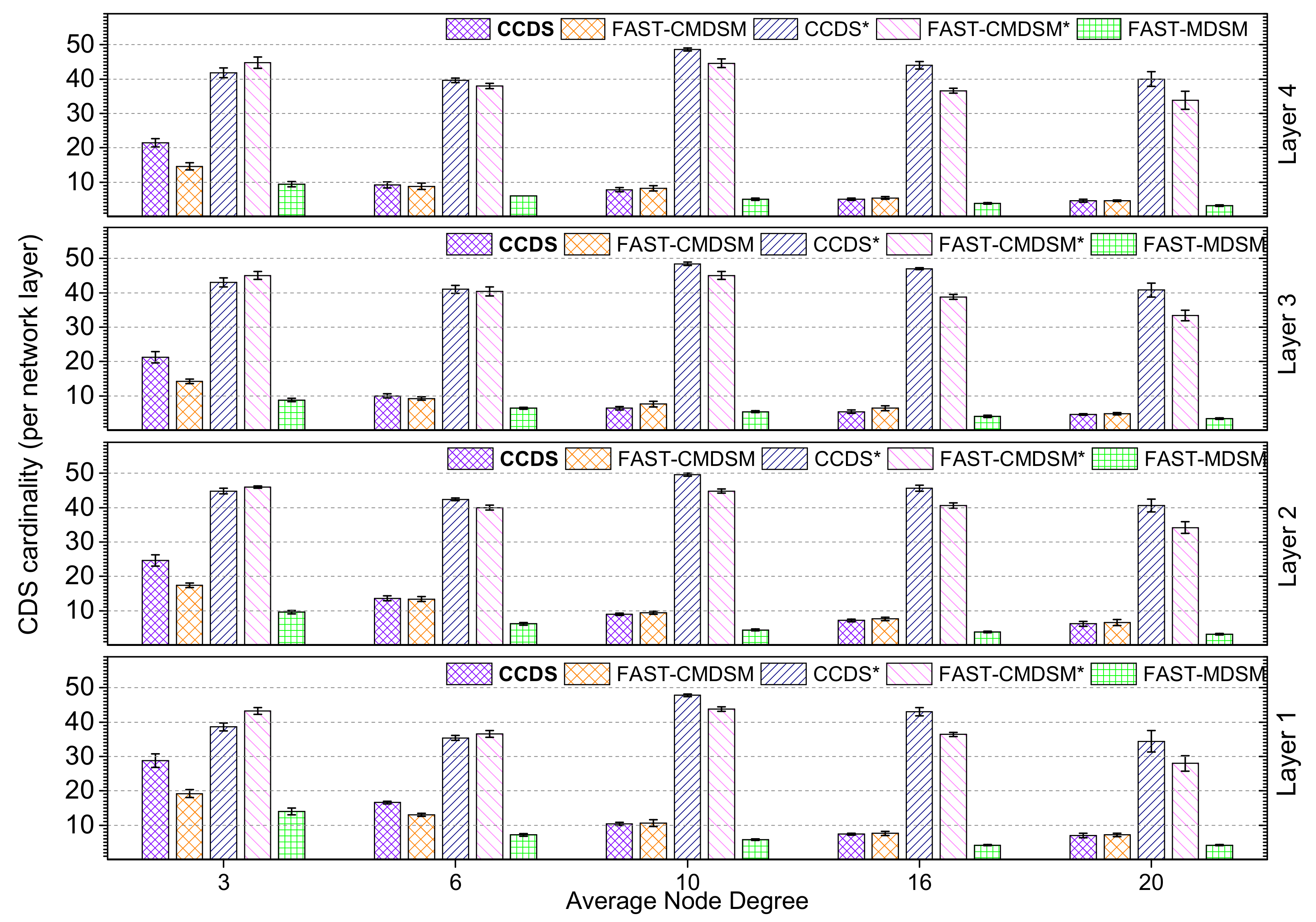
We expanded our experiments in case of low skewness. The results, depicted in Figure 3 show that there are no important differences regarding the efficiency, between $CCDS$ and $FAST\text{-}CMDSM$, when topology becomes denser (degree ≥ 6). As mentioned above, this happens because pruning mechanisms work well, when nodes have multiple ways to connect with one another. When degree = 3 (sparse topologies), $CCDS$ is about 10% less efficient than $FAST\text{-}CMDSM$, something which is justified due to the centralized control of the $FAST\text{-}CMDSM$. In this case, the reduction size of $CDS$ is about 90% for $CCDS$ algorithm and up to 88%.

In case of high skewness (see Figure 4), when degree ≥ 10, both the proposed algorithms behaves in a quite similar way (less than 10% variance), too, regarding the size of $CDS$. Here, $FAST\text{-}CMDSM$ outperforms $CCDS$, due to the centralized control of the first one which makes the procedure of finding surplus paths easier inside the Multilayer network. Examining the case when topology is sparse (degree = 3), we see that $CCDS$ is less efficient than the other pruning proposed algorithm, bearing in mind that due to the lack of enough connections, it is more difficult for a distributed algorithm to find minimum $DS$. Also, when degree = 6, $CCDS$ continues to outperform $FAST\text{-}CMDSM$, but both algorithms create $DS$ with smaller size than the above implementations do. So, in this case the efficiency of the proposed algorithms are up to 86% and up to 82% for both $CCDS$ and $FAST\text{-}CMDSM$, respectively.

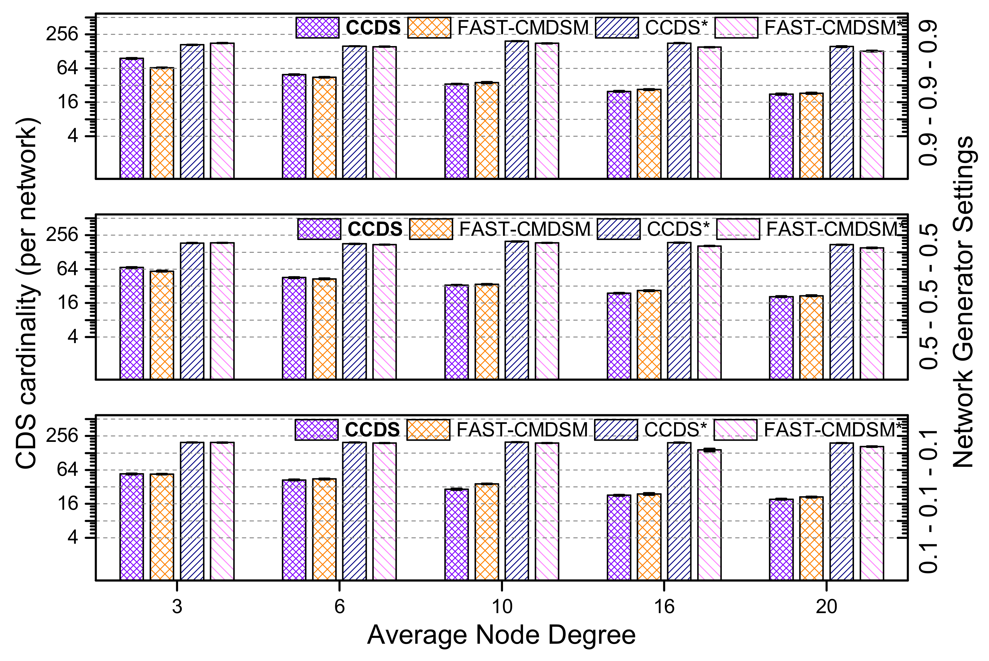
So, as it is also shown in Figure 5 which shows CDS sizes aggregated over all layers, for all the parameters tested, the results are quite similar regarding both $CCDS$ and $FAST\text{-}CMDSM$ algorithm, with the corresponding results with parameters $0.1-0.1-0.1-0.1$ to be a little more efficient, probably due to the more uniform distribution this case implements.

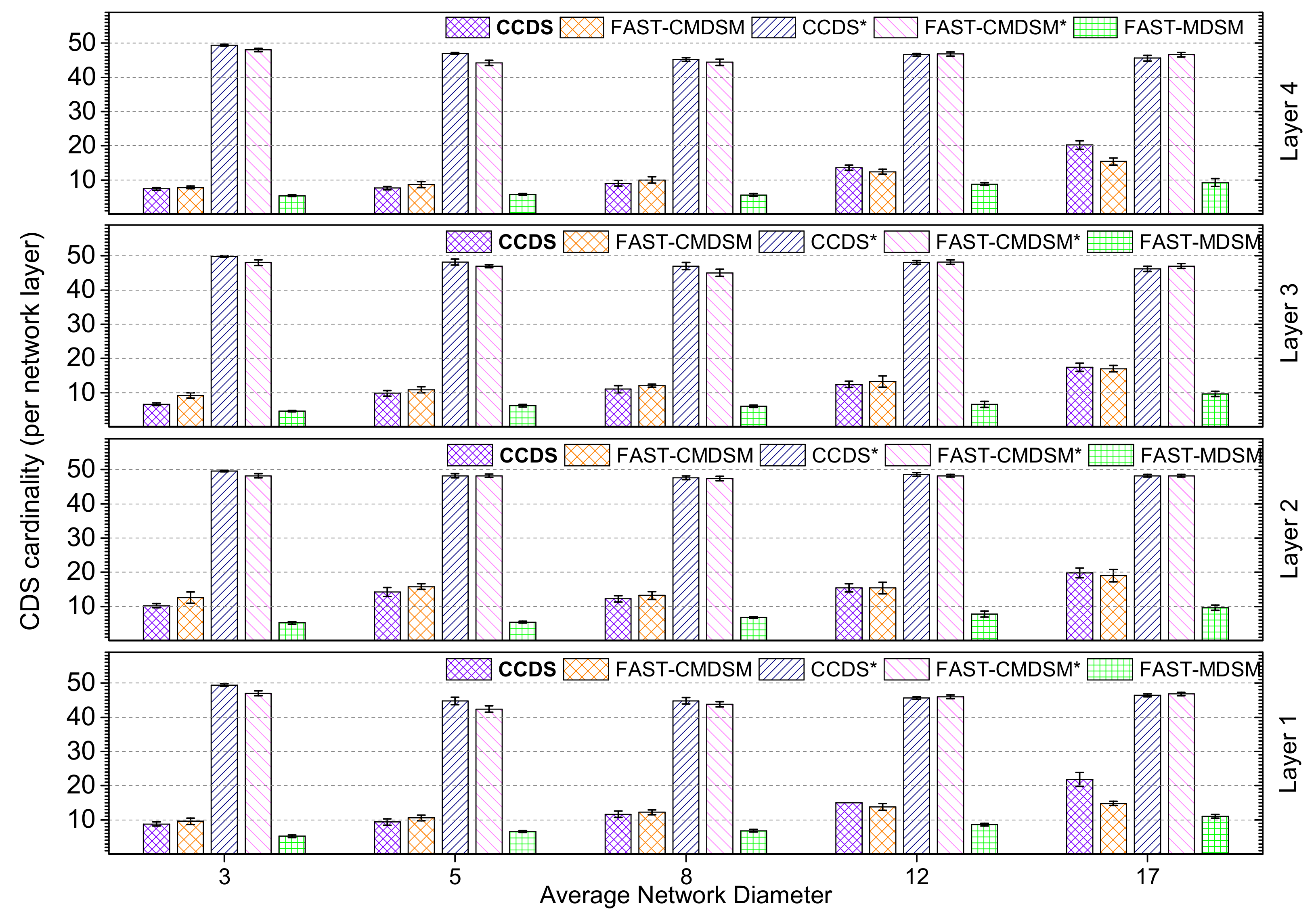
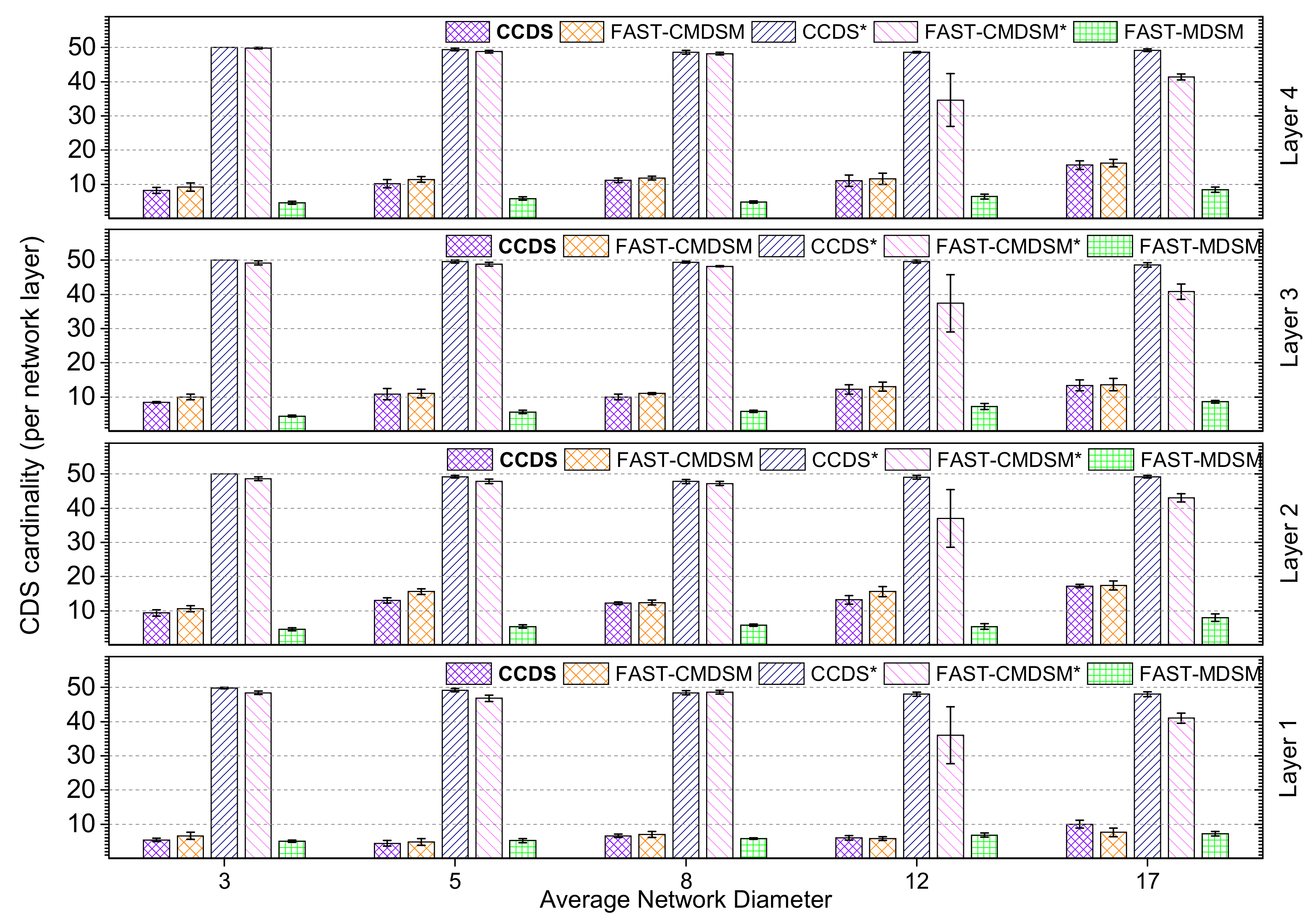
4.1.2. Impact of Network Diameter

In Figure 6, Figure 7 and Figure 8, we evaluate the effect of the network diameter in the size of the $CDS$. The main conclusion is that as the network diameter increases the size of the resulting $CDS$ increases, and this observations is valid for all competitors. In case of medium skewness (Figure 6), the diameter increases and also the topology gets sparser. So, we have fewer, longer (in hops), and less redundant paths. In that way, the selection of 1-hop neighbor nodes that cover the $N^2$ neighborhood of a particular node requires more 1-hop neighbors. Now, in terms of the competitors’ performance, we see that in bushy topologies (diameter ≤ 5) $CCDS$ presents up to $18\%$ smaller $CDS$ compared to $FAST\text{-}CMDSM$. This gain is attributed to the employment of the $clPCI$ by $CCDS$ and which helps in getting a better pruning. On the other hand, in bushy topologies an unfortunate erase from the $CDS$ of a strategically located $DS$ node will probably result in keeping a lot of (practically “useless”) $DS$ nodes just to ensure connectivity. When diameter $=8$ or diameter $=12$ the competitors have similar performance (less than 10% variance). As expected, in long and skinny topologies (diameter $=17$) $FAST\text{-}CMDSM$ outperforms $CCDS$ by $16\%$, due to its centralized nature. Examining the pruning-free versions of the competitors, we see that both of them practically exhibit the worst-case behaviour, i.e., almost all nodes are selected as $DS$ nodes; the performance of the pruning mechanism for $CCDS$ and $FAST\text{-}CMDSM$ regarding the $CDS$ size reduction is up to $83\%$ and $79\%$, respectively.

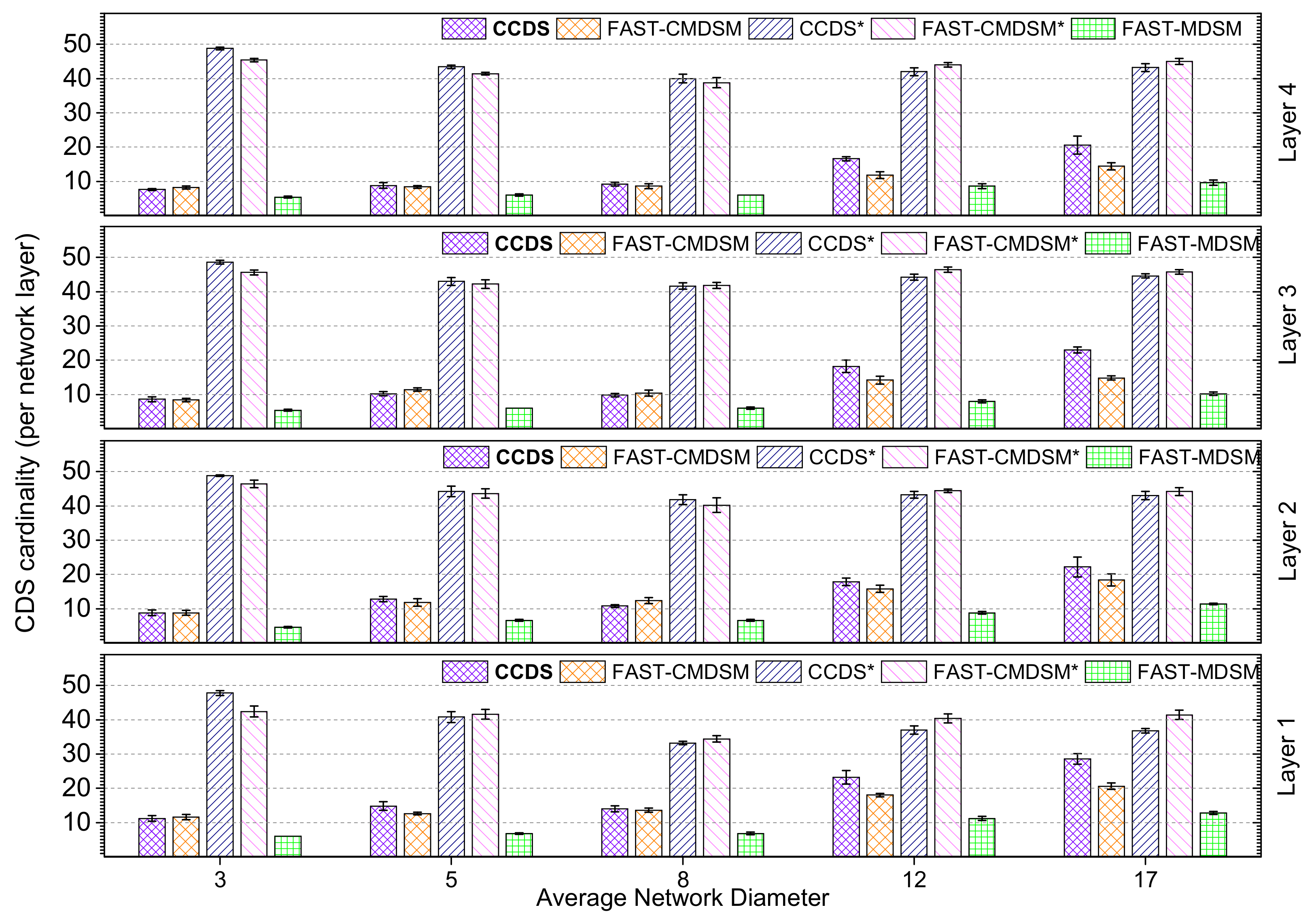
In case of low skewness as it is illustrated in Figure 7, we can also say that when diameter ≤ 5, $CCDS$ algorithm outperforms FAST-CMDSM and when diameter $=8$ or diameter $=12$, both proposed algorithms have similar performance (less than 10% variance). Finally, we see that for diameter = 17, $FAST\text{-}CMDSM$ has a better performance than $CCDS$, due to the benefits of its centralized form, in long paths. So, in this case, $CDS$ reduction is up to 85% for $CCDS$ and 81% for $FAST\text{-}CMDSM$.

Finally, when the interconnectivity generator parameters are $0.9-0.9-0.9-0.9$ (high skewness), as it is depicted in Figure 8, we observe a general increase in $CDS$ size, due to the fact that the degrees of the nodes have a great variance in this case and as a result, more nodes needed to join the $DS$. When diameter $=3$, $CCDS$ has better performance than the other proposed algorithm, due to the fact that we have smaller paths to check and as a result the distributed algorithm can discover easier the redundant paths (2-hop coverage). When diameter $=5$, or diameter $=8$, $FAST\text{-}CMDSM$ starts to have a better performance, as it creates $CDS$ with smaller size. This is expected, since the centralized control of this algorithm contributes efficiently in finding the redundant paths. The longer the diameter is, the better performance $FAST\text{-}CMDSM$ has as it is shown in Figure 8. To sum up, in this case, $CCDS$ can achieve up to 81% reduction in the size of total $CDS$, while $FAST\text{-}CMDSM$ can achieve 79%. As a summary, we provide Figure 9 to show average performance of the competitors.

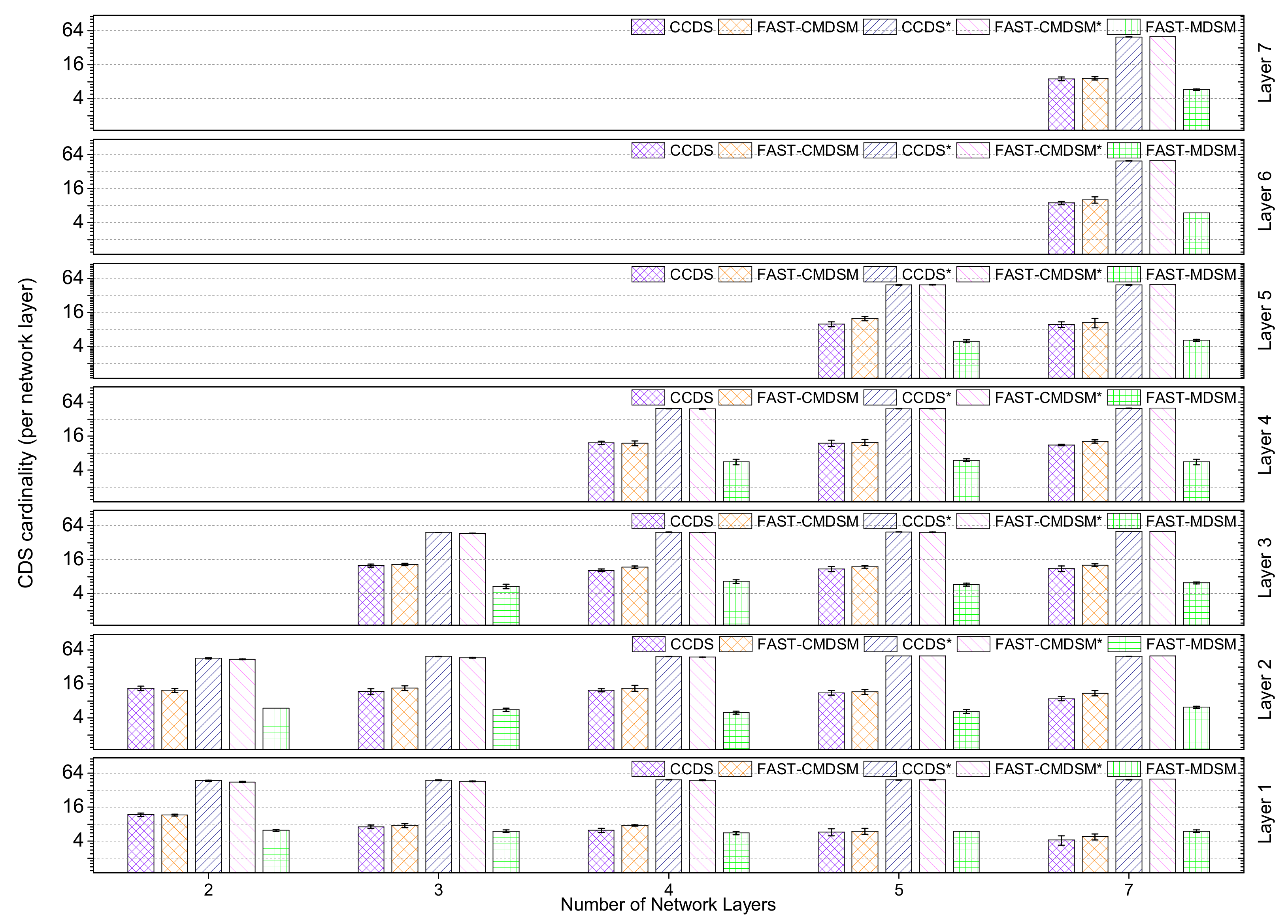
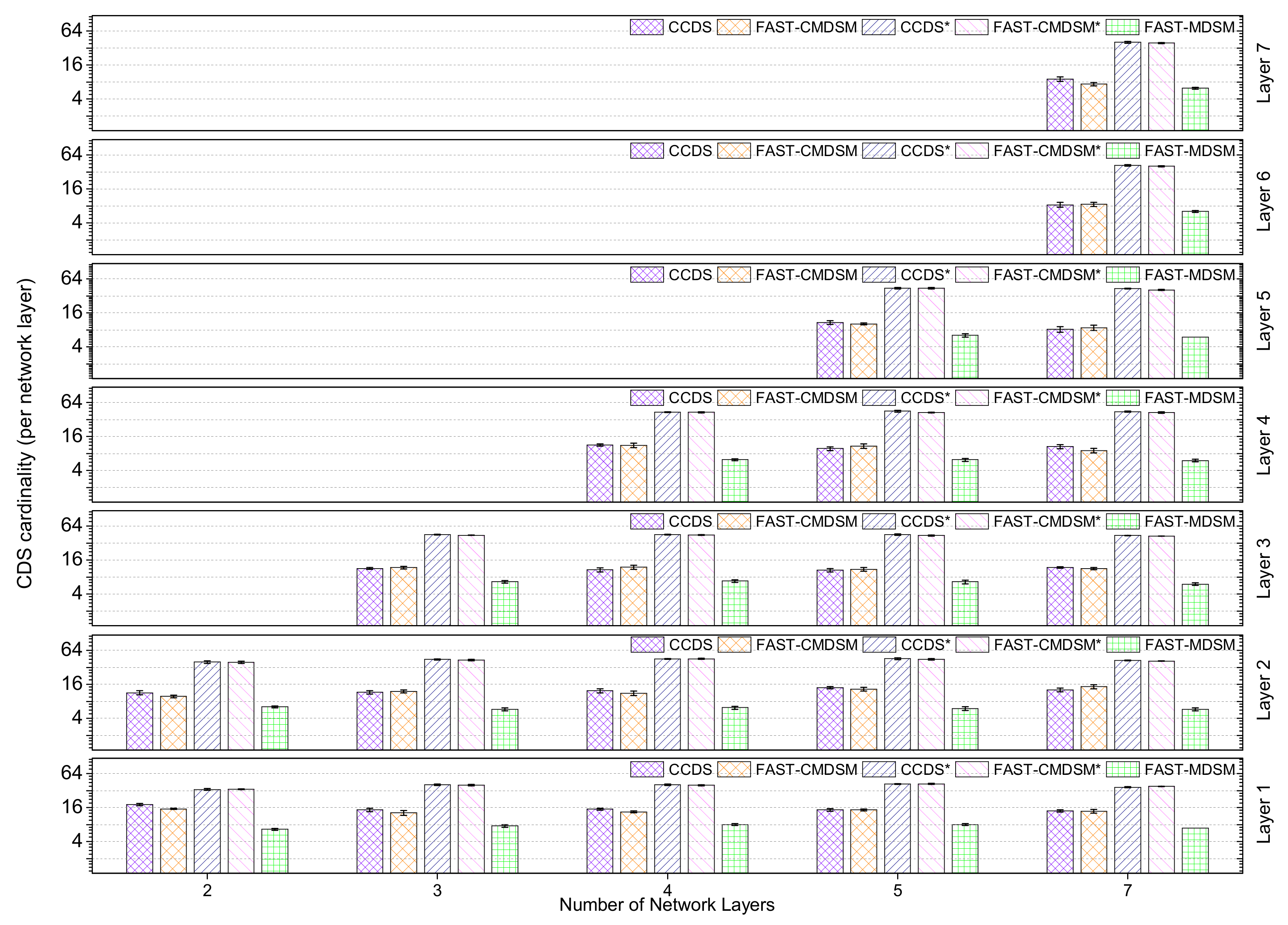
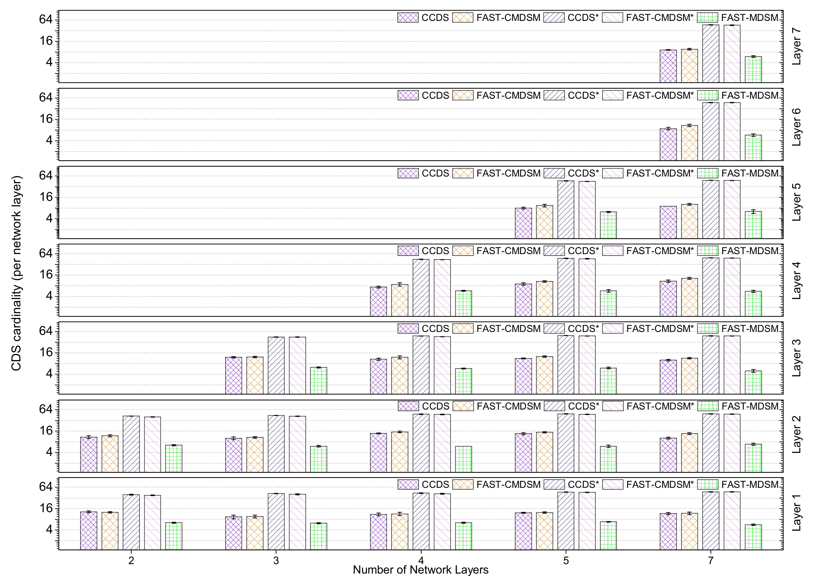
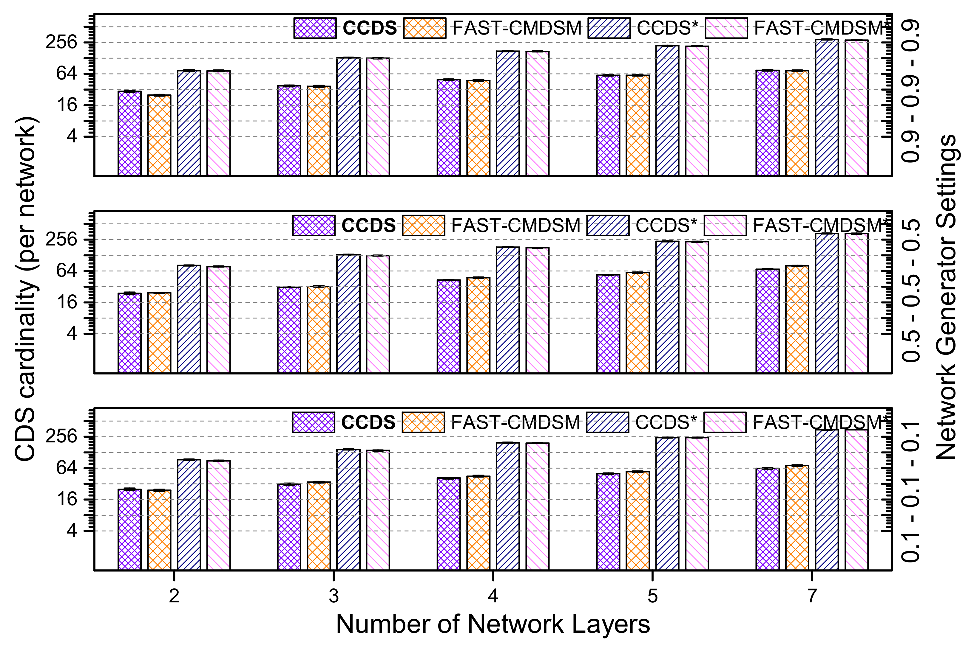
4.1.3. Impact of the Number of Layers

We investigated the impact of the network layers’ number on the competitors. In Figure 10 we show the per layer CDS cardinality for the competing algorithms (for medium skewness). The first observation we make is somewhat counter-intuitive: we see that the per layer CDS cardinality is independent on the number of layers(!) even though we would expect to be a decreasing function of the number of layers, because when a multilayer network has more layers, then it will (most probably) have more connections among layers (i.e., interlayer links), and thus the network will become more dense. So, even though we expected an increase in the coverage capability of the nodes, this does not happen, and it is attributed to the generic topology of the network. Turning now our focus on the competitors, we observe that with 5 or less layers both $CCDS$ and FAST-CMDSM perform very good (10% or less variance). However, $CCDS$ is the best of the two presenting a $14\%$ better performance. Overall, the obtained results are consistent with our earlier which state that both competitors perform very good in dense networks. In general, the main reason for CCDS’ superior performance with respect to FAST-CMDSM’ s performance is the very effective pruning mechanism. When looking at the version of these algorithms without the pruning mechanism, we see that as expected they perform poor; in particular the performance of the pruning mechanism for CCDS and FAST-CMDSM regarding the $CDS$ size reduction is up to $79\%$ and $75\%$, respectively.

Next, we present the case where the parameters of the interconnectivity generator are: $0.1-0.1-0.1-0.1$ (low skewness). We see in Figure 11, that both the proposed algorithms achieve similar performance, with the $CCDS$ algorithm to be a little bit more efficient (less than 10% variance). The total reduction in $CDS$ size is up to 80% for $CCDS$ and up to 78% for $FAST\text{-}CMDSM$. The last experiment in this section is conducted by setting the respective interconnectivity generator variables to: $0.9-0.9-0.9-0.9$ (high skewness). In this case, when number of layers is less than 4, $FAST\text{-}CMDSM$ outperforms $CCDS$, while when the number of layers is greater than 4, then the two proposed algorithms are barely equally efficient, as it is shown in Figure 12. Specifically, the total reduction provided by this experiment is up to 74% for CCDS and up to 73% for $FAST\text{-}CMDSM$ (1% variance). In Figure 13 we show the competitors average performance.

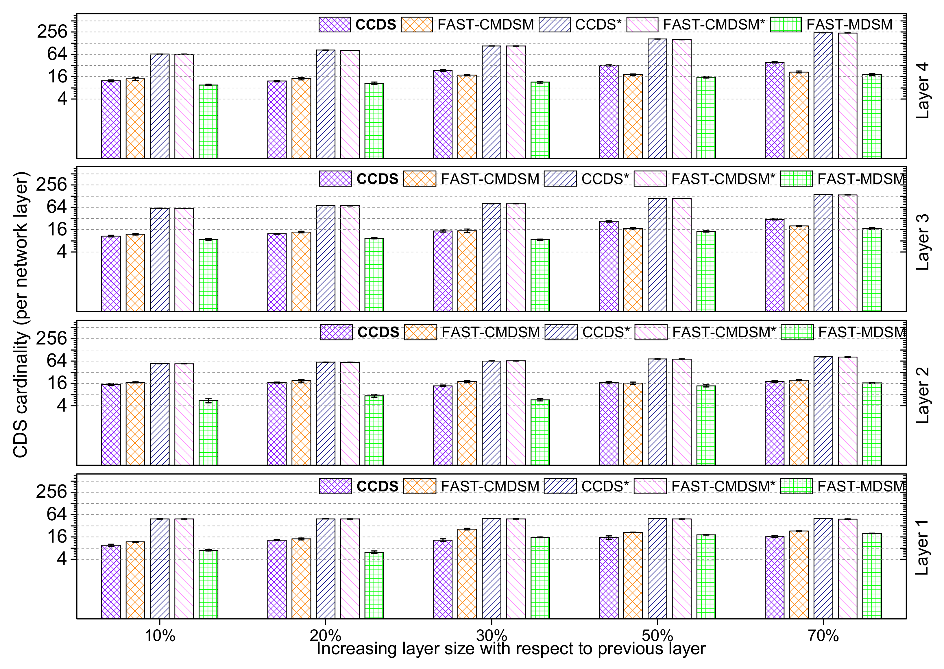
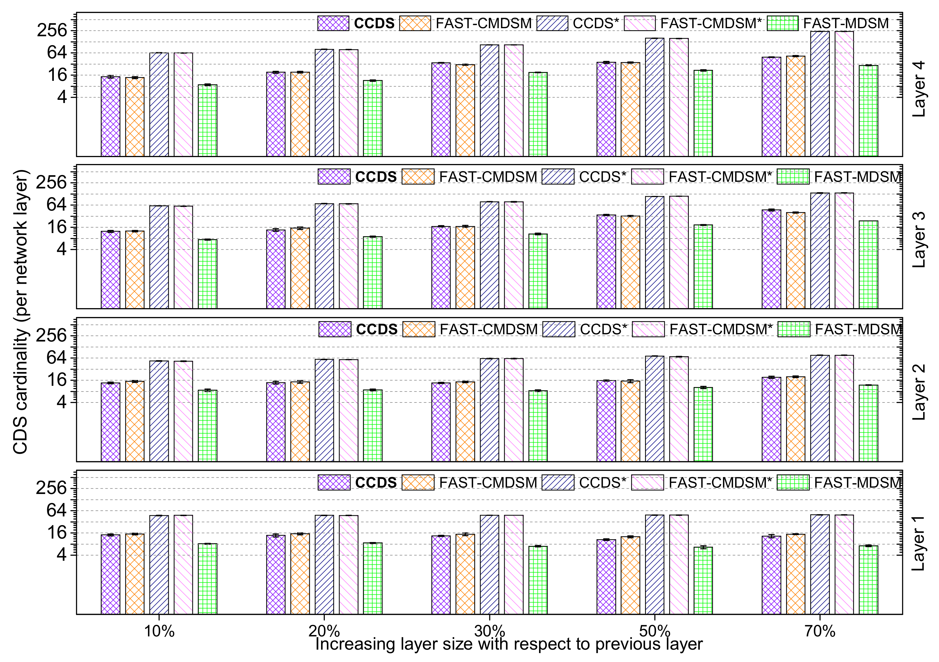
4.1.4. Impact of Layer’s Size Increase

Here we consider the impact of layer’s size increase on the competitors’ performance; we evaluate the per layer size of the $CDS$ for medium skewness, and depict the results in Figure 14. A first, generic observation is that the cardinality of CDS increases with increasing layer size. This is easily explained by the fact that the as the size of each layer increases, so does the need for more nodes to act as connectors, and consequently we get a larger CDS. Looking at the performance of the competitors, we note that an increase in the size of each subsequent layer by $30\%$ or less results in having $CCDS$ to outperform $FAST\text{-}CMDSM$ with a margin from 11% up to $16\%$. The basic reason behind that is the dense topology, with the consequence that many redundant paths remain within the vicinity of $CCDS$ (i.e., 2-hop), and therefore the pruning process eliminates many redundant dominators. On the contrary, an increase in the size of each subsequent layer by $50\%$ or more results in having the centralized $FAST\text{-}CMDSM$ outperform $CCDS$ from $18\%$ up to $21\%$. This is expected, since the large difference in the cardinality of the layers implies a large number of interlayer links, and therefore the calculation of the redundant paths by the pruning process requires a broader/global view of the topology, which is only available to the centralized FAST-CMDSM algorithm and not the distributed $CCDS$ algorithm. As a last comment to this experiment, we see that the versions without pruning of the algorithms select almost all nodes as dominators; in particular the performance of the pruning mechanism for $CCDS$ and $FAST\text{-}CMDSM$ regarding the $CDS$ size reduction is up to $80\%$ and $83\%$, respectively.

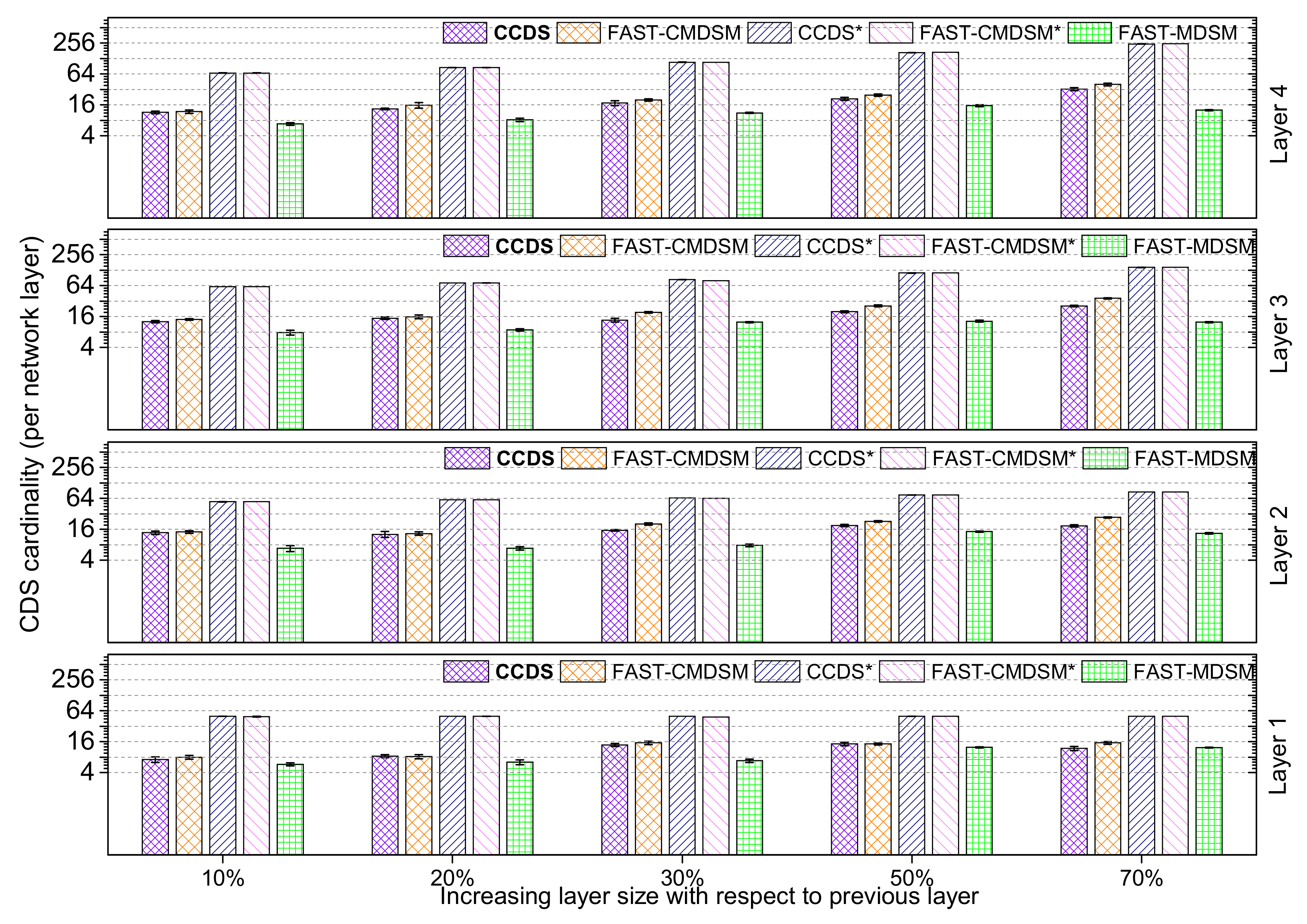
Conducting the experiment by changing the set of variables in the interconnectivity generator to $0.1-0.1-0.1-0.1$ (almost uniform distribution), we observe that $CCDS$ is the champion algorithm, because of the dense topologies formed, as it is shown in Figure 15. In this case, $CCDS$ achieves 82% reduction in the total $CDS$ size, while $FAST\text{-}CMDSM$ achieves 80%. The last experiment in this section is conducted by setting the respective interconnectivity generator parameters to: $0.9-0.9-0.9-0.9$ and the results are presented in Figure 16. In this case, we have a barely arbitrarily-formed distribution (high skewness). We see that while increasing the number of nodes, set in every layer, the $CCDS$ algorithm remains our best option, as it is justified above. In this case, $CCDS$ achieves 76% reduction in the total $CDS$ size, while $FAST\text{-}CMDSM$ achieves 75%.

Comparing the experiments, done, by changing the values in variables of skewness, we conclude that having a more uniform distribution (Low Skewness) is the best scenario, in which, our algorithms achieves their highest efficiency. This happens because this type of distribution, normalizes well the degree of every node in every layer, which means less nodes are important for the coverage of the network and this results in smaller $CDS$ size. On the other hand, when we have high skewness, nodes are arbitrarily connected which means, more nodes in total $DS$ are needed in order to cover the whole network properly. Furthermore, in every case, $CCDS$ is the more efficient algorithm to use, bearing in mind that in every section, it provides better reduction from $FAST\text{-}CMDSM$, except for the one in which we examine low skewness and our variables are set to 0.5 in which $FAST\text{-}CMDSM$ outperforms $CCDS$ (3% variance).

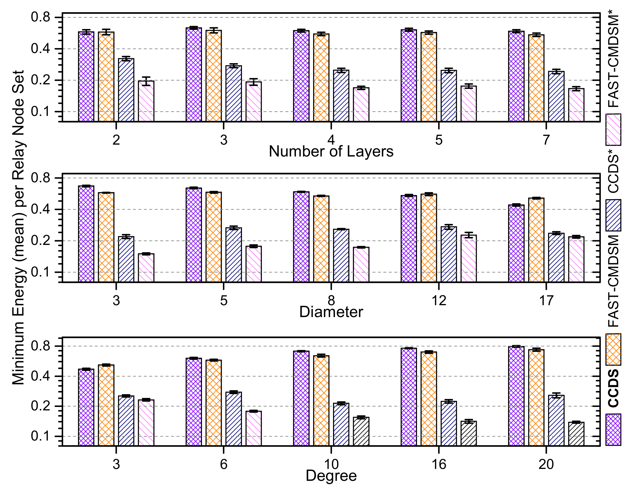
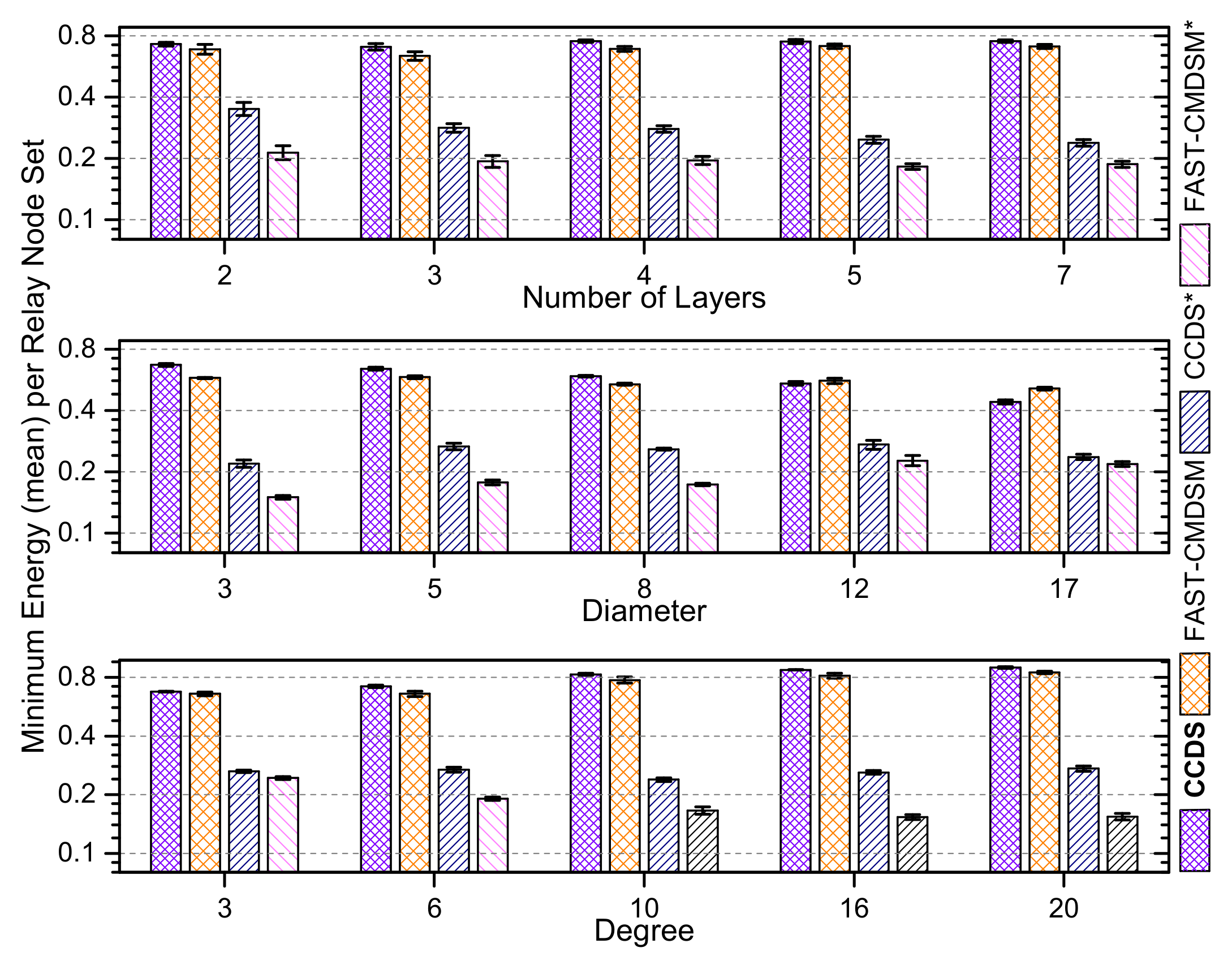
4.1.5. Energy Awareness of the Competing Algorithms

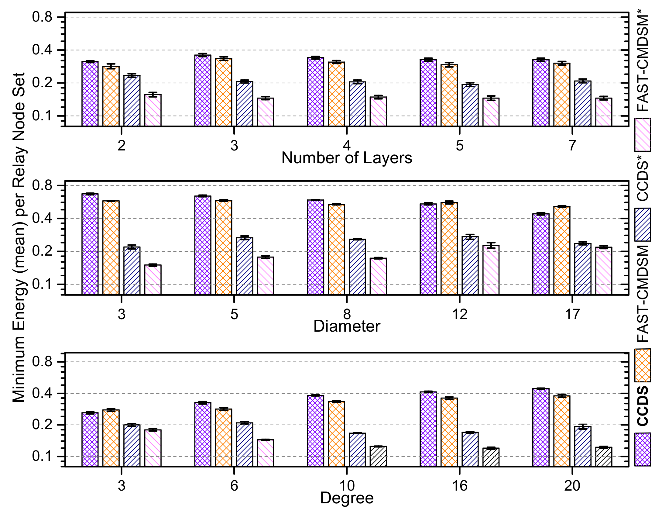
We repeated all experiments taking now into account the residual energy of each node, and we show here the obtained results which concern the aggregated over all network layers performance of the competitors. In Figure 17, we report the results for medium skewness and we see that $CCDS$ selects the most energy efficient $CDS$ in, almost, any case, followed by $FAST\text{-}CMDSM$. We end up in the same conclusion about $CCDS$ algorithm’s energy consumption regarding both the experiments of low and high skewness, as it is depicted in both Figure 18 and Figure 19, respectively.

4.1.6. Results’ Summary

In

Table 3. Results’ summary.

Parameter	Avg Performance Gain of CCDS
topology density	≈12%
network diameter	≈8.5%
number of layers	≈14%
layers’ heterogeneity	≈18%

we provide a summary of $CCDS$ average performance gain (percentage-wise) over the second best performing distributed algorithm across the independent parameter space.

5. Conclusions

The Internet of Battlefield Things is a new cyberphysical system originating from the Internet of Things, but at a much larger scale, and with stringent robustness and latency requirements. Its most significant and challenging goal is to carry out commander’s intent in a safe, responsive and resilient manner. This article investigated the issue of building small and resilient backbones for IoBT networks. We abstracted the topology of an IoBT network as a multilayer graph, and we resorted to the concept of dominating sets to achieve our goal. Then, we presented a distributed algorithm for calculating connected dominating sets with small-cardinality in this multilayer network context. We implemented and contrasted our proposed algorithm to two state-of-the-art algorithms for computing connected dominating sets for multilayer networks using generated topologies. Our algorithm showed constantly better performance against these competitors across a range of topologies with various representative features. Our future research involves algorithmic issues of detecting multiple MCDS for energy conservation via sleep-scheduling.

References

1. Kott, A.; Swami, A.; West, B.J. The Internet of Battle Things. IEEE Comput. Mag. 2016, 49, 70–75. [Google Scholar] [CrossRef]
2. Russel, S.; Abdelzaher, T. The Internet of Battlefield Things: The next generation of command, control, communications and intelligence (C3I) decision-making. In Proceedings of the 2018 IEEE Military Communications Conference (MILCOM 2018), Los Angeles, CA, USA, 29–31 October 2018; pp. 737–742. [Google Scholar]
3. Abdelzaher, T.; Ayanian, N.; Basar, T.; Diggavi, S.; Diesner, J.; Ganesan, D.; Govindan, R.; Jha, S.; Lepoint, T.; Marlin, B. Will distributed computing revolutionize peace? The emergence of Battlefield IoT. In Proceedings of the IEEE International Conference on Distributed Computing Systems, Vienna, Austria, 2–6 July 2018; pp. 1129–1138. [Google Scholar]
4. Abdelzaher, T.; Ayanian, N.; Basar, T.; Diggavi, S.; Diesner, J.; Ganesan, D.; Govindan, R.; Jha, S.; Lepoint, T.; Marlin, B.; et al. Toward and Internet of Battle Things: A resilience perspective. IEEE Comput. Mag. 2018, 51, 24–36. [Google Scholar] [CrossRef]
5. Papakostas, D.; Basaras, P.; Katsaros, D.; Tassiulas, L. Backbone formation in military multi-layer ad hoc networks using complex network concepts. In Proceedings of the IEEE Military Communications Conference, Baltimore, MD, USA, 1–3 November 2016; pp. 842–848. [Google Scholar]
6. Papakostas, D.; Eshghi, S.; Katsaros, D.; Tassiulas, L. Energy-aware backbone formation in military multilayer ad hoc networks. Ad Hoc Netw. 2018, 81, 17–44. [Google Scholar] [CrossRef]
7. Farooq, M.J.; Zhu, Q. On the secure and reconfigurable multi-layer network design for critical information dissemination in the Internet of Battlefield Things (IoBT). IEEE Trans. Wirel. Commun. 2018, 17, 2618–2632. [Google Scholar] [CrossRef]
8. Gaikwad, N.B.; Ugale, H.; Keskar, A.; Shivaprakash, N.C. The Internet-of-Battlefield-Things (IoBT)-based enemy localization using soldiers location and gunshot direction. IEEE Internet Things J. 2020, 7, 11725–11734. [Google Scholar] [CrossRef]
9. Abuzainab, N.; Saad, W. Dynamic connectivity game for adversarial Internet of Battlefield Things Systems. IEEE Internet Things J. 2018, 5, 378–390. [Google Scholar] [CrossRef] [Green Version]
10. Abuzainab, N.; Saad, W. A multiclass mean-field game for thwarting misinformation spread in the Internet of Battlefield Things. IEEE Trans. Commun. 2018, 66, 6643–6658. [Google Scholar] [CrossRef] [Green Version]
11. Azmoodeh, A.; Dehghantanha, A.; Choo, K.K.R. Robust malware detection for Internet of (Battlefield) Things devices using deep eigenspace learning. IEEE Trans. Sustain. Comput. 2019, 4, 88–95. [Google Scholar] [CrossRef]
12. Castiglione, A.; Choo, K.K.R.; Nappi, M.; Ricciardi, S. Context aware ubiquitous biometrics in edge of military things. IEEE Cloud Comput. Mag. 2017, 4, 16–20. [Google Scholar] [CrossRef]
13. Nasim, I.; Kim, S. Human EMF exposure in wearable networks for Internet of Battlefield Things. In Proceedings of the IEEE Military Communications Conference, Norfolk, VA, USA, 12–14 November 2019. [Google Scholar]
14. Stojmenovic, I.; Seddigh, M.; Zunic, J. Dominating sets and neighbor elimination-based broadcasting algorithms in wireless networks. IEEE Trans. Parallel Distrib. Syst. 2002, 13, 14–25. [Google Scholar] [CrossRef] [Green Version]
15. Wu, J.; Li, H. On calculating connected dominating set for efficient routing in ad hoc wireless networks. In Proceedings of the Workshop on Discrete Algorithms and Methods for Mobile Computing and Communications, Seattle, WA, USA, 20 August 1999; pp. 7–14. [Google Scholar]
16. Yu, J.; Wang, N.; Wang, G.; Yu, D. Connected dominating sets in wireless ad hoc and sensor networks: A comprehensive survey. Comput. Commun. 2013, 24, 121–134. [Google Scholar] [CrossRef]
17. Zhao, D.; Xiao, G.; Wang, Z.; Wang, L.; Xu, L. Minimum dominating set of multiplex networks: Definition, application, and identification. IEEE Trans. Syst. Man Cybern. Syst. 2021, 51, 7823–7837. [Google Scholar] [CrossRef]
18. Wu, Y.; Li, Y. Construction algorithms for k-connected m-dominating sets in wireless sensor networks. In Proceedings of the ACM International Symposium on Mobile Ad Hoc Networking and Computing, Hong Kong, China, 26–30 May 2008; pp. 83–90. [Google Scholar]
19. Pemmaraju, S.V.; Pirwani, I.A. Energy conservation via domatic partitions. In Proceedings of the ACM International Symposium on Mobile Ad Hoc Networking and Computing, Florence, Italy, 22–25 May 2006; pp. 143–154. [Google Scholar]
20. Nacher, J.C.; Ishitsuka, M.; Miyazaki, S.; Akutsu, T. Finding and analysing the minimum set of driver nodes required to control multilayer networks. Nat. Sci. Rep. 2019, 9, 1–12. [Google Scholar] [CrossRef] [PubMed]
21. Fan, N.; Watson, J.P. Solving the connected dominating set problem and power dominating set problem by integer programming. In Proceedings of the International Conference on Combinatorial Optimization and Applications, Banff, AB, Canada, 5–9 August 2012; pp. 371–383. [Google Scholar]
22. Haynes, T.W.; Hedetniemi, S.; Slater, P. Fundamentals of Domination in Graphs; Chapman & Hall/CRC Pure and Applied Mathematics; CRC Press: Boca Raton, FL, USA, 1998. [Google Scholar]
23. Papakostas, D.; Kasidakis, T.; Fragkou, F.; Katsaros, D. Backbones for Internet of Battlefield Things. In Proceedings of the IEEE/IFIP Annual Conference on Wireless On-Demand Network Systems and Services, Klosters, Switzerland, 9–11 March 2021; pp. 116–123. [Google Scholar]
24. Tseng, Y.C.; Ni, S.Y.; Chen, Y.S.; Sheu, J.P. The broadcast storm problem in a mobile ad hoc network. Wirel. Netw. 2002, 8, 153–167. [Google Scholar] [CrossRef]
25. Garey, M.R.; Johnson, D.S. Computers and Intractability: A Guide to the Theory of NP-Completeness; W. H. Freenan and Company: New York, NY, USA, 1979. [Google Scholar]
Figure 1. A sample multilayer IoBT ad hoc network.
Futureinternet 14 00186 g001
Figure 2. Impact of topology density (Medium skewness).
Futureinternet 14 00186 g002
Figure 3. Impact of topology density (Low skewness).
Futureinternet 14 00186 g003
Figure 4. Impact of topology density (High skewness).
Futureinternet 14 00186 g004
Figure 5. Impact of topology density (CDS size aggregated over all layers).
Futureinternet 14 00186 g005
Figure 6. Impact of network diameter (Medium skewness).
Futureinternet 14 00186 g006
Figure 7. Impact of network diameter (Low skewness).
Futureinternet 14 00186 g007
Figure 8. Impact of network diameter (High skewness).
Futureinternet 14 00186 g008
Figure 9. Impact of network diameter (CDS size aggregated over all layers).
Futureinternet 14 00186 g009
Figure 10. Impact of number of layers (Medium skewness).
Futureinternet 14 00186 g010
Figure 11. Impact of number of layers (Low skewness).
Futureinternet 14 00186 g011
Figure 12. Impact of number of layers (High skewness).
Futureinternet 14 00186 g012
Figure 13. Impact of number of layers (CDS size aggregated over all layers).
Futureinternet 14 00186 g013
Figure 14. Impact of increasing layer cardinality (Medium skewness).
Futureinternet 14 00186 g014
Figure 15. Impact of increasing layer cardinality (Low skewness).
Futureinternet 14 00186 g015
Figure 16. Impact of increasing layer cardinality (High skewness).
Futureinternet 14 00186 g016
Figure 17. Energy awareness of the competitors (Medium skewness).
Futureinternet 14 00186 g017
Figure 18. Energy awareness of the competitors (Low skewness).
Futureinternet 14 00186 g018
Figure 19. Energy awareness of the competitors (High skewness).
Futureinternet 14 00186 g019