Deep Regression Neural Networks for Proportion Judgment

Abstract

Deep regression models are widely employed to solve computer vision tasks, such as human age or pose estimation, crowd counting, object detection, etc. Another possible area of application, which to our knowledge has not been systematically explored so far, is proportion judgment. As a prerequisite for successful decision making, individuals often have to use proportion judgment strategies, with which they estimate the magnitude of one stimulus relative to another (larger) stimulus. This makes this estimation problem interesting for the application of machine learning techniques. In regard to this, we proposed various deep regression architectures, which we tested on three original datasets of very different origin and composition. This is a novel approach, as the assumption is that the model can learn the concept of proportion without explicitly counting individual objects. With comprehensive experiments, we have demonstrated the effectiveness of the proposed models which can predict proportions on real-life datasets more reliably than human experts, considering the coefficient of determination (>0.95) and the amount of errors (MAE < 2, RMSE < 3). If there is no significant number of errors in determining the ground truth, with an appropriate size of the learning dataset, an additional reduction of MAE to 0.14 can be achieved. The used datasets will be publicly available to serve as reference data sources in similar projects.

1. Introduction

People have the ability to distinguish between non-symbolic numerical magnitudes without counting, which is derived from the approximate number system (ANS) [1]. At the same time, various tasks require people to estimate ratios and proportions, comparing the magnitudes of two quantities [2]. Determining the proportion of open flowers to all the flower buds and flowers on the plant, estimating the ratio between a marked area and the total area of an image, and judging the share of a certain object in relation to the total number of objects on an image all serve as everyday examples. In this paper, we focus on the proportion judgment, where, by definition [2], an observer estimates the magnitude of one stimulus relative to another, larger stimulus, and based on that responds with a value between 0 and 1 (or between 0% and 100%). Proportion judgment can be seen as a special case of ratio judgment, where the observer estimates the ratio of two stimulus magnitudes. It should also be mentioned that, in everyday life, the terms proportion, ratio, fraction, or percentage are used interchangeably.

Although proportion estimation can be an important prerequisite for decision-making (for example, plant protection with chemical or biological products, within optimal timelines), numerous studies have shown that bias is systematically present in the assessment.

Several authors have shown that small proportions are usually overestimated, and large proportions underestimated [3,4]. Notably, there are fewer studies that discuss the reverse pattern, i.e., underestimation of small proportions and overestimation of large proportions. Therefore, the problem of proportion estimation represents a suitable area for the application of artificial intelligence (AI) techniques.

In computer vision, regression techniques can be applied in many fields, such as crowd counting, pose estimation, facial landmark detection, age and demographic analysis estimation, or image registration [5]. Nowadays, the convolutional neural network (CNN) is considered to be one of the best learning algorithms for understanding image content and has shown exemplary performance in a number of applications [6]. The common mode of implementation is deep regression, i.e., CNN with a (linear) regression top layer.

For example, the authors in [7] proposed deep regression forests for age estimation. In [8], the authors used a ResNet-based deep regression model to learn the optimal repulsive pose for the safe collaboration between humans and robots. Deep learning methods modified for regression problems [9] were also applied to estimate gross tonnage, as a nonlinear measure of a ship’s overall internal volume. Deng et al. [10] used a deep regression framework based on manifold learning for manufacturing quality prediction. In [11], authors proposed a part-to-target tracker based on a deep regression model. Zhong et al. [12] applied an attention-guided deep regression architecture for cephalometric landmark detection. Single poultry tracking is demonstrated in [13], using a deep regression architecture based on the Alexnet network.

Wang et al. [14] proposed a deep regression framework for automatic pneumonia screening, which jointly learns the multi-channel images and multi-modal information to simulate the clinical pneumonia screening process. In [15], hierarchical deep regression with a network designed for hierarchical semantic feature extraction is used for traffic congestion detection, as an important aspect of vehicular management. The authors proposed in [16] the use of a regression convolutional neural network to find the 3-D position of arbitrarily oriented subjects or anatomy in a canonical space based on slices or volumes of medical images. With these examples, it becomes clear that deep regression algorithms are used in a wide variety of applications in very different domains.

There are many different approaches to this topic, as shown by the examples of applying machine learning or other similar techniques in the field of land cover classification. Such examples include plant communities, crops, and fractional vegetation cover estimation [17,18,19,20,21,22,23]. Other areas of application are very broad; for example, these methods could be applied in geology and rock fraction estimation [24], biology [25], or medicine [26]. One of the few examples of the application of deep learning algorithms is [27], where the authors propose a model for proportion estimation for urban mixed scenes. In the proposed framework, the feature extraction capabilities of deep learning are used to obtain the fully connected layer features, after which a scene-unmixing framework based on nonnegative matrix factorization (NMF) is applied to estimate the mixing ratio.

Even with all these examples, to our knowledge, there is still no systematic analysis of the real possibilities of deep learning algorithms in the general area of proportion judgment. This is precisely the focus of this paper.

The following sections of the manuscript are organized as follows: Section 2 discusses the experimental protocols, as well as the origin, nature, and properties of the datasets used in this paper. Section 3 is devoted to presenting experimental results for each of the base architectures and datasets, before presenting a summary and overall discussion in Section 4. Conclusions are given in Section 5.

2. Materials and Methods

2.1. Datasets

We performed the experiments using three very different datasets, in order to test the proposed hypothesis in varying environments. Two datasets constitute our original contribution, while the third dataset is our adaptation of a publicly available dataset.

The first is a toy dataset, which consists of artificially generated images showing a random number of triangles and quadrilaterals. The second dataset consists of images showing parts of an olive tree canopy during multiple flowering phenophases. Finally, the third dataset was derived from publicly available aerial images from a number of geographic areas, accompanied by some segmentation results.

The datasets consist of a significantly different number of examples (10,000, 1314, and 18,000, respectively), and they also include images of different sizes (1024 × 1024 px, 256 × 256 px, and 250 × 250 px, respectively). In this way, the performance of individual algorithms in the context of different input data can be compared. For all datasets, we used an 80%-0%-10% train–validation–test split.

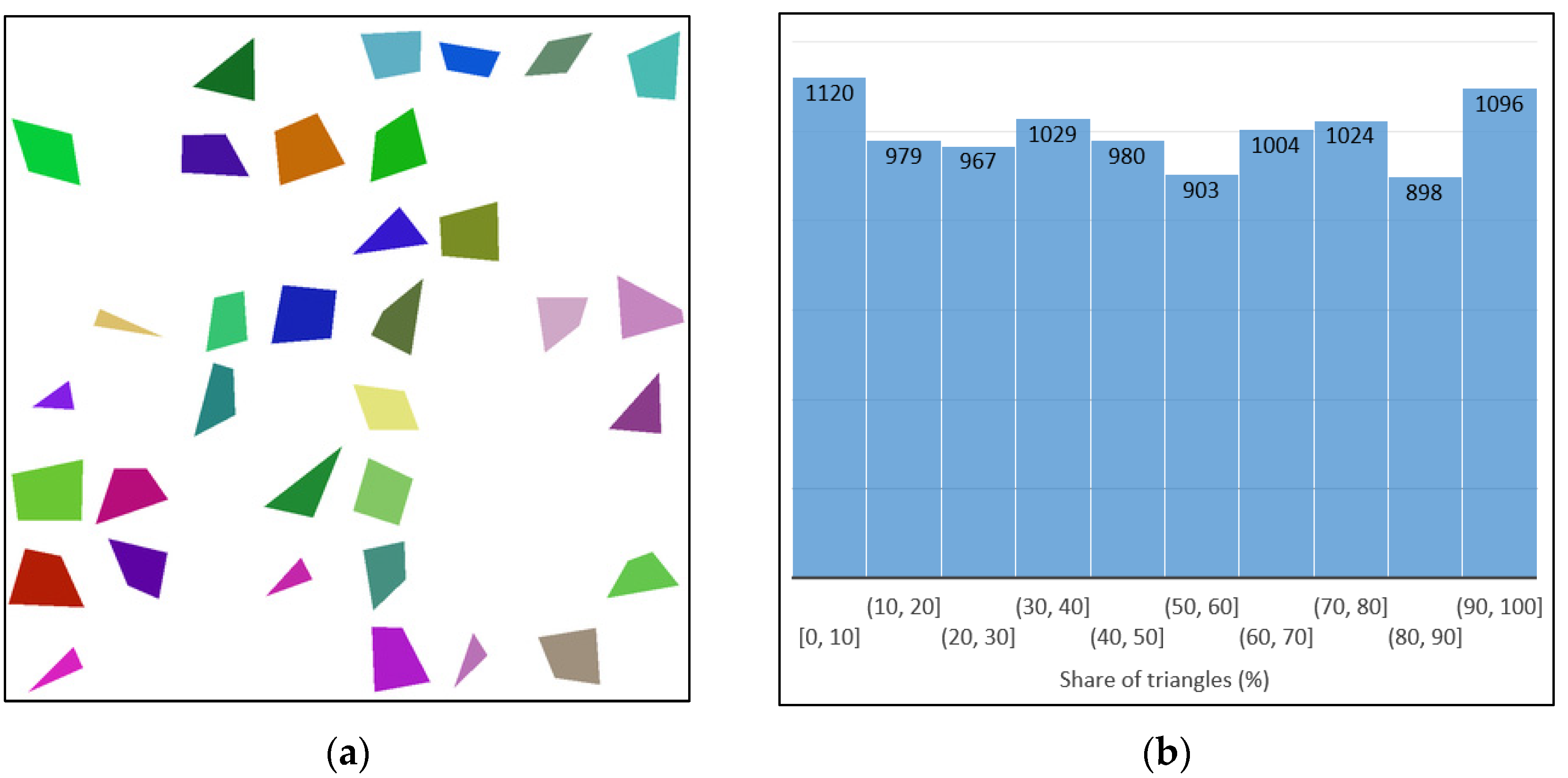
2.1.1. Toy Dataset (TOYds)

The artificially generated dataset consists of 10,000 RGB images. Each image is 1024 × 1024 pixels in size and contains a random number of triangles and quadrilaterals of different colors and sizes. All the quadrilaterals are convex, with interior angles that measure less than 150 degrees each. For each image, the share of triangles in the total number of objects was calculated, which will represent the ground truth during the experiment.

Figure 1 shows a sample image, as well as the distribution of the share (percentage) of triangles in all images in the dataset. Images contain between 8 and 62 objects (triangles or quadrilaterals), including between 0 and 60 triangles, respectively. In other words, the share of triangles is between 0% and 100%.

To check the impact that the size of the dataset has on the performance of the selected models, an additional dataset with 25,000 examples was generated on the same principles (TOY*ds).

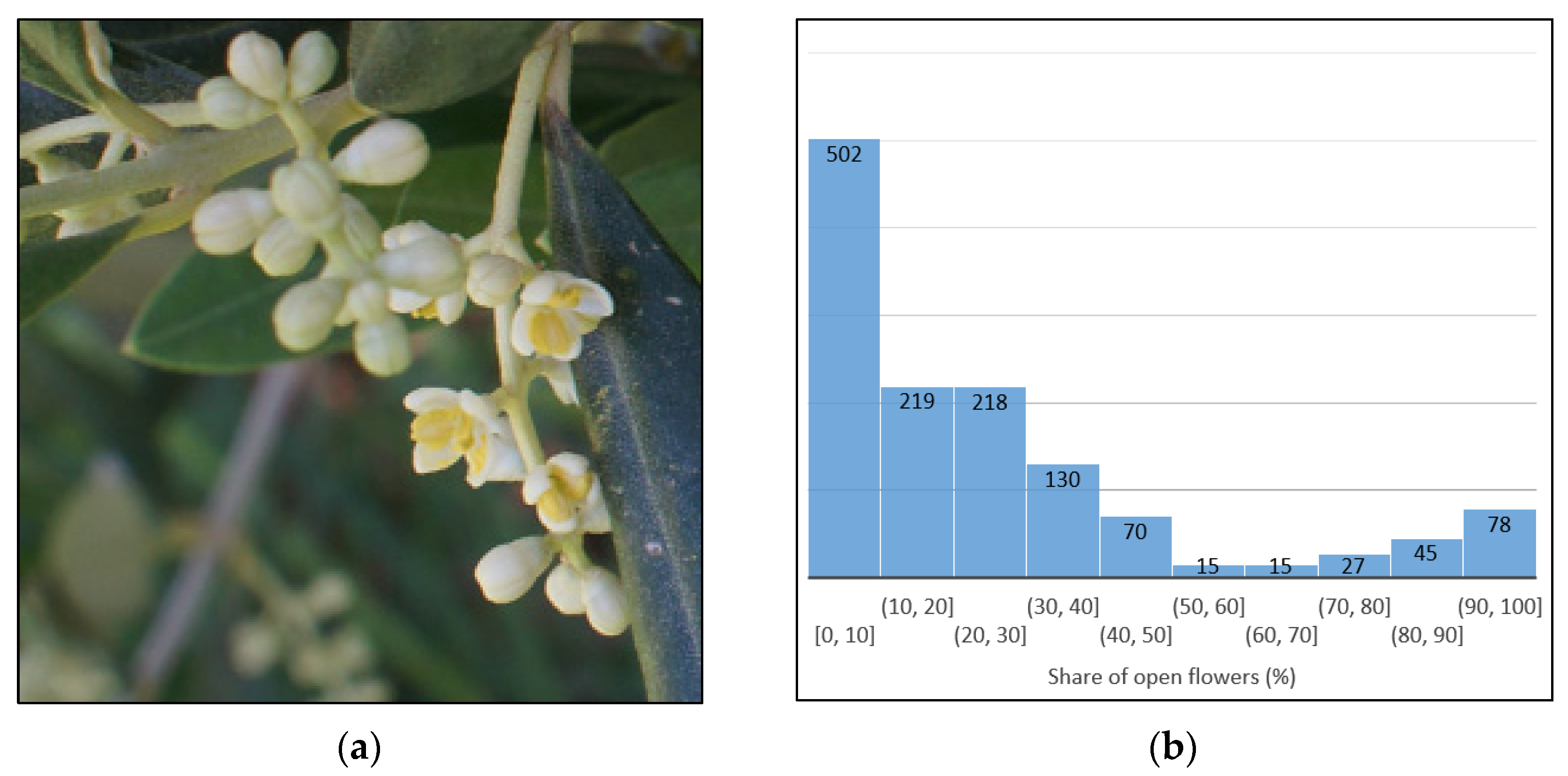
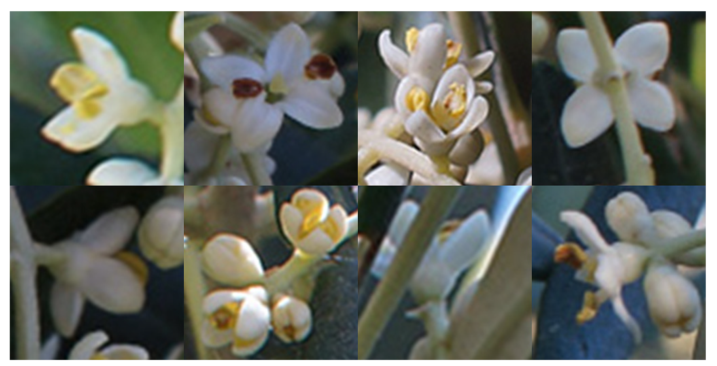
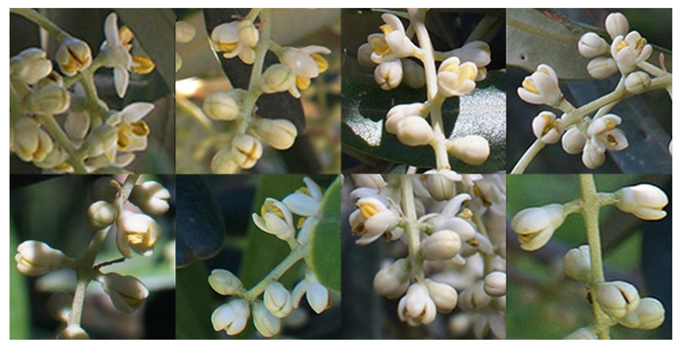
2.1.2. Olive Flowering Phenophases Dataset (OFPds)

Images in this dataset show olive canopies during different stages of flowering. We derived a total of 1314 images, 256 × 256 pixels in size, from a dataset we collected in an olive grove in southern Croatia [28].

Human expert annotators provided the ground truth data, made up of percentages of open flowers. They counted the total number of flowers in each image, as well as the number of open flowers per image. An example of an image from the dataset is shown in Figure 2, along with the distribution of the percentage of open flowers (between 0% and 100%).

It should be emphasized that open flowers may visually vary to a great degree, and that sometimes they are not easy to spot, depending on the angle and distance of the camera, the lighting, objects obstructing the view of the flowers, and other conditions. Figure 3 shows various examples of open flowers.

As had been expected, the number of samples in this dataset proved to be insufficient during the experiment, as the original dataset with 1000 images was insufficient to successfully carry out the learning phase. This is why we used data augmentation to generate new artificial learning examples: We applied various geometric image distortion techniques at random, such as translating, image rotation, zooming, and color modifications. This resulted in an increase in the size of the training dataset to 8509 images.

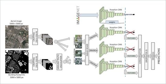
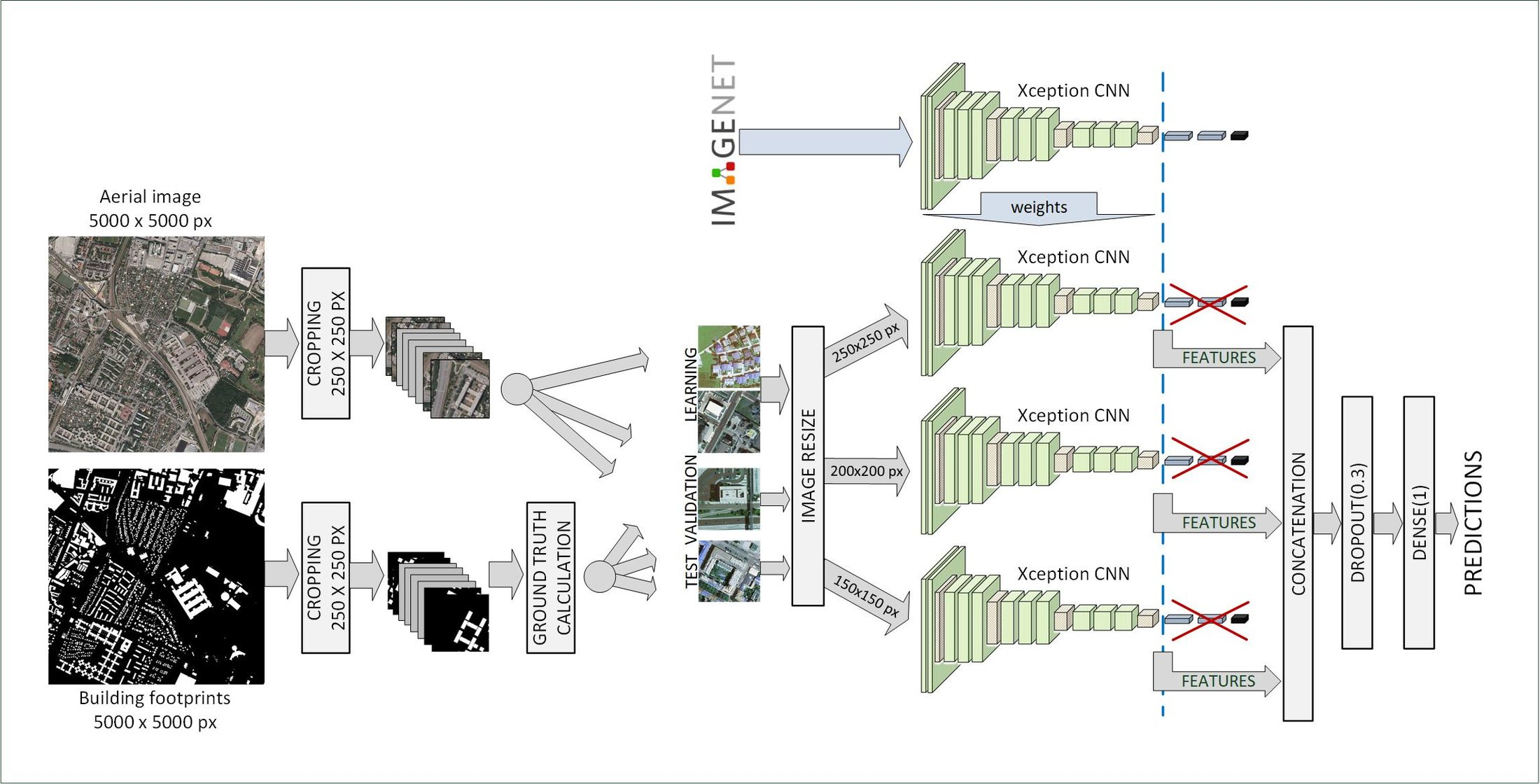
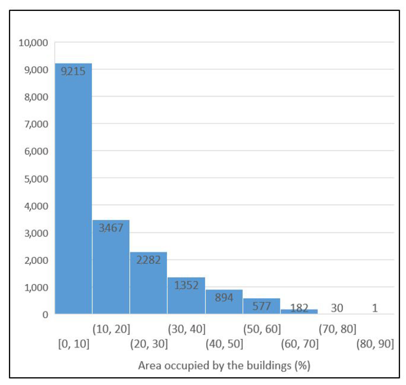
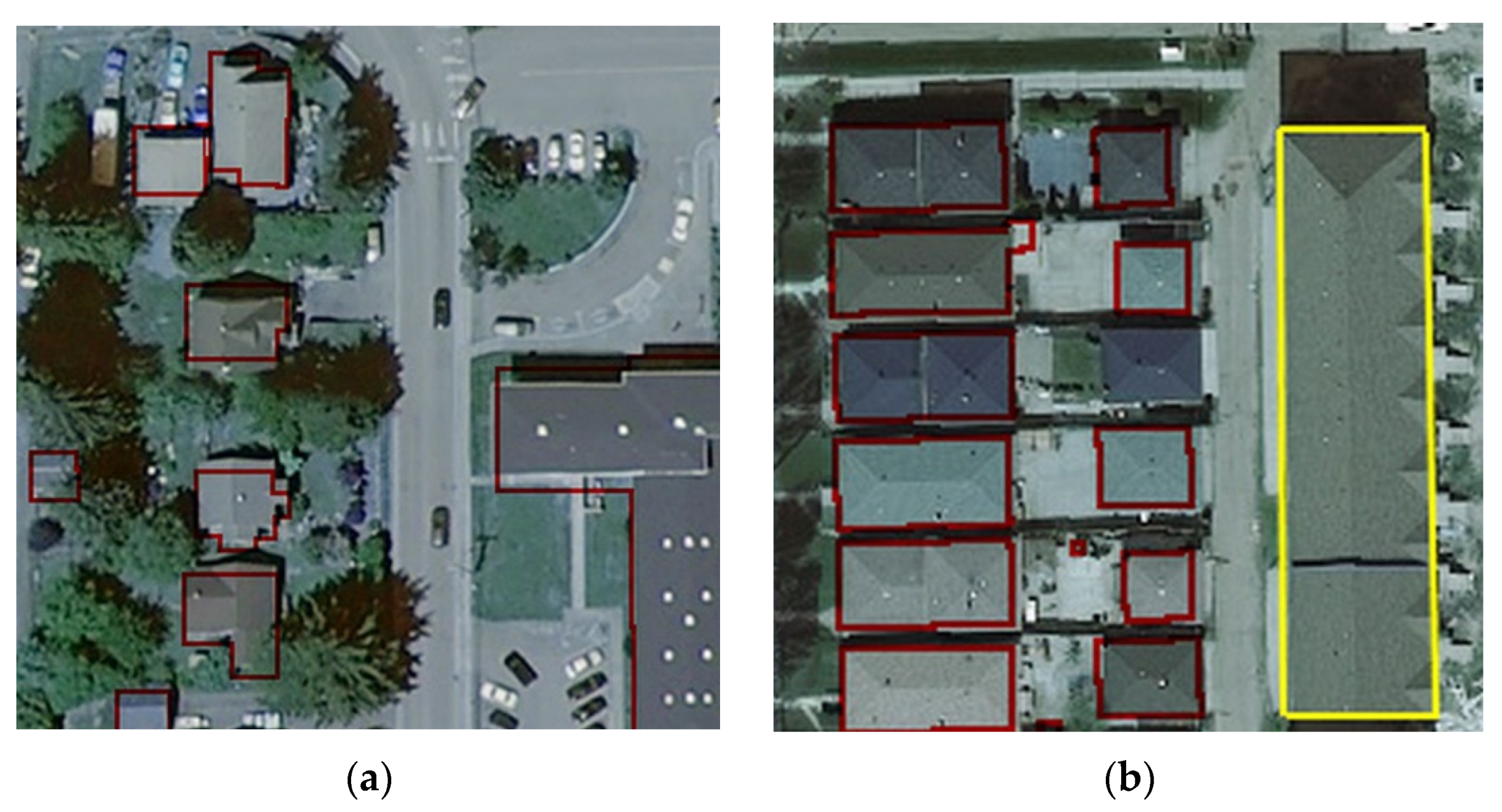
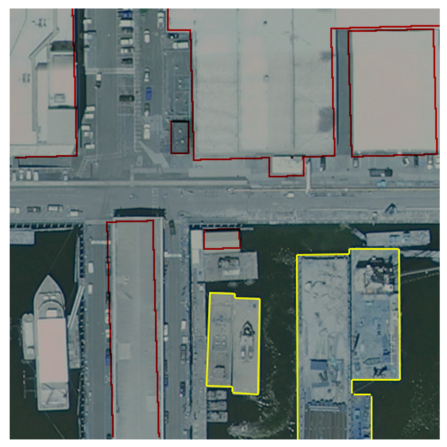
2.1.3. Aerial Image labeling Dataset (AILds)

This dataset is derived from the Inria aerial image labeling dataset, used in [29]. Original images are 5000 × 5000 pixels in size. The authors divided the semantic classes of this dataset into “building” and “not building”. To achieve their goal, the authors had to extract building footprints from the cadaster, which resulted in a semantic segmentation mask for each image.

During the preprocessing phase, the original image and its corresponding segmentation mask were divided into smaller subimages (250 × 250 pixels). In the next step, we used the black-and-white mask to calculate the percentage of the image area occupied by the buildings. In the end, a total of 18,000 images were available for the experiment.

An example of an image from the dataset is shown in Figure 4, as well as the corresponding segmentation mask. The distribution of the percentages of the image area occupied by the buildings is shown in Figure 5.

2.2. Methodology and Architectures

To prove the hypothesis that CNNs can successfully learn and interpret the concept of proportions for a very wide range of datasets, we tested a number of diverse architectures:

• Vanilla deep regression;
• General-purpose networks (e.g., VGG-19, Xception, InceptionResnetV2, etc.) modified for regression tasks;
• General-purpose networks in transfer learning mode, modified for regression tasks;
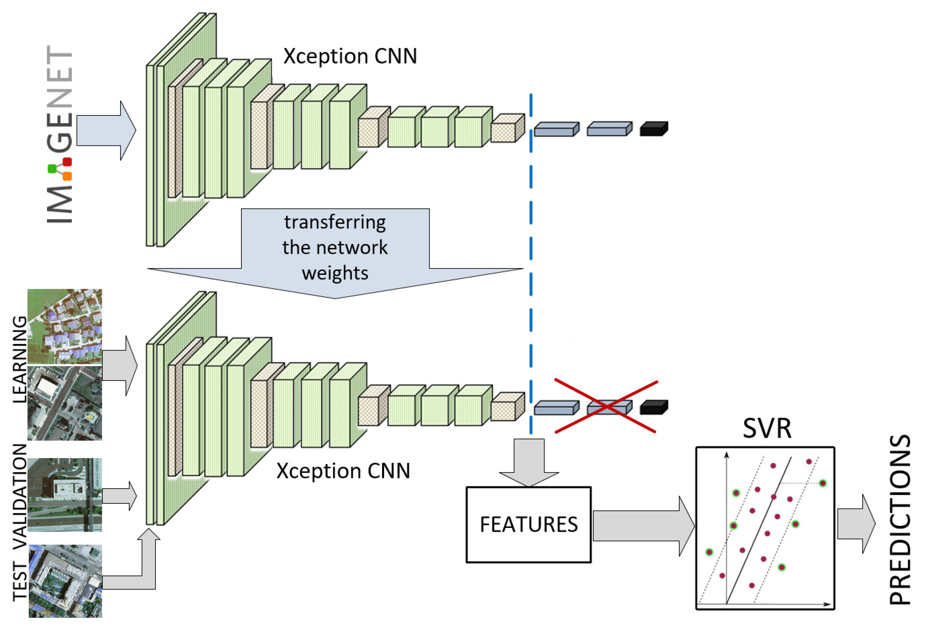
• Hybrid architectures (The CNN works as a trainable feature extractor, while the machine learning algorithm (e.g., SVR) performs as a regressor);
• Deep ensemble models for regression.

Although the majority of the models could be further adapted to the corresponding dataset with minor changes in the architecture, no additional adjustments were made for better comparison possibilities.

CNN training was implemented with the Keras [30] and TensorFlow [31] deep learning frameworks. We used a workstation equipped with an AMD Ryzen Threadripper 3960X CPU and NVIDIA GeForce RTX 3090 with 24 GB memory, with Linux Ubuntu 20.04 as the used OS.

An early stopping and a model checkpoint were used as a callback function. Early stopping interrupts the training process if there is no improvement of the validation loss after a defined number of epochs (with a default early stopping patience set to 15 epochs). The model checkpoint is used to save the best model if and once the validation loss decreases.

2.2.1. Vanilla Deep Regression

In this set of experiments, we compared the vanilla deep regression model (custom CNN with a regression top layer) with other models that are partly or entirely based on established algorithms. The architecture is based on VGG-16 and VGG-19 architectures [32], where the size of the applied network is the result of numerous experiments, including the grid-search used to find the optimal hyperparameters of a model. The values of the notable hyperparameters are as follows: The number of epochs is 100; mini-batch size is 32; learning rate is 0.001; Adam optimizer [33] and early stopping patience 15. For comparison purposes, we later used the same hyperparameter settings for all proposed models. It should be noted that other optimizers were also tested, where the best performance was achieved by Adam, alternating with RMSprop [34] in the first place for individual datasets and models.

The layers configuration of the vanilla deep regression model is as follows:

Conv2D(64) → ACT(ReLU) → BN → Conv2D(64) → ACT(ReLU) → BN → MP() → DR(0.1) → Conv2D(128) → ACT(ReLU) → BN → Conv2D(128) → ACT(ReLU) → BN → MP() → DR(0.2) → Conv2D(256) → ACT(ReLU) → BN → Conv2D(256) → ACT(ReLU) → BN → MP() → DR(0.2) → Conv2D(512) → ACT(ReLU) → BN → Conv2D(512) → ACT(ReLU) → BN → MP() → DR(0.2) → Conv2D(1024) → ACT(ReLU) → BN → Conv2D(1024) → ACT(ReLU) → BN → MP() → DR(0.3) → GAP() → DR(0.5) → DN(1) → ACT(ReLU_100)

where Conv2D(n) denotes the 2D convolution layer with n filters, ACT() denotes the activation function, BN denotes the batch normalization layer, MP denotes the max pooling layer, GAP denotes a 2D global average pooling layer, and FL denotes a flatten layer and DN(n) denotes a dense layer.

Since a proportion is the comparison of a part to the whole, it can have a value ranging from 0 to 1 (i.e., between 0% and 100%). Therefore, the original ReLU (rectified linear unit) activation function is modified (ReLU_100) as follows:

$$f\left(x\right)=\{\begin{array}{c}0, if x<0\hfill \\ x, if x\ge 0 \mathrm{and} x\le 100\hfill \\ 100, if x>100\hfill \end{array}$$

(1)

2.2.2. General-Purpose Networks

We tested several general purpose CNNs, where fully connected top layer structures were adjusted for regression. Finally, we chose three algorithms since they can be considered representatives of this group of algorithms: VGG-19 [32], Xception [35], and InceptionResnetV2 [36]. Several different top layer configurations were tested, where the choice was finally narrowed down to the following configurations:

(a)

GAP() → DR(0.3) → DN(1) → ACT(ReLU_100)

(b)

FL → DN(1024)→ BN → DR(0.5) → DN(128) → BN → DR(0.5) → DN(1) → ACT(ReLU_100)

By comparing the models’ performance on all three datasets, the first configuration was used in most cases.

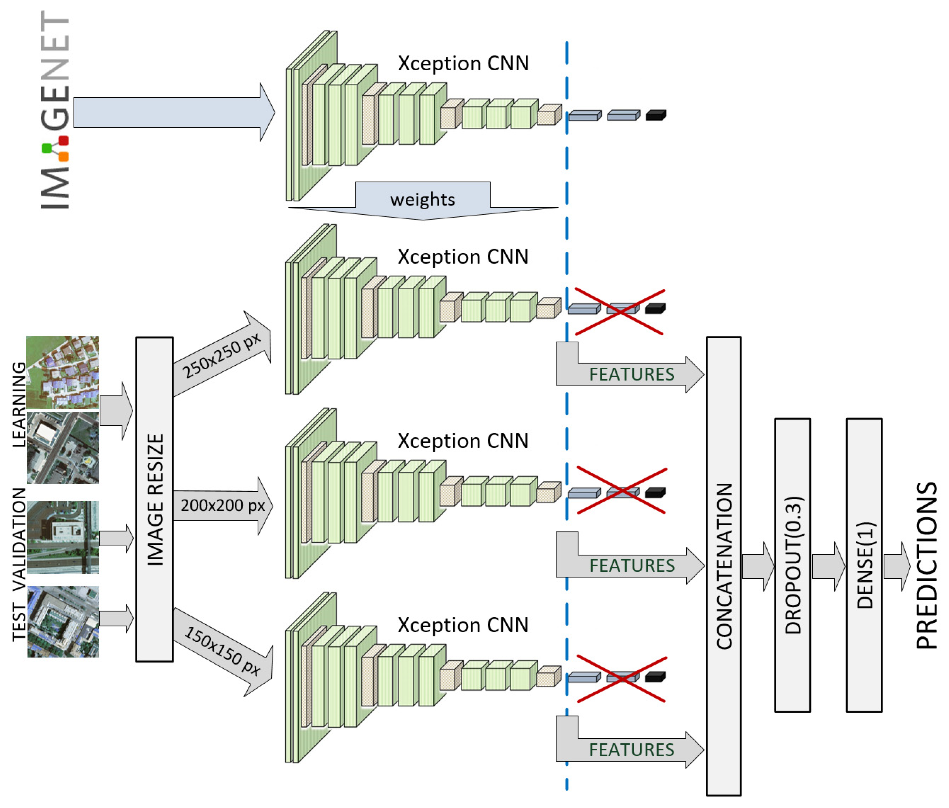
2.2.3. General-Purpose Networks in Transfer Learning Mode

We also compared learning from scratch to the application of transfer learning [37], as an indispensable tool in situations with insufficient training data. The goal is to try to transfer the knowledge from the source domain to the target domain, reusing the part of the network that was pre-trained in the source domain. e.g., as a weight initialization scheme. ImageNet [38] trained features are the most popular starting point for transfer task fine-tuning. In [39], the authors concluded that there is still no definitive answer to the question “What makes ImageNet good for transfer learning?”, but it is obvious that traditional CNN architectures can extract high-quality generic low/middle level features from an ImageNet dataset.

An additional useful feature is that we can freeze a certain part of the network. This is used primarily for preserving the low-level features that are built in the first layers of the network. During the training phase, the transferred weights can remain frozen at their initial values or trained together with the random weights (fine-tuning). As we used transfer learning from a completely different domain (ImageNet), we decided to fine-tune the layers instead of freezing them.

The previously mentioned models have an increased generalization ability across domains. Figure 6 shows that additional hyperparameter tuning can resolve overfitting and underfitting to a significant degree.

2.2.4. Hybrid Architectures

In the proposed approach, we used the CNN’s convolutional layers, with the pre-trained ImageNet weights, to extract features which are used to train the machine learning regression algorithm.

In our experiment, we used bottleneck features to train the representatives of regression models, namely support vector regression (SVR) [40] and random forest regressor (RFR) [41]. The concept of the experiment (Xception + SVR variant) is shown in Figure 7.

2.2.5. Deep Ensemble Models for Regression

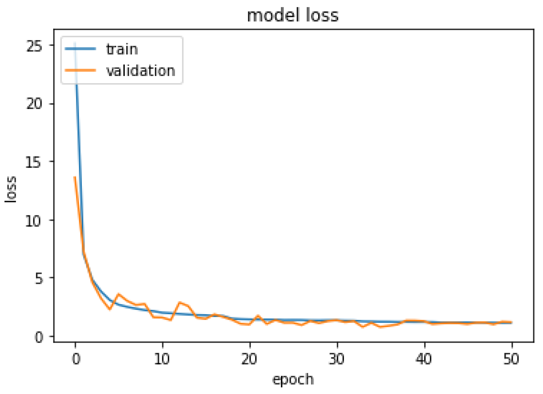
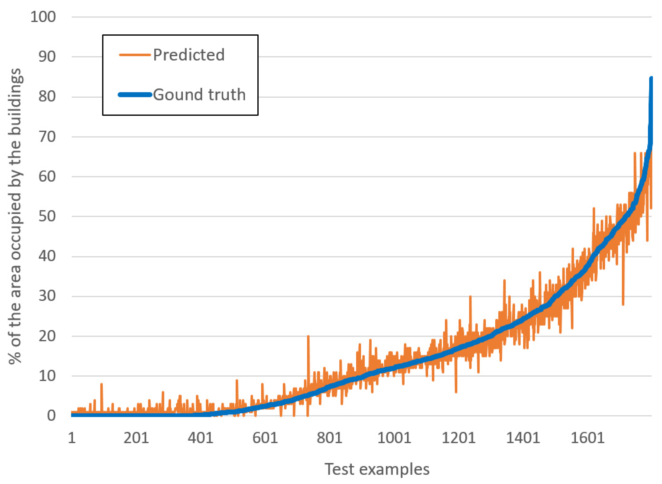
Ensemble methods can improve the predictive performance of a single model by training multiple models and combining their predictions [42]. Deep ensemble learning [43] combines deep learning models and ensemble learning so that the final model has a better generalization performance.

Still, extracting objects and details from images can be challenging due to their highly variable shape, size, color, and texture. To improve this, we proposed an ensemble model involving a multichannel CNN. Each channel is comprised of the input layer that defines the various sizes of input images, focusing on a particular scale. All channels share the standard CNN architecture in the transfer mode with the same set of filter parameters. The outputs from the three channels are concatenated and processed by dropout and dense layers (Figure 8). This architecture is expected to extract more robust features, i.e., to have greater resilience against large variations in object size.

3. Results

During the experiment, we tested hundreds of markedly different approaches and architectures, and the results we obtained with the selected typical use cases are presented further in this manuscript.

The performance of the predictions was evaluated using the coefficient of determination R², root mean square error (RMSE), and mean absolute error (MAE) metrics:

$$MAE=\frac{1}{N}{\displaystyle \sum }_{i=1}^N\left|y_i-{\widehat{y}}_i\right|$$

(2)

$$RMSE=\sqrt{\frac{1}{N}{\displaystyle \sum }_{i=1}^N{\left(y_i-{\widehat{y}}_i\right)}^2}$$

(3)

$$R^2=1-\frac{{{\displaystyle \sum }}_{i=1}^N{\left(y_i-{\widehat{y}}_i\right)}^2}{{{\displaystyle \sum }}_{i=1}^N{\left(y_i-{\overline{y}}_i\right)}^2}$$

(4)

where y_i is the ground-truth value, ŷ_i is the predicted data, ȳ is the mean of ground truth for all samples, and N is the number of testing samples.

We can draw the following conclusions based on the experiments conducted with CNNs listed in

Table 1. The prediction performance of the CNN-based models on the test datasets.

Dataset (Samples)	Model	MAE	RMSE	R2
TOYds (10,000)	vanilla CNN	1.26	1.84	0.983
	VGG-19 (scratch)	3.26	4.83	0.971
	VGG-19 (transfer)	2.68	3.62	0.985
	Xception (scratch)	0.69	0.93	0.883
	Xception (transfer)	0.37	0.56	0.998
	InceptionResNetV2 (scratch)	0.90	1.29	0.997
	InceptionResNetV2 (transfer)	0.42	0.60	0.998
TOY*ds (25,000)	vanilla CNN	0.23	0.29	0.998
	VGG-19 (scratch)	1.83	3.21	0.989
	VGG-19 (transfer)	1.25	2.88	0.991
	Xception (scratch)	0.45	1.69	0.998
	Xception (transfer)	0.21	0.27	0.999
	InceptionResNetV2 (scratch)	0.37	0.53	0.999
	InceptionResNetV2 (transfer)	0.17	0.25	0.998
OFPds (1314)	vanilla CNN	6.95	10.87	0.817
	VGG-19 (scratch)	8.72	12.56	0.724
	VGG-19 (transfer)	5.66	8.44	0.892
	Xception (scratch)	7.85	8.74	0.875
	Xception (transfer)	5.43	8.54	0.890
	InceptionResNetV2 (scratch)	8.78	13.12	0.711
	InceptionResNetV2 (transfer)	5.38	8.34	0.956
OFPds augmented (8509)	vanilla CNN	3.45	5.68	0.954
	VGG-19 (scratch)	3.90	6.95	0.927
	VGG-19 (transfer)	3.56	5.61	0.952
	Xception (scratch)	6.25	9.49	0.864
	Xception (transfer)	3.28	5.64	0.952
	InceptionResNetV2 (scratch)	4.03	6.62	0.933
	InceptionResNetV2 (transfer)	2.90	4.44	0.970
AILds (18,000)	vanilla CNN	2.13	3.98	0.939
	VGG-19 (scratch)	2.27	4.46	0.923
	VGG-19 (transfer)	1.77	3.39	0.956
	Xception (scratch)	2.96	5.74	0.873
	Xception (transfer)	1.69	3.13	0.962
	InceptionResNetV2 (scratch)	2.50	5.06	0.901
	InceptionResNetV2 (transfer)	1.75	3.37	0.956

: (1) for successful proportion estimation (MAE < 5), at least 10,000 examples are needed for a reasonable minimum dataset size; (2) a large training dataset can be created and prepared via data augmentation methods; (3) vanilla CNN optimized for regression, despite the relatively simple architecture and with fewer parameters than the VGG-19 model, can achieve acceptable results; (4) general-purpose networks (VGG-19, Xception, InceptionResnetV2, etc.), modified for regression tasks, perform approximately twice as well if pre-trained ImageNet weights are used.

We have shown that it is possible to improve the generalization of all proposed models with the controlled application of batch normalization [44] and dropout [45] techniques, but with caution and experimentation [46].

Table 2. The prediction performance of the hybrid/ensemble models on the test datasets.

Dataset (Samples)	Model	MAE	RMSE	R2
TOYds (10,000)	Xception + SVR	0.41	0.58	0.998
	Xception + RandomForestRegressor	0.45	0.69	0.998
	Xception * 3	0.49	0.69	0.998
	InceptionResNetV2 + SVR	0.56	0.75	0.997
	InceptionResNetV2 + RandomForestRegressor	0.44	0.65	0.998
	InceptionResNetV2 * 3	0.39	0.55	0.998
TOY*ds (25,000)	Xception + SVR	0.33	0.45	0.999
	Xception + RandomForestRegressor	0.24	0.43	0.999
	Xception * 3	0.21	0.33	0.999
	InceptionResNetV2 + SVR	0.32	0.47	0.999
	InceptionResNetV2 + RandomForestRegressor	0.27	0.46	0.999
	InceptionResNetV2 * 3	0.29	0.47	0.999
OFPds (1314)	Xception + SVR	5.99	8.88	0.881
	Xception + RandomForestRegressor	5.61	8.75	0.883
	Xception * 3	5.42	8.68	0.888
	InceptionResNetV2 + SVR	5.87	8.75	0.881
	InceptionResNetV2 + RandomForestRegressor	5.60	8.69	0.882
	InceptionResNetV2 * 3	5.35	8.41	0.902
OFPds augmented (8509)	Xception + SVR	3.52	5.21	0.959
	Xception + RandomForestRegressor	2.88	4.35	0.971
	Xception * 3	3.06	4.97	0.962
	InceptionResNetV2 + SVR	3.55	5.34	0.944
	InceptionResNetV2 + RandomForestRegressor	2.87	4.28	0.975
	InceptionResNetV2 * 3	2.75	3.87	0.979
AILds (18,000)	Xception + SVR	1.93	3.71	0.947
	Xception + RandomForestRegressor	1.78	3.30	0.958
	Xception * 3	1.62	3.12	0.982
	InceptionResNetV2 + SVR	1.96	3.85	0.940
	InceptionResNetV2 + RandomForestRegressor	1.79	3.45	0.954
	InceptionResNetV2 * 3	1.73	3.32	0.961

shows the results of hybrid and ensemble models based on Xception and InceptionResNetV2 architectures in transfer learning mode. Based on these results, we can further extend the abovementioned conclusions as follows: (5) using deep bottleneck features to train a machine learning algorithm (SVR, RFR) does not result in better performance than standard CNNs; (6) hybrid models involving a multichannel CNN (Xception * 3, InceptionResNetV2 * 3) show that ensemble regression methods are effective tools that improve the results and generalization performance of simple deep regression algorithms.

However, further assessment is needed for whether the improvement in performance, which rarely exceeds 10%, justifies the high number of parameters and computational cost. For example, the basic Xception algorithm (modified for regression, in transfer mode) has 66% fewer parameters than the multichannel Xception * 3 model, or 55% shorter duration of each epoch during the learning phase.

4. Summary and Discussion

The application of the proposed models on the olive flowering phenophases dataset shows that CNNs typically perform better than human experts, especially considering that, in the case of estimating thousands of images, this can be a mentally very demanding process.

The results should be also analyzed in the context of the reliability of determining the ground truth [47]. We used manual and automated methods to illustrate the importance of ground truth data design and use.

For the toy dataset, to guarantee the accuracy of the ground truth data, the exact share of triangles (ground truth) was computed during the image generation process. This fact, combined with 25,000 examples in the dataset, results in MAE values between 0.2 and 0.3 for the best models. However, we mentioned that the number of epochs (for all datasets) was limited during the experiment to a value of 100, in order to make the results comparable. With this in mind, after the experiment was finished, we tested some of the best-performing models further. We found that, if the maximum number of epochs is increased to 500 and early stopping patience to 30, an additional reduction of MAE to 0.14 can be achieved.

As already stated, for the olive flowering phenophases dataset, the ground truth is provided by human expert annotators. Generally speaking, flowers are defined as “open” when the reproductive parts are visible between or within unfolded or open flower parts. The application of this definition is not simple in practice, as can be seen in Figure 9.

To give an illustration of how this can be problematic in practice, we could say that there are a total of 20 buds and flowers in an image, but experts cannot agree on the classification of one particular flower. Thus, in this case, some of the experts would say that there are 10 open flowers, and others would say there are 11. Therefore, the percentages of open flowers are 50% and 55%, respectively. This means that the difference in estimate (ground truth) is 5%, just because of the differing classification of one flower. Even in this relatively simple example, the 5% difference is a noticeably larger percentage than the mistake percentages of the best-performing models.

Errors for the aerial image labeling dataset were also analyzed in detail (Figure 10).

As previously mentioned, a mask representing building footprints from the cadaster is available for the automated calculation of the percentage of the image area occupied by buildings. It is reasonable to assume that the ground truth thus defined should be reliable. However, the analysis of the results showed that this approach also has weaknesses. As can be seen in Figure 10, the examples of the overlapped images show that sporadically there are discrepancies between cadastral maps and aerial photographs. The first problem is that sometimes there is an offset of the building footprints (Figure 10a), which does not necessarily affect the result unless the building is only partially shown in the figure. A more significant problem arises in the case where there are buildings in the pictures that are not registered in the cadaster (Figure 10b). This results in instances with ground truth errors identified in training, validation and test datasets.

These are additional reasons why an MAE between 1 and 2 for the aerial image labeling dataset or MAE between 3 and 4 for the olive flowering phenophases dataset are considered to be excellent results.

Figure 11 shows the scatter plot of predicted values and the ground truth for the aerial images test dataset (1800 samples) and Xception * 3 model. Ground truth values (blue) are pre-sorted. Rare major discrepancies are mainly due to erroneous ground truth data.

Figure 12 shows an example of an error generated by the model itself. Building footprints from the cadaster (red) were indicated, but the model estimated that moored vessels (yellow) also represented buildings.

5. Conclusions

Precise proportion judgment is positively correlated with successful decision-making in a variety of decision tasks. It represents a particular type of ratio judgment in which a smaller magnitude is compared to a larger one. Therefore, the automation of this process could provide significant support in different processes, which is a topic that, to our knowledge, has not been systematically explored so far.

The experiments are designed to investigate in detail the possibilities of different deep regression architectures, by using three very different datasets that cover significantly different areas of application. Two datasets constitute our original contribution, while the third dataset is our adaptation of a publicly available dataset.

The performed experiments showed that the selected CNN models, adjusted for proportion judgment, predict proportions more reliably than human experts could, even without explicitly counting individual objects. Based on the results for the best models, and considering the coefficient of determination (>0.95) and the amount of errors (MAE < 2, RMSE < 3), we concluded that, with sufficient data and the use of transfer mode, we could achieve highly acceptable results. Still, the main problem remains the reliability of ground truth data.

The expanded toy dataset, with 25,000 examples and guaranteed reliability of the ground truth data, results in MAE values between 0.2 and 0.3 for the best models. With the maximum number of epochs increased to 500, an additional reduction of MAE to 0.14 can be achieved.

The two original datasets are a significant contribution of this project. We invested significant efforts in the development of these datasets. In the future, they could serve as reference data sources for the research and development of new methods for computer-assisted proportion judgment.

References

1. Chesney, D.; Bjalkebring, P.; Peters, E. How to estimate how well people estimate: Evaluating measures of individual differences in the approximate number system. Atten. Percept. Psycho. 2015, 77, 2781–2802. [Google Scholar] [CrossRef] [PubMed] [Green Version]
2. Hollands, J.G.; Dyre, B.P. Bias in proportion judgments: The cyclical power model. Psychol. Rev. 2000, 107, 500–524. [Google Scholar] [CrossRef] [PubMed]
3. Sheridan, T.B.; Ferrell, W.R. Man-Machine Systems: Information, Control, and Decision Models of Human Performance; The MIT Press: Cambridge, MA, USA, 1974. [Google Scholar]
4. Wickens, C.D.; Hollands, J.G.; Banbury, S.; Parasuraman, R. Engineering Psychology and Human Performance, 5th ed.; Routledge: Oxfordshire, UK, 2021. [Google Scholar] [CrossRef]
5. Lathuilière, S.; Mesejo, P.; Alameda-Pineda, X.; Horaud, R. A comprehensive analysis of deep regression. IEEE Trans. Pattern Anal. 2019, 42, 2065–2081. [Google Scholar] [CrossRef] [Green Version]
6. Khan, A.; Sohail, A.; Zahoora, U.; Qureshi, A.S. A survey of the recent architectures of deep convolutional neural networks. Artif. Intell. Rev. 2020, 53, 5455–5516. [Google Scholar] [CrossRef] [Green Version]
7. Shen, W.; Guo, Y.; Wang, Y.; Zhao, K.; Wang, B.; Yuille, A.L. Deep regression forests for age estimation. In Proceedings of the IEEE Conference on Computer Vision and Pattern Recognition, Salt Lake City, UT, USA, 18–23 June 2018; pp. 2304–2313. [Google Scholar]
8. Shi, L.; Copot, C.; Vanlanduit, S. A Deep Regression Model for Safety Control in Visual Servoing Applications. In Proceedings of the 2020 Fourth IEEE International Conference on Robotic Computing (IRC), Taichung, Taiwan, 9–11 November 2020; pp. 360–366. [Google Scholar]
9. Milicevic, M.; Zubrinic, K.; Grbavac, I.; Keselj, A. Ensemble Transfer Learning Framework for Vessel Size Estimation from 2D Images. In Proceedings of the International Work-Conference on Artificial Neural Networks, Gran Canaria, Spain, 12–14 June 2019; Springer: Cham, Switzerland, 2019; pp. 258–269. [Google Scholar]
10. Deng, J.; Bai, Y.; Li, C. A Deep Regression Model with Low-Dimensional Feature Extraction for Multi-Parameter Manufacturing Quality Prediction. Appl. Sci. 2020, 10, 2522. [Google Scholar] [CrossRef] [Green Version]
11. Gao, J.; Zhang, T.; Yang, X.; Xu, C. P2T: Part-to-target tracking via deep regression learning. IEEE Trans. Image Process 2018, 27, 3074–3086. [Google Scholar] [CrossRef]
12. Zhong, Z.; Li, J.; Zhang, Z.; Jiao, Z.; Gao, X. An attention-guided deep regression model for landmark detection in cephalograms. In Proceedings of the International Conference on Medical Image Computing and Computer-Assisted Intervention, Shenzhen, China, 13–17 October 2019; Springer: Cham, Switzerland, 2019; pp. 540–548. [Google Scholar]
13. Fang, C.; Huang, J.; Cuan, K.; Zhuang, X.; Zhang, T. Comparative study on poultry target tracking algorithms based on a deep regression network. Biosyst. Eng. 2020, 190, 176–183. [Google Scholar] [CrossRef]
14. Wang, Q.; Yang, D.; Li, Z.; Zhang, X.; Liu, C. Deep regression via multi-channel multi-modal learning for pneumonia screening. IEEE Access 2020, 8, 78530–78541. [Google Scholar] [CrossRef]
15. Wang, Q.; Wan, J.; Li, X. Robust hierarchical deep learning for vehicular management. IEEE Trans. Veh. Technol. 2018, 68, 4148–4156. [Google Scholar] [CrossRef]
16. Salehi, S.S.M.; Khan, S.; Erdogmus, D.; Gholipour, A. Real-time deep pose estimation with geodesic loss for image-to-template rigid registration. IEEE Trans. Med. Imaging 2018, 38, 470–481. [Google Scholar] [CrossRef]
17. Abdi, A.M. Land cover and land use classification performance of machine learning algorithms in a boreal landscape using Sentinel-2 data. Gisci. Remote Sens. 2020, 57, 1–20. [Google Scholar] [CrossRef] [Green Version]
18. Jia, K.; Liang, S.; Gu, X.; Baret, F.; Wei, X.; Wang, X.; Yao, Y.; Yang, L.; Li, Y. Fractional vegetation cover estimation algorithm for Chinese GF-1 wide field view data. Remote Sens. Environ. 2016, 177, 184–191. [Google Scholar] [CrossRef]
19. Yu, R.; Li, S.; Zhang, B.; Zhang, H. A Deep Transfer Learning Method for Estimating Fractional Vegetation Cover of Senti-nel-2 Multispectral Images. IEEE Geosci. Remote Sens. 2021, 19, 1–5. [Google Scholar] [CrossRef]
20. Carpenter, G.A.; Gopal, S.; Macomber, S.; Martens, S.; Woodcock, C.E. A neural network method for mixture estimation for vegetation mapping. Remote Sens. Environ. 1999, 70, 138–152. [Google Scholar] [CrossRef] [Green Version]
21. Mohammed-Aslam, M.A.; Rokhmatloh-Salem, Z.E.; Javzandulam, T.S. Linear mixture model applied to the land-cover classification in an alluvial plain using Landsat TM data. J. Environ. Inform. 2006, 7, 95–101. [Google Scholar] [CrossRef] [Green Version]
22. Blinn, C.E. Increasing the Precision of Forest Area Estimates through Improved Sampling for Nearest Neighbor Satellite Image Classification. Ph.D. Thesis, Virginia Tech, Blacksburg, VA, USA, 2005. [Google Scholar]
23. Wu, B.; Li, Q. Crop planting and type proportion method for crop acreage estimation of complex agricultural landscapes. Int. J. Appl. Earth Obs. 2012, 16, 101–112. [Google Scholar] [CrossRef]
24. Drake, N.A.; Mackin, S.; Settle, J.J. Mapping vegetation, soils, and geology in semiarid shrublands using spectral matching and mixture modeling of SWIR AVIRIS imagery. Remote Sens. Environ. 1999, 68, 12–25. [Google Scholar] [CrossRef]
25. Gilbert, M.; Grégoire, J.C. Visual, semi-quantitative assessments allow accurate estimates of leafminer population densities: An example comparing image processing and visual evaluation of damage by the horse chestnut leafminer Cameraria ohridella (Lep., Gracillariidae). Jpn. J. Appl. Entomol. Z 2003, 127, 354–359. [Google Scholar] [CrossRef]
26. Alaiz-Rodrıguez, R.; Alegre, E.; González-Castro, V.; Sánchez, L. Quantifying the proportion of damaged sperm cells based on image analysis and neural networks. Proc. SMO 2008, 8, 383–388. [Google Scholar]
27. Zhu, Q.; Chen, J.; Wang, L.; Guan, Q. Proportion Estimation for Urban Mixed Scenes Based on Nonnegative Matrix Factorization for High-Spatial Resolution Remote Sensing Images. IEEE J. Sel. Top. Appl. Earth Obs. Remote Sens. 2021, 14, 11257–11270. [Google Scholar] [CrossRef]
28. Milicevic, M.; Zubrinic, K.; Grbavac, I.; Obradovic, I. Application of deep learning architectures for accurate detection of olive tree flowering phenophase. Remote Sens. 2020, 12, 2120. [Google Scholar] [CrossRef]
29. Maggiori, E.; Tarabalka, Y.; Charpiat, G.; Alliez, P. Can semantic labeling methods generalize to any city? The inria aerial image labeling benchmark. In Proceedings of the IEEE International Geoscience and Remote Sensing Symposium (IGARSS), Fort Worth, TX, USA, 23–28 July 2017; pp. 3226–3229. [Google Scholar]
30. Chollet, F. Deep Learning with Python; Simon and Schuster: New York, NY, USA, 2021. [Google Scholar]
31. Abadi, M.; Agarwal, A.; Barham, P.; Brevdo, E.; Chen, Z.; Citro, C.; Corrado, G.S.; Davis, A.; Dean, J.; Devin, M.; et al. Tensorflow: Large-scale machine learning on heterogeneous distributed systems. arXiv 2016, arXiv:1603.04467. [Google Scholar]
32. Simonyan, K.; Zisserman, A. Very deep convolutional networks for large-scale image recognition. arXiv 2014, arXiv:1409.1556. [Google Scholar]
33. Kingma, D.P.; Ba, J. Adam: A method for stochastic optimization. arXiv 2014, arXiv:1412.6980. [Google Scholar]
34. Tieleman, T.; Hinton, G. Lecture 6.5-rmsprop: Divide the gradient by a running average of its recent magnitude. COURSERA Neural Netw. Mach. Learn. 2012, 4, 26–31. [Google Scholar]
35. Chollet, F. Xception: Deep learning with depthwise separable convolutions. In Proceedings of the IEEE Conference on Computer Vision and Pattern Recognition, Honolulu, HI, USA, 21–26 July 2017; pp. 1251–1258. [Google Scholar]
36. Szegedy, C.; Ioffe, S.; Vanhoucke, V.; Alemi, A.A. Inception-v4, inception-resnet and the impact of residual connections on learning. In Proceedings of the Thirty-First AAAI Conference on Artificial Intelligence, San Francisco, CA, USA, 4–9 February 2017. [Google Scholar]
37. Tan, C.; Sun, F.; Kong, T.; Zhang, W.; Yang, C.; Liu, C. A survey on deep transfer learning. In Proceedings of the International Conference on Artificial Neural Networks, Rhodes, Greece, 4–7 October 2018; Springer: Cham, Switzerland, 2018; pp. 270–279. [Google Scholar]
38. Krizhevsky, A.; Sutskever, I.; Hinton, G.E. Imagenet classification with deep convolutional neural networks. Adv. Neural Inf. Process. Syst. 2012, 25, 1097–1105. [Google Scholar] [CrossRef]
39. Huh, M.; Agrawal, P.; Efros, A.A. What makes ImageNet good for transfer learning? arXiv 2016, arXiv:1608.08614. [Google Scholar]
40. Schölkopf, B.; Smola, A.J.; Williamson, R.C.; Bartlett, P.L. New support vector algorithms. Neural Comput. 2000, 12, 1207–1245. [Google Scholar] [CrossRef]
41. Breiman, L. Random forests. Mach. Learn. 2001, 45, 5–32. [Google Scholar] [CrossRef] [Green Version]
42. Sagi, O.; Rokach, L. Ensemble learning: A survey. Wires Data Min. Knowl. 2018, 8, e1249. [Google Scholar] [CrossRef]
43. Ganaie, M.A.; Hu, M. Ensemble deep learning: A review. arXiv 2021, arXiv:2104.02395. [Google Scholar]
44. Ioffe, S.; Szegedy, C. Batch normalization: Accelerating deep network training by reducing internal covariate shift. In Proceedings of the International Conference on Machine Learning, Lille, France, 6–11 July 2015; PMLR: London, UK, 2015; pp. 448–456. [Google Scholar]
45. Srivastava, N.; Hinton, G.; Krizhevsky, A.; Sutskever, I.; Salakhutdinov, R. Dropout: A simple way to prevent neural networks from overfitting. J. Mach. Learn. Res. 2014, 15, 1929–1958. [Google Scholar]
46. Garbin, C.; Zhu, X.; Marques, O. Dropout vs. batch normalization: An empirical study of their impact to deep learning. Multimed. Tools Appl. 2020, 79, 12777–12815. [Google Scholar] [CrossRef]
47. Krig, S. Ground truth data, content, metrics, and analysis. In Computer Vision Metrics; Springer: Berlin/Heidelberg, Germany, 2016; pp. 247–271. [Google Scholar] [CrossRef]
Figure 1. Toy dataset (a) Sample image; (b) Distribution of the share (percentage) of triangles for all images in the dataset.
Futureinternet 14 00100 g001
Figure 2. Olive flowering phenophases dataset (a) Sample image; (b) Distribution of the share (percentage) of open flowers for all images in the dataset.
Futureinternet 14 00100 g002
Figure 3. Illustration of the variations of open flowers.
Futureinternet 14 00100 g003
Figure 4. Aerial image labeling dataset (a) Sample image; (b) Semantic segmentation mask, buildings are marked in white.
Futureinternet 14 00100 g004
Figure 5. The percentage of the image area occupied by buildings.
Futureinternet 14 00100 g005
Figure 6. Training loss and validation loss curves of InceptionResnetV2 in transfer learning mode.
Futureinternet 14 00100 g006
Figure 7. Hybrid architecture—Xception (feature extraction) + SVR (regression).
Futureinternet 14 00100 g007
Figure 8. Deep ensemble model for regression—3 × Xception.
Futureinternet 14 00100 g008
Figure 9. Samples of transitions from buds to open flowers.
Futureinternet 14 00100 g009
Figure 10. Aerial images with marked building footprints from cadaster (red) (a) Building footprints have significant offset; (b) New building missing the footprint (yellow).
Futureinternet 14 00100 g010
Figure 11. Scatter plot of predicted values versus ground truth, for the aerial image labeling dataset, Xception * 3 model.
Futureinternet 14 00100 g011
Figure 12. Aerial image with marked building footprints from cadaster (red) and moored vessels (yellow).
Futureinternet 14 00100 g012