Flow Scheduling in Data Center Networks with Time and Energy Constraints: A Software-Defined Network Approach

Abstract

Flow scheduling in Data Center Networks (DCN) is a hot topic as cloud computing and virtualization are becoming the dominant paradigm in the increasing demand of digital services. Within the cost of the DCN, the energy demands associated with the network infrastructure represent an important portion. When flows have temporal restrictions, the scheduling with path selection to reduce the number of active switching devices is a NP-hard problem as proven in the literature. In this paper, an heuristic approach to schedule real-time flows in data-centers is proposed, optimizing the temporal requirements while reducing the energy consumption in the network infrastructure via a proper selection of the paths. The experiments show good performance of the solutions found in relation to exact solution approximations based on an integer linear programming model. The possibility of programming the network switches allows the dynamic schedule of paths of flows under the software-defined network management.

1. Introduction

Actual trends in computer applications development are oriented to the use of servers, data centers and virtualization to cope with the huge demand of digital services. In this context, networks become increasingly more complex and require better quality of service (QoS) in terms of the bandwidth, response time, throughput and latency, among others. Network administrators have been working in the concept of software defined networks (SDNs) to improve the QoS by separating the control plane from the data plane [1].

In this kind of network, the control of the network runs on a centralized server and not on individual networking devices, such as switches or routers. With this approach, network administrators are able to manage traffic flows implementing different policies oriented to provide load-balancing among servers, fault-recovery mechanisms when a path is broken, minimize the response time to users and reduce the energy demand of the data centers, among other optimal criteria. While in traditional networking devices, the administrator has to set up every device in the system, with SDN, the programming is done from a centralized controller for all the devices, and it may be changed dynamically based on the actual demands of the network.

The SDN paradigm is mainly powered by the Open Networking Foundation [2] with several first level companies as partners, such as Google and AT&T and more than one hundred members, including Cisco, arm, AMD, Nvidia and Microsoft. The proposed model for network management includes two interfaces.

The southbound is between the controller and the network infrastructure elements, and the northbound is between the controller and the network applications. Among the southbound protocols, OpenFlow [3] is the most developed and defines the way the switching and routing tables are configured. There are other approaches, such as network function virtualization and Network Virtualization [4,5,6] applied to DCN.

The considerable growth of cloud based applications has pushed the deployment of big data centers (DCN) around the world. These demand significant and increasing amounts of energy and these can be as great as the cost of the hardware involved [7]. Thus, energy saving in data centers is important not only for economical and environmental reasons but also for the sustainable growth of cloud computing [8]. The servers involved in DCN work with dynamic voltage scaling (DVS) [9] to reduce the energy consumption when there is low computing demand; however, the network infrastructure works continuously, and this represents about 20% of the energy consumed by the data center [10]. It is expected that DCNs will represent 20% of the world energy demand by 2025 [11]. This is a huge amount of electricity that a proper schedule and network administration can help to reduce.

The need to provide large connectivity among servers in a DCN impulses the weight of the network infrastructure in the final cost of the system. While servers can operate with energy-aware policies, such as reducing the voltage and clock operation frequency with DVS, switches and routers should be ready to work at all times, and thus the relative energy demands of the network infrastructure elements may be even higher than 20%. A first approach to reduce the energy demand of the network switches/routers will be to multiplex flows using only a reduced set of the possible paths and turning off or sleeping the elements not used.

Even if the approach may produce some good results, it is not necessarily true that such an approach will be the best. In fact, the switches may be operating for longer periods, while using other paths (switches) may reduce the transmission time and with this the energy demand. In DCN, several tasks are run in parallel in the servers, which requires exchanges of information. These exchanges are characterized as flows. As tasks in servers may have real-time constraints [12], the associated flows also have deadlines. Flow scheduling is a complex problem that has been proven to be NP-Hard [8]. It consists of deciding which flows should be transmitted through which paths in each instant to guarantee that none of the flows miss their deadlines and that the energy demand is kept to a minimum.

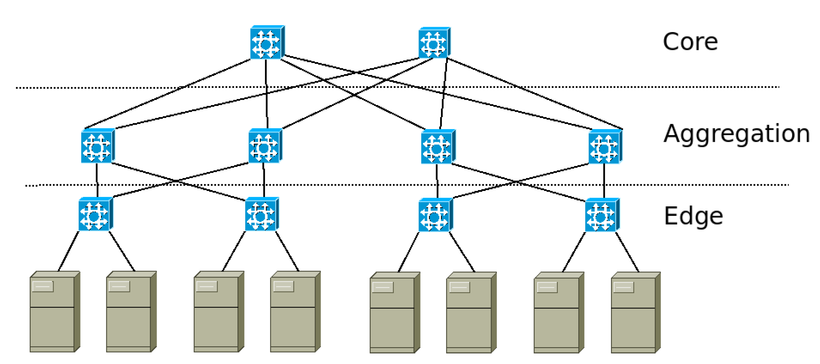
There are different kinds of topologies for DCN [4]. In this paper, the fat-tree [13] is used as it is the most accepted since it provides full connectivity among any pair of servers. It is based on three switching levels where each switch provides the same amount of input ports as output ports guaranteeing that any flow arriving into the switch will have an output link available. In Figure 1, a simple network with eight servers is shown.

Contribution: In this paper, we introduce an Integer Linear Programming (ILP) model to optimize the scheduling of real-time flows with energy aware considerations. The model can be solved with well-known tools, such as CPLEX. However, as it is an NP-hard problem, its exact solution is not possible when several servers are included in the DCN.

In order to obtain a valid schedule, the problem is solved using a heuristic approach in three steps designed and implemented by the authors. In the first step, the time scheduling is solved; in the second step, path allocation is performed; and finally, in the third stage, flows that were not scheduled in the first two steps are allocated. Experimental results show that the DCN can be scheduled in a short amount of time allowing for a dynamic operation of the system.

Organization: The rest of the paper is organized in the following way. In Section 2, previous works are discussed. After that, Section 3 introduces the real-time problem, and general scheduling considerations are provided. Section 4 presents the ILP model, and it is explained. The following Section 5, describes the proposed heuristics and the algorithms used. In Section 6, the different approaches are evaluated, and the results are compared. A brief discussion of the results is made in Section 7, and finally, in Section 8, conclusions are drawn, and future work lines are described.

2. Related Work

In [14], the authors present a survey on the load balancing problem in data centers and cloud servers under the SDN paradigm. This paper is useful as it shows that several issues still need to be studied. One of the aspects mentioned is the need to include the QoS provided to the flows while distributing the load. QoS can be measured by different aspects, such as the throughput, latency, allocated bandwidth and response time. In [15], the authors introduce an efficient dynamic load balancing scheme based on Nash bargaining for a distributed software-defined network. In [16], the v-Mapper framework is presented as a resource consolidation scheme that implements network resource-management concepts through software-defined networking (SDN) control features. The paper implements a virtual machine placement algorithm to reduce the communication costs while guaranteeing enough resources for the applications involved and a scheduling policy that aims to eliminate network load constraints. However, none of this proposals deal with energy and time constraints simultaneously.

The SDN concept is gaining space in different networking applications as it allows a rapid reconfiguration of the infrastructure to cope with changing scenarios. In [17], the Internet of Vehicles (IoV), is handled with this approach. The authors propose an autonomic software-defined vehicular architecture grounded on the synergy of Multi-access Edge Computing (MEC) and Network Functions Virtualization (NFV) along with a heuristic approach and an exact model based on linear programming to efficiently optimize the dynamic resource allocation of SDN controllers, thus, ensuring load balancing between controllers and employing reserve resources for tolerance in the case of demand variation.

Energy demands associated with cloud computing and data centers have three main components: servers, a cooling system and network devices. There are several papers regarding reducing the energy consumption of servers by implementing dynamic voltage and frequency scaling (DVFS) [9,18,19,20]. Usually, servers use multi-core processors, and these can be scheduled with different approaches to comply with time constraints and reduce energy consumption [21,22,23]. In this paper, we propose a heuristic to reduce the energy consumption of the network while keeping the flow QoS.

In [24], the authors propose flow scheduling in data centers operated with SDN infrastructure based on the energy consumption considering deadlines for the flow. Although this paper is close to our proposal, it differs in the type of optimization mechanism and in the way it is evaluated.

In [25], the authors present a load-balancing mechanism based on the response time of the server. The authors argue that the response time of the server is the main factor determining the user experience in the system. This is different from the approach proposed in this paper, as we also consider the energy consumption of the network during the scheduling of the flows.

In [8], the authors introduce a heuristic to optimize energy demand subject to complying flow deadlines. In our approach, the system is modelled with an ILP approach that facilitates the introduction of several objective functions.

In [26], the authors proposed an optimisation procedure for SDN based networks. However, the analysis is not centered in DCNs with fat-tree topologies but in open networks for standard data transport. The proposal includes the routing of information minimizing the use of switches allowing in this way the turning off or sleeping of infrastructure equipment.

Network architecture is an important aspect when considering flow scheduling with QoS and energy demand restrictions. One of the most used architectures is the fat-tree. It is organized in three switch layers: the edge, aggregation and core. Below the edge switches, the servers are connected [13,27]. Paths connecting servers can be chosen with different criteria, such as maximizing throughput, avoiding the use of shared links and reducing the number of active switches.

For this, Ref. [28] introduce a scalable and dynamic flow scheduling algorithm, and in [29], the authors propose the use of a limited number of core switches to accommodate the network traffic rates to save energy. In [30], the authors propose to sleep switches and routers for saving energy in the networks. Other works included in this approach are traffic equalization to distribute the flows or reduce the load of control protocols, such as OSPF [31,32].

In [33], the authors propose a distributed framework for SDNs called “Sieve”. The framework considers flow classes and network situation, i.e., links bandwidths and flows weights by periodically polling some of the network switches and sampling some of the network flows. The authors compare the real-time performance of their scheduling algorithm against the ones obtained with Hedera [28] and ECMP (Equal Cost MultiPath) [34] for different scenarios. The proposed scheduling algorithm is not optimal, does not include energy considerations and focuses entirely on the real time throughput of the DCNs flows. Finally, the authors do not show how their algorithm may scale with DCN size.

3. Real-Time Problem Description

In [12], a real-time system is defined as one in which at least one task should produce correct results before a certain instant named deadline. In [35], several scheduling policies were analysed based on task parameters, such as the priority, period, computation time and deadlines, and sufficient conditions were stated for the different policies. The analysis was done first for the case of multiple tasks running on a monoprocessor system. In [36], it was proven that the scheduling of messages in local area networks with a unique link was an isomorphous problem. Based on these previous results, in this paper, the notation is extended to analyse the flow scheduling in data centre networks.

A flow is a stream of data that is produced by a server and consumed by another one. There are different kinds of flows, such as multimedia ones, data files, cryptographic procedures and web search contents. Each flow $f=(o_f,d_f,t_f,p_f)$ has a source server $o_f$, a destination server $d_f$, a size or duration $t_f$ and a period $p_f$. As flows are assumed to be periodic, they can be seen as a stream of activations. For each activation k of flow f, $r_f^k$ is the instant at which it is released or becomes ready for being transmitted, $r_f^1=1$ and $r_f^k=r_f^{k-1}+p_f$ for $k>1$.

In addition, each activation has a deadline $v_f$ before which it must be sent. In a similar way, deadlines are also dynamic and are computed as $v_f^k=r_f^k+p_f$ The deadline is a requirement, it is determined by the kind of application associated with the flow, and its formal definition is beyond this work as this is a property of the flow as is the size.

A path in a DCN is a set of links and switches that communicate two different servers. In the fat-tree topology, all links are full duplex, and each server has several available paths to the rest of the servers in the DCN. However, there is only one link between it and the first level of switches named edge, as can be seen in Figure 1 [13]. This means that there is a restriction both in flows going out of the server as those arriving to it. Only one flow at a time can be transmitted or received on each server. The real-time analysis is limited to the last link because all other switches have the same amount of inputs as outputs guaranteeing that all the incoming flows have an output port.

The restriction in the last link limits the server capacity both for transmission and reception. The utilization factor or bandwidth requirement for each flow f can be computed as $u_f=\frac{t_f}{p_f}$. This relation provides the link occupancy or the percentage of time it is used by each flow. Clearly, the link capacity is limited to 1, and if it is overflowed, some flows will not comply with time restrictions. The last link can be analysed as a classical multitask/monoprocessor system as different flows have to be scheduled on a single link satisfying all deadlines. In [35], they proved the necessary conditions for the feasibility of this kind of systems, and it can be extended to this case as stated in Equation  (1), where $F_i^o$ and $F_i^d$ are the sets of flows with origin or destination on server i, respectively.

$${\displaystyle \sum _{\forall f\in F_i^o}}{u}_f\le 1\&\&{\displaystyle \sum _{\forall f\in F_i^d}}{u}_f\le 1\forall \mathrm{server} i$$

(1)

However, Equation (1) is not sufficient to guarantee the schedulability of the flows. In fact, servers eventually exchange data with many others. Thus, two servers sending flows to the same destination interfere between them, and it is not sufficient to consider the utilization factor demand on the individual servers. It is for this that the time and path scheduling should be global, because it is impossible to transmit a flow from a server if it cannot be received at the destination. This fact may introduce priority inversions at sending nodes where a flow with a relative deadline further away is scheduled before a more urgent one but is being blocked at the destination server.

The scheduling algorithm is abstracted from the application layer, which means that, at the network level, each flow can be identified by its origin, destination, size and period, regardless of the source or data format as stated at the beginning of this section. When one or more applications request different flows with the same source and destination servers, all flows are treated as independent ones. At each slot, however, the scheduler should choose one flow to send, and this decision is independent of the size of the flow but on the priority determined by the period or deadline.

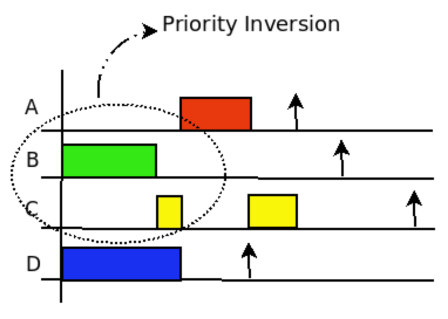
In the following example, there are three nodes interacting. Nodes 1 and 3 send flows to node 2. However, the priority of the flow with origin in 3 is higher than that of the flow with origin in 1. Server 1 also has other flows to different destinations.

Table 1. Flows description.

Flow	Source	Destination	Size	Period	Deadline
A	1	2	3	10	10
B	1	*	4	12	10
C	1	*	3	15	15
D	3	2	5	8	8

shows the flow identification, source, destination, size, period and deadline. In both nodes, the utilization factor is below 1. The symbol * indicates the destination is to some other server (different from 2) in the DCN.

As can be seen in the scheduling graph in Figure 2, the A flow from server 1 to server 2 is delayed at server 1 because D flow with source in server 3 has a higher priority at receiving server 2. The time used in server 2 for receiving flow D is used in server 1 to transmit flow B and the beginning of flow C. Only when flow D is completed, can server 1 send flow A to server 2. As shown, there are five slots of priority inversion.

Flow scheduling in DCN should be done almost on the fly and usually involves hundreds of flows and servers. In such scenarios, computing blocking times and interferences is almost impossible to be made on time. Additionally, path selection is made to reduce the energy demand of the network infrastructure evaluated as the sum of active switches during the scheduling period.

In [8], the authors showed that this is an NP-hard problem, and thus the resolution time is likely to be prohibitive when the number of servers and flows increases. Despite this, in Section 4, an Integer Lineal Programming ILP model is presented and used to validate the results of the heuristics proposed. In fact, in Section 6, a small system with only a few flows is solved first using CPLEX optimization tool (https://www.ibm.com/docs/en/icos/20.1.0, accessed on 15 February 2022), and the solutions are compared to the results obtained with the heuristic methods proposed in Section 5.

4. Formal Model

In this section, the problem is formalized using an Integer Linear Programming ILP model. For this, time is discretized. Each unit of time or slot is atomic and events are considered to be synchronized with the beginning of the slot. Time is counted with natural numbers $1,2,\dots ,H$, where H is the least common multiple of the flows’ periods.

The set of flows, F, is known from the beginning. However, this condition can be later relaxed to deal with dynamic flows of arrivals and departures. As has been defined before, flows have real-time constraints and are periodic. The network, $R=(V,L)$, is described by a set of switches and servers V, together with the set of links that interconnect them, L.

In hard real-time systems, all deadlines should be met. In the case where a single deadline is missed, the system is said to be not feasible [12]. In such situations, the quality of the applications involved may be diminished, for example, by reducing the bandwidth because the size of the flow is dwindled or by enlarging the periods [20,37]. However, in this paper, it is assumed that flows are not hard real-time, and thus some activation deadlines may be missed or even a flow that is not schedulable may be left out. Thus, in the context of this paper, an optimal feasible schedule is one in which as many flows as possible are scheduled with as minimum energy demand as possible.

It may happen that the flows are not schedulable from a real-time point of view, that is independently of the energy demand, they can not be scheduled in such a way that all satisfy the deadlines. In these cases, the scheduler will try to send as many flows or flow activations as possible. In these cases, two approaches were followed. In one, an activation is considered as the entity to be scheduled. That is, it is possible to schedule one or more activations of a flow, while other activations of the same flow may be unscheduled. In the other criterion, all activations of a flow must be completely scheduled or the flow is not scheduled at all reducing with this the demand.

To describe the model, two sets are introduced, and the variables used are presented in

Table 2. Variables of the ILP model.

Decision Variables
$x_{fk}$	1 if the activation k of flow f is transmitted; 0 otherwise
$w_f$	1 if every activation of flow f is transmitted; 0 otherwise
$z_{(i,j)hf}$	1 if the flow f uses link $(i,j)$ in the slot h; 0 otherwise
$y_{ih}$	1 if server or switch i is active in slot h; 0 otherwise

.

• Set of flow activations f: $I_f=\{1,\dots ,H/p_f\}$.
• Set of valid slots for the activation k of flow f: $H_f^k=\{r_f^k\le h<v_f^k\}\forall k\in I_f$.

A hierarchical two objective model is considered. The main objective is to maximize the number of activations or flows transmitted, according to the approach followed. Then, the secondary objective is to transmit all these while minimizing the energy consumption.

Note that the $w^{\prime }s$ variables (and the constraints that involve them) are only necessary in the version that takes into account flow as the unit to be scheduled. The model is expressed in the following way:

Amount of activations:

$$Max{\displaystyle \sum _{f\in F,k\in I_f}}{x}_{fk}$$

(2)

Amount of flows:

$$Max{\displaystyle \sum _{f\in F}}{w}_f$$

(3)

subject to:

If the activation k of flow f is transmitted, it is done in t_f of its valid slots:

$$\begin{array}{cc}\hfill {\displaystyle \sum _{h\in H_f^k}}{\displaystyle \sum _{(o_f,j)\in L}}{z}_{(o_f,j)hf}=t_f{x}_{fk}& \forall f\in F,\forall k\in I_f\hfill \end{array}$$

(4)

For a flow to be scheduled, all its activations must be scheduled:

$$\begin{array}{ccc}& {\displaystyle \sum _{k\in I_f}}{x}_{fk}=\left|I_f\right|w_f\hfill & \hfill \forall f\in F\end{array}$$

(5)

In each slot h, there is at most one path for flow f:

$$\begin{array}{ccc}& {\displaystyle \sum _{(o_f,j)\in L}}{z}_{(o_f,j)hf}\le 1\hfill & \hfill \forall f\in F,1\le h\le H\end{array}$$

(6)

Path continuity of flow f in slot h:

$$\begin{array}{ccc}& {\displaystyle \sum _{(i,j)\in L}}{z}_{(i,j)hf}={\displaystyle \sum _{(j,i)\in L}}{z}_{(j,i)hf}\hfill & \hfill \forall f\in F,1\le h\le H,\forall i\in V,i\ne o_f,d_f\end{array}$$

(7)

Exclusivity of link (i, j) in slot h:

$$\begin{array}{ccc}& {\displaystyle \sum _{f\in F}}{z}_{(i,j)hf}\le 1\hfill & \hfill 1\le h\le H,\forall (i,j)\in L\end{array}$$

(8)

$$\begin{array}{ccc}& x_{fk}\in \{0,1\}\hfill & \hfill \forall f\in F,\forall k\in I_f\end{array}$$

(9)

$$\begin{array}{ccc}& w_f\in \{0,1\}\hfill & \hfill \forall f\in F\end{array}$$

(10)

$$\begin{array}{ccc}& z_{(i,j)hf}\in \{0,1\}\hfill & \hfill \forall (i,j)\in L,f\in F,1\le h\le H\end{array}$$

(11)

$$\begin{array}{ccc}& y_{ih}\in \{0,1\}\hfill & \hfill \forall i\in V,1\le h\le H\end{array}$$

(12)

Once the maximum amount of activations or flows is computed, the second objective is to schedule with the minimum energy demand. For this, the variables $x^{\prime }s$ corresponding to the flows sent, or variables $w^{\prime }s$ corresponding to the activations sent, are set to value 1, and the objective function of the previous model is modified to:

$$min{\displaystyle \sum _{i\in V}}\sum _{h=1}^H{y}_{ih}$$

(13)

In addition, constraints relative to the activation of the switch i in the slot h if it is being used in the path of some flow in that slot are added:

$${\displaystyle \sum _{(i,j)\in L}}{\displaystyle \sum _{f\in F}}{z}_{(i,j)hf}+{\displaystyle \sum _{(j,i)\in L}}{\displaystyle \sum _{f\in F}}{z}_{(j,i)hf}\le {\delta }_i{y}_{ih}\forall i\in V,1\le h\le H$$

(14)

where ${\delta }_i=\left|(i,j)\in L\right|+\left|(j,i)\in L\right|$.

Note that this formulation does not force the selected paths to be simple (they do not repeat switches) nor does it prevent the z variables from forming isolated cycles (without connection to the source and destination servers of the flow). However, if any of these situations occurs, the corresponding variables can simply be ignored.

5. Description of the Heuristics

Due to the complexity of the problem, the time required to find the optimal solution is not compatible with the requirements of the application. Even for small systems with only a few servers, switches and links finding a solution may take several minutes or even hours.

A successful practice is to attack these types of problems under a sequential approach. For example, in [22] a multiprocessor energy aware scheduling problem was solved in two steps. Decisions made at each phase restrict the options of the next one reducing the number of alternatives to explore. This methodology facilitates the search of a solution; however, this does not guarantee that the optimal one is found. In this case, three stages are proposed.

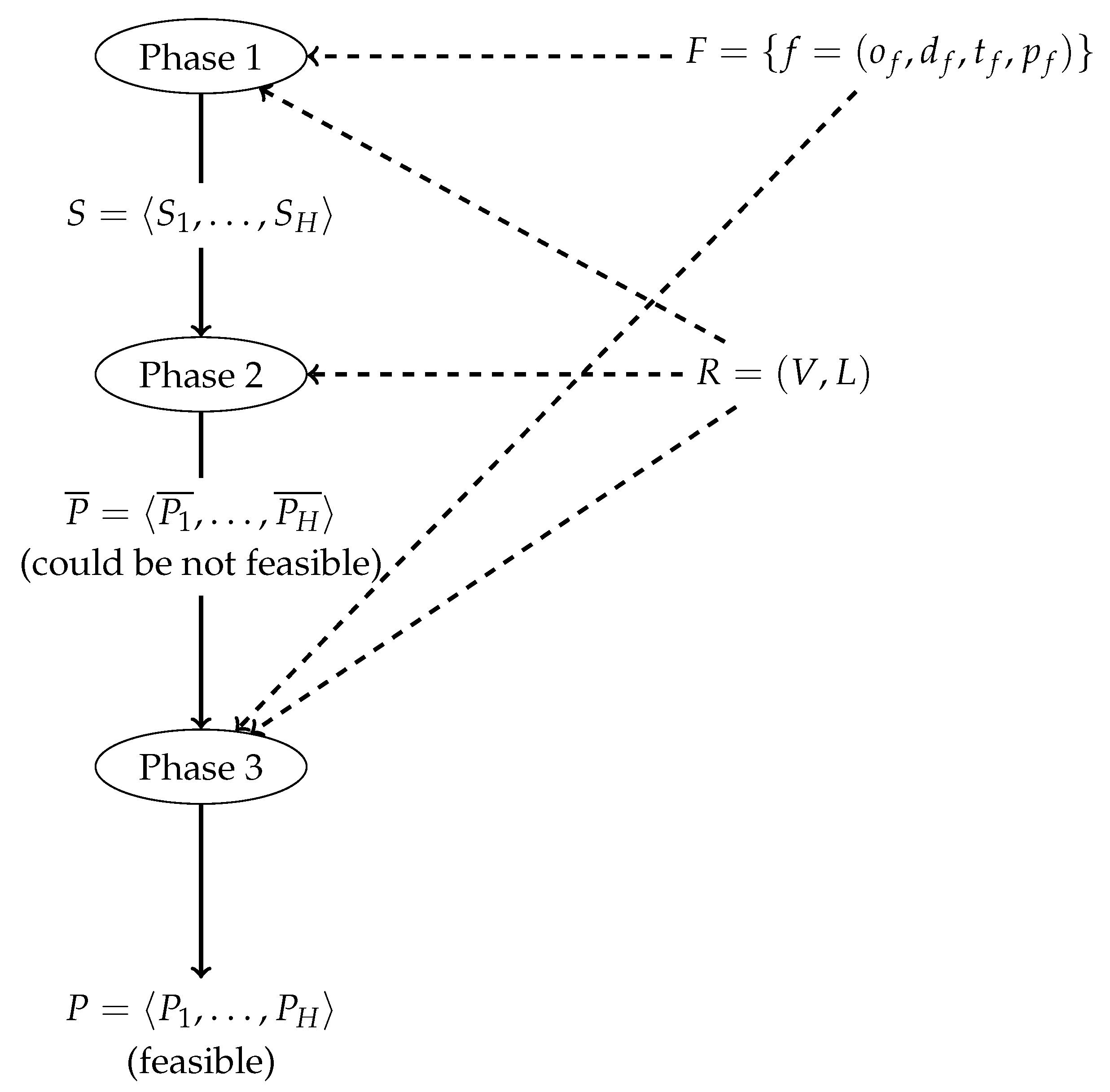
In the first phase, flows are time scheduled in each slot following an EDF approach as explained in Section 3. The output of this stage is a time schedule in which for every slot the flows that can be transmitted are listed. It is notated as $S=\langle S_1,\dots ,S_H\rangle$, where $S_h$, $1\le h\le H$, is the set of flows, as (source, destination) pairs, that the next stage will try to find a path in slot h.

The schedule obtained is used by the second phase in assigning available paths between source and destination while trying to keep the number of switches active as low as possible. In the second phase, flows may have different paths in each slot, and the path is not reserved for the whole flow duration. This means that a flow with a certain number of slot duration may be transmitted through different paths for each slot. This is similar to the routing of IP datagrams on the Internet in which each datagram may follow different paths. The paths are specified for each flow in each slot considering the energy demand in each case. This stage computes a schedule where some flows may have not been transmitted or some instances of them remain without being sent. This new schedule is notated with $\overline{P}=\langle \overline{P_1},\dots ,\overline{P_H}\rangle$, where $\overline{P_h}$ indicates the set of disjoint paths in R followed in slot h by the flows delivered in that slot.

The second phase searches paths for the flows scheduled in each slot but it does not control if each activation or flow is completely scheduled; therefore, the schedule might not be feasible for some flows or activations. This job is left to the third phase in which the schedule is revised. When an activation is not completely sent before its deadline, it is removed, and a different schedule is tried.

This means that first flows or activations are tried to be completely feasible. When this is not possible, the third phase eliminates completely the activation of flow from the whole schedule. If there are flows or activations that have not been scheduled previously, this last heuristic tries to schedule them. In this way, what the output of the third phase is a schedule of the system in which the flows or activations scheduled are completely transmitted.

In Figure 3, the diagram shows the interactions between the different stages that are explained in the next subsections.

5.1. First Phase: Time Schedule

In the standard fat-tree topology, each switch has the same number of inputs and outputs; therefore, in principle, every incoming flow will have an outgoing link. With these assumptions, the flows are parallelizable, that is, they can be transmitted simultaneously, as long as they do not share the same origin and/or destination. Based on this, two strategies were proposed for this first stage, where all the flows of the system are scheduled, giving priorities to those flows with the shortest period or nearest deadline.

Between the methods proposed for this stage, the first one consists of generating the scheduling for all the instances of each flow sorted from smallest to largest period. This fixed priority scheduling strategy ensures that flows with smaller periods are more likely to be transmitted. Algorithm 1 shows the pseudo-code of the procedure.

For the second alternative, whose pseudo-code is shown in Algorithm 2, the decision of which flow to send is performed on each slot of time, and flows are sorted from nearest to farthest deadline. This strategy has the advantage that it can be used as an on line scheduling policy, since the method performs a single pass and schedules only based on the deadline. The disadvantage is that, in the case of a periodic flow system, incomplete instances can occur for both low and high period flows.

The complexity of this heuristic is polynomial and is given mainly by the process of sorting the set of flows by deadline on every slot. For this reason, the complexity of the process is $\mathcal{O}(H\times |F|\times log|F\left|\right)$.

The output of this first stage is a list of flows to be allocated in paths for each slot ordered by priority. The priority is assigned according to periods or deadlines depending on the approach selected. If $\pi$ indicates the priority, when assigned by periods ${\pi }_j<{\pi }_i$ if $p_i<p_j$. This assignment is fixed and does not change with time, it is named Rate Monotonic. If priorities are related to deadlines, they are dynamic as the time remaining to reach a deadline decreases continuously. In this case, ${\pi }_j<{\pi }_i$ if $v_i<v_j$.

5.2. Second Phase: Maximum Edge Disjoint Path Problem (MEDPP)—Greedy Heuristics

In this second phase, three greedy heuristics are proposed. The output of the previous stage is divided in slots and considered independently. For each slot h, the set of flows to be allocated is maximized using the approach proposed in Maximum Edge Disjoint Path Problem (MEDPP) [38] but with the additional objective of minimizing the number of active switches or, equivalently, minimizing the energy demand.

Thus, when we compare two solutions for the MEDPP, we say the best one shall be the one with the most amount of flows allocated and the one that sends that quantity with the least energy consumption. Note that for this stage, a flow is defined by a pair origin-destination servers, unlike for the rest of the article where a flow also has associated a duration and a period.

Algorithm 1 First phase scheduling algorithm: first approach.
$h\leftarrow 0$	▹ Initialize the slot counter
$sort\_by\_period\left(F\right)$	▹ The set of flows is sorted by period
while $h<H$ do	▹ For each slot until reaching the end of the hyperperiod
for f in Fdo	▹ For each flow (starting from the one with lower period)
if $slots\_left\left[f\right]>0$ then	▹ If the current flow f is not transmitted
if $h>deadline\left[f\right]$ then	▹ If the current flow f is overdue
$reduce\_priority\left(f\right)$	▹ Reduce the priority of current flow
else	▹ If the current flow is still on schedule
if $feasible\left(f,h\right)$ then	▹ If it is feasible to transmit f in slot h
$allocate(f,h)$	▹ Allocate current flow to slot h
$slots\_left\left[f\right]\leftarrow slots\_left\left[f\right]-1$	▹ Reduce counter
end if
end if
else
if $h>deadline\left[f\right]-1$ then	▹ If it is the last slot for current instance
$slots\_left\left[f\right]\leftarrow size\left[f\right]$	▹ Update counter
$deadline\left[f\right]\leftarrow deadline\left[f\right]+period\left[f\right]$	▹ Update deadline slot
end if
end if
end if
$h\leftarrow h+1$	▹ Next slot
end while

Algorithm 2 First phase scheduling algorithm: second approach.
$sort\_by\_period\left(F\right)$	▹ The set of flows is sorted by period
for f in Fdo	▹ For each flow (starting from the one with lower period)
$inst\leftarrow 0$	▹ Initialize the instance counter
$h\leftarrow 0$	▹ Initialize the slot counter
while $inst<\frac{H}{p_f}$ do	▹ For each instance of current flow f
$left\leftarrow t_f$	▹ Number of slot left
$dl\leftarrow (inst+1)*p_f$	▹ Deadline of current instance
While $h<dlleft>0$ do	▹ While there are slots left and instance is not overdue
if $feasible\left(f,h\right)$ then	▹ If it is feasible to allocate flow f to slot h
$allocate(f,h)$	▹ Allocate
$left\leftarrow left-1$	▹ Decrease slot counter
end if
$h\leftarrow h+1$	▹ Next slot
end while
$inst\leftarrow inst+1$	▹ Next instance of flow f
$h\leftarrow dl+1$	▹ Next slot is the first of next period
end while
end for

The three heuristics use the $disjoint\_paths$ routine based on Breadth-first search algorithm to look for disjoint paths between source and destination servers. This routine, in addition to the network $R=(V,L)$, receives, as input, an ordered list S of pairs (source, destination) servers and returns a set of disjoint paths in R for as many pairs as possible.

It takes each pair (origin, destination) of servers from S following the order and, using $bfs\_shortest\_path$ routine, looks for a path C between them that uses as few switches as possible in the remaining network. If there is such a path, it marks the edges in C as used, blocking them for the other flows. The pseudo-code is shown in Algorithm 3, and its complexity is $\mathcal{O}\left(\right|S|*(\left|V\right|+\left|L\right|\left)\right)$.

Algorithm 3 disjoint_paths routine.

Require: Network R, a ordered list of pairs (source, destination) servers S

Ensure:$assign\_result$, set of disjoint paths in R between some pairs (source, destination) $\in S$

$remaining\_network\leftarrow R$

$assign\_result\leftarrow \varnothing$

for $(o,d)\in S$do

$C\leftarrow bfs\_shortest\_path(remaining\_network,o,d)$

if C is not empty then

$assign\_result\leftarrow assign\_result\cup C$

$remaining\_network\leftarrow remaining\_network-C$

end if

end for

return$assign\_result$

5.2.1. Simple

The first heuristic for this phase is shown in Algorithm 4. For each slot h, it takes the input set $S_h$ and orders it according to the priorities defined in phase 1. Then, apply the $disjoint\_paths$ routine on each of these ordered lists. The complexity of the simple heuristic is $\mathcal{O}({\sum }_{h\in H}|S_h|\times (log|S_h|+|V|+|L\left|\right))$.

Algorithm 4 Simple Greedy Heuristic.

Require: Network R, sequence of set of pairs (source, destination) servers $S=\langle S_1,\dots ,S_H\rangle$ with priorities

Ensure:$\overline{P}=\langle \overline{P_1},\dots ,\overline{P_H}\rangle$, where $\overline{P_h}$ indicates the set of disjoint paths in R followed in slot h by the flows delivered in that slot

$\overline{P}\leftarrow \langle \rangle$

for $h=1,\dots ,H$do

$S_o\leftarrow sort\_by\_priorities\left(S_h\right)$

$\overline{P}\leftarrow add\_back(disjoint\_paths(R,S_o))$

end for

return $\overline{P}$

5.2.2. Multistart

The second heuristic proposed in this phase is also greedy and can be seen in Algorithm 5. It consists in repeating the previous one several times permuting the order in $S_h$ randomly without repetition. From all the alternatives, the best solution is chosen. Through preliminary experimentation, it was observed that after 20 iterations the best solution rarely improves. Based on this, the $MAX\_ITER$ value was set at 20 for the following experiments.

5.2.3. Multistart-Adhoc

The last heuristic in this phase is presented in Algorithm 6. It is implemented in two steps. In the first one, a similar procedure to the Multistart one is used. In this case, the number of times that a flow $f=(source,destination)$ could be allocated is counted in $assigned\_count$. In the second step, the flows are ordered increasingly in relation to this value and a new simple heuristic is run to choose the best allocation between both steps, prioritizing flows that were assigned less frequently.

The idea behind this is that flows that are assigned less overall might have their few available paths taken by other so not restricted flows.

The worst running-time complexity is $\mathcal{O}({\sum }_{h\in H}|S_h|\times (log|S_h|+MAX\_ITERS\times (\left|V\right|+\left|L\right|\left)\right))$.

Algorithm 5 Multistart Greedy Heuristic.

Require: Network R, sequence of set of (source, destination) flows $S=\langle S_1,\dots ,S_H\rangle$ with priorities, $MAX\_ITERS\in \mathbb{N}$

Ensure:$\overline{P}=\langle \overline{P_1},\dots ,\overline{P_H}\rangle$, where $\overline{P_h}$ indicates the set of disjoint paths in R followed in slot h by the flows delivered in that slot

$\overline{P}\leftarrow \langle \rangle$

for $h=1,\dots ,H$do

$niters\leftarrow MAX\_ITERS$

$S\leftarrow sort\_by\_priorities\left(S_h\right)$

$best\_AR\leftarrow disjoint\_paths(R,S)$

while $niters>0$ do

$S\leftarrow shuffle\left(S_h\right)$

$assign\_result\leftarrow disjoint\_paths(R,S)$

if $assign\_result$ is better than $best\_AR$ then

$best\_AR\leftarrow assign\_result$

end if

$niters\leftarrow niters-1$

end while

$\overline{P}\leftarrow add\_back(best\_AR)$

end for

return $\overline{P}$

5.3. Third Phase: Feasibility Schedule

The second phase provides a schedule but depending on the approach or whole flows are left out in case they can not meet the deadlines or some activations of that flow are left out. In any case, flows or instances may be not fully sent. From a hard real-time point of view the system as a whole (all flows with all activations transmitted on time) is not feasible or at least a feasible solution considering all the flows and their activations were not found.

However, in soft real-time where some deadlines may be missed, the scheduling on time of as many flows or instances as possible, is important and constitutes a figure of merit of the system. In this last phase, flows are moved in search of enough space to add discarded flows or instances in a first round, and later a minimization of the used switches is done to reduce the energy cost. Algorithm 7 presents the pseudo-code for this phase.

This phase uses, as input, the set of paths found in the previous stage and attempts at first to complete those flows or activations that have not been completely scheduled. To do this, in the $make\_feasible$ procedure it uses the $bfs\_shortest\_path$ routine to search a path between source and destination through already used switches first. This is done in feasible or usable slots that have not been used by that flow/activation. If it is not possible to complete the flow/activation, it is removed and all paths and slots used are released. After this, a flow from those that has not been previously scheduled is chosen and allocated if possible ($improve$ procedure).

Finally, a certain number of iterations are made (this is an input parameter, $MAX\_ITERS$). In case this value is zero, the first solution is the one adopted. If it is higher, the solution is disturbed, and new allocations are tried.

Algorithm 6 Multistart Ad-Hoc Greedy Heuristic.

Require: Network R, sequence of set of (source, destination) flows $S=\langle S_1,\dots ,S_H\rangle$ with priorities, $MAX\_ITERS\in \mathbb{N}$

Ensure:$\overline{P}=\langle \overline{P_1},\dots ,\overline{P_H}\rangle$, where $\overline{P_h}$ indicates the set of disjoint paths in R followed in slot h by the flows delivered in that slot

$\overline{P}\leftarrow \langle \rangle$

for $h=1,\dots ,H$do

$niters\leftarrow MAX\_ITERS$

$assigned\_count\leftarrow \{f:0,f\in S_h\}$

$S\leftarrow sort\_by\_priorities\left(S_h\right)$

$best\_AR\leftarrow disjoint\_paths(R,S)$

while $niters>0$ do

$S\leftarrow shuffle\left(S_h\right)$

$assign\_result\leftarrow disjoint\_paths(R,S)$

if f is assigned in $assign\_result$ then

$assigned\_count\left[f\right]\leftarrow assigned\_count\left[f\right]+1$

end if

if $assign\_result$ is better than $best\_AR$ then

$best\_AR\leftarrow assign\_result$

end if

$niters\leftarrow niters-1$

end while

$S\leftarrow sort\_by\_assigned\_count\left(S_h\right)$

$assign\_result\leftarrow disjoint\_paths(R,S)$

if $assign\_result$ is better than $best\_AR$ then

$best\_AR\leftarrow assign\_result$

end if

$\overline{P}\leftarrow add\_back(best\_AR)$

end for

return $\overline{P}$

Algorithm 7 Third phase algorithm.

Require: Network R, set of flows F, $\overline{P}=\langle \overline{P_1},\dots ,\overline{P_H}\rangle$, where $\overline{P_h}$ indicates the set of disjoint paths in R followed in slot h by the flows delivered in that slot (could be not feasible), $MAX\_ITERS\in N$, $rRemove\in [0,1]$, $rInst\in [0,1]$, $rSlot\in [0,1]$, $nTries\in N$

Ensure: An feasible assignment of flows $P=\langle P_1,\dots ,P_H\rangle$, where $P_h$ indicates the set of disjoint paths in R followed in slot h by the flows delivered in that slot

$\overline{P}\leftarrow$ make_feasible($\overline{P}$)

$\overline{P}\leftarrow$ improve($\overline{P}$)

$P\leftarrow \overline{P}$

$niters\leftarrow MAX\_ITERS$

while $niters>0$do

$\overline{P}\leftarrow$ perturbation($\overline{P},rRemove,rInst,rSlot,nTries$)

$\overline{P}\leftarrow$ improve($\overline{P}$)

$niters\leftarrow niters-1$

if $\overline{P}$ is better than P then

$P\leftarrow \overline{P}$

end if

end while

return P

The $perturbation$ procedure first removes a certain percentage (given by the input parameter $rRemove$) of flows/instances. Then, the schedule is randomly modified by changing the slots and paths in which some flows are transmitted. This process is controlled by three input parameters.

The parameter $rInst$ indicates the percentage of instances to be considered, while $rSlot$ the percentage of slots or paths to be modified. Finally, $nTries$ sets the maximum number of slots in which a new path will be searched. If after $nTries$ attempts a path is not found in a new slot, the current slot and path are kept.

The pseudo-code for these procedures is omitted because of its simplicity. For routines $make\_feasible$ and $improve$, the worst running-time complexity is $\mathcal{O}\left(\right|F|\times H\times (\left|V\right|+\left|L\right|\left)\right)$, while for the $perturbation$ routine it is $\mathcal{O}(rInst\times rSlot\times nTries\times |F|\times H\times (\left|V\right|+\left|L\right|\left)\right)$. This results in a computational complexity of Algorithm 7 of $\mathcal{O}\left(\right(\left|F\right|\times H\times \left(\right|V|+|L\left|\right))\times (1+MAX\_ITERS\times (rInst\times rSlot\times nTries+1))$.

As there are many tuning parameters for this third phase, the toolbox IRACE [39] is used to optimize them.

6. Experimental Evaluation

In this section, several experiments with the different heuristic approaches are presented and compared for synthetic sets of problems with different characteristics. The experiments were carried out on a personal computer with Ubuntu Server 20.04 with processor Intel I7-10700 running at 2.9 GHz and 64 GB of RAM. All the implementations are written in the C++ programming language.

As mentioned in previous sections, flows are periodic with real-time constraints. It is enough to evaluate the behaviour of the system up to the hyperperiod (H), which is given by the least common multiple of all the periods. As the system schedules for each slot the flows to be transmitted and their allocation to different paths, the size of the problem to be solved is proportional to the amount of servers, network switches, links, flows and the hyperperiod. In the evaluation, the periods were selected to set H to 300 slots in order to keep the simulation time at reasonable values. This is a discretionary value that has no real impact in the comparison metric but does in the time necessary to compute the solutions.

It is assumed that switches can be turned on and off on demand and that all of them have identical electrical characteristics and can process flows at the same speed. In this scenario, it is sufficient to compare how many elements are active at each slot. The worst case, or maximum energy demand, is given if during the whole hyperperiod all elements are active. In case there are less elements active, those without traffic can be turned off and with this during that slot some energy is saved.

In a fat-tree topology, the number of switches is a function of the number of servers. When all switches are active the energy demand of the infrastructure during the hyperperiod is considered nominal, $E_{\mathrm{nom}}$, and its value is used as reference to compute the savings. In the same way, once the scheduling of flows have been computed, only the active switches in each slot demand energy and the actual energy consumed by the infrastructure during the hyperperiod can be computed, $E_{\mathrm{consumed}}$. The relation between both values represents the energy saved; see Equation (15).

$$Saving=100(1-\frac{E_{\mathrm{consumed}}}{E_{\mathrm{nom}}})$$

(15)

However, this value has to be normalized to be useful in comparisons. When the system schedules only a few flows or activations, only a subset of the switches would be active and the rest of the infrastructure can be turned off. The normalization is done by incorporating, in Equation (15), the relation between the number of scheduled flows to the total number of flows when the scheduling is done based on flows or the relation between activations when it is done per activation.

$$\begin{array}{cc}\hfill N\_Saving\_F& =Saving\frac{\mathrm{Flows}\_\mathrm{Scheduled}}{\mathrm{Total}\_\mathrm{Flows}}\hfill \\ \hfill N\_Saving\_A& =Saving\frac{\mathrm{Act}\_\mathrm{Schedules}}{\mathrm{Total}\_\mathrm{Act}}\hfill \end{array}$$

(16)

As mentioned in Section 5, the IRACE package, for automatic configuration of optimization algorithms [39], was used to tune the input parameters of the algorithms. The experiments were performed with several sets of instances. Systems with 8, 16, 32, 64 and 12eight servers were generated in fat-tree DCN topologies. For each set different amounts of flows were simulated with bandwidth demands between 0.2 and 1 for each server. Results are presented only for 8 and 12eight servers as they represent the most significant cases.

To avoid increasing the complexity of the tuning task, the domain of some parameters was restricted to the most relevant values.

Table 3. Configuration of input parameters.

Parameter	Domain	Best Value Flows	Best Value Activations
First phase approach	1, 2	1	2
$rRemove$	0, 0.1, 0.5	0	0
$rInst$	0.3, 0.5, 0.8, 1	0.3	0.3
$rSlot$	0.3, 0.5, 0.8, 1	0.3	0.5
$nTries$	10, 30, 50	10	10

shows the domain considered for each parameter and the best value reported by IRACE.

Clearly, by increasing the number of iterations both in the Multistart algorithm of phase 2 and in the perturbation and improvement procedure of phase 3, the solution obtained will be better, since both procedures return the best solution found. Clearly, by increasing the number of iterations in the perturbation and improvement procedures of phase 3, the solution obtained will be better, since the procedure returns the best solution found. A similar situation happens with the different heuristics proposed for phase 2.

The Simple heuristic will be faster, but the solution obtained with the Multistart Ad-Hoc will be of better quality. Therefore, for these parameters, an analysis of the compromise between the quality of the solution found and the execution time will be made later. The column “Best value Flows” refers to the best parameter setting for the version where the sending unit is the complete flow, and the column “Best value Instances” for which it considers an instance as a unit.

The first parameter listed is the one that selects the approach in phase 1. This first stage is important as its output is a time scheduled for each slot. In the first approach, the scheduling unit is the flow while in the second it is the activation of the flow. In the first case, the algorithms order the queue of pending flows to be sent by the period while in the second it uses the deadline. It is natural then that, when in the following stages, the scheduling is based on the activations, the best option for the first phase is the second approach.

As can be seen in the Table 3, in the perturbation procedure in phase 3, in neither of the two approaches it is convenient to delete flows or activations that are being sent to try to make room for others. Furthermore, the best performance is obtained when the percentage of instances and slots to be moved is low. This indicates that the decisions made in the previous phases are adequate and it is not convenient to undo them. It is only useful to make small movements in terms of slot or path used. On the other hand, at higher values of $nTries$, the improvements obtained in the quality of the solutions are negligible or null, and thus the cost in execution time that this requires does not make sense, and with a value of 10 the best performance was obtained. These configurations are kept for the next experiments.

In all the tables that follow, the “Flows/Act columns” represent the number of flows or activations sent in the solution found by the respective algorithm. The “N_Saving_F” or “N_Saving_A” column is computed according to Equation (16). To some extent, this considers the effectiveness of the solution with respect to the two objectives, number of flows or activations sent and energy consumption. For heuristics, the Time column expresses the time taken by each one in seconds.

Validation of the Methodology

This first experiment has the purpose of validating the methodology. Although it is not possible to assert that the behaviour with small cases is similar to that with big systems, it provides an idea of the different speeds and quality of the results in finding a solution.

In the first place, small systems were defined in order to obtain solutions from the ILP formulation and compare them with those obtained with the heuristics. To solve the ILP model, CPLEX v20.1.0 was run with the default parameters (https://www.ibm.com/docs/en/icos/20.1.0, accessed on 15 February 2022) for a maximum of 1800 [s] using all the computing power of the server for each of the objectives, first to maximize the number of flows or activations sent, and then to minimize the cost power (number of total switches turned on per slot).

Five different sets of flows or problem instances were generated in a random way for a system with eight servers and 10 switches. Each instance has 30 flows to be scheduled between the different servers. The utilization factors for all them were set to 1.6, 3.2, 4.8, 6.4 and 8. As a uniform distribution was used for the generation of the flows, on average, this means that each server has a bandwidth demand of 0.2, 0.4, 0.6, 0.8 and 1.

The interferences between flows from different source servers in the same destination server can produce priority inversions causing deadline misses on one hand and on the other, as it is a random generation, some servers may be overloaded. Both things make that the systems generated may not be able to schedule all the flows on time. It is for this that, in the experiments, the percentage of successfully scheduled flows is considered together with the energy saving in the networks as a figure of merit.

In

Table 4. Eight servers-30 flows-Flow scheduling with Simple heuristics in phase.

	ILP (1800 [s])		${\displaystyle \mathit{MAX}\_\mathit{ITER}=0}$			$\mathit{MAX}\_\mathit{ITER}=20$			$\mathit{MAX}\_\mathit{ITER}=50$
U	Flows	N_Saving_F	Flows	N_Saving_F	Time	Flows	N_Saving_F	Time	Flows	N_Saving_F	Time
0.2	30	87.01	30	83.84	0.05	30	83.84	0.06	30	83.84	0.07
0.4	30	73.13	30	69.17	0.09	30	69.17	0.11	30	69.17	0.15
0.6	27.40	58.38	25.20	52.15	0.13	25.60	51.89	0.20	25.60	51.90	0.29
0.8	25	49.29	23.80	45.57	0.15	24.20	45.79	0.22	24.20	45.87	0.33
1	21	41.79	18.60	36.82	0.16	19.20	37.23	0.27	19.20	37.25	0.43

and

Table 5. Eight servers-30 flows-Activation scheduling—Phase 2 Simple.

		ILP (1800 [s])		$\mathit{MAX}\_\mathit{ITER}=0$			${\displaystyle \mathit{MAX}\_\mathit{ITER}=20}$			${\displaystyle \mathit{MAX}\_\mathit{ITER}=50}$
U	Total Act	Act	N_Saving_A	Act	N_Saving_A	Time	Act	N_Saving_A	Time	Act	N_Saving_A	Time
0.2	72.20	72.20	87.00	72.20	83.76	0.05	72.20	83.76	0.06	72.20	83.76	0.09
0.4	76.40	76.40	73.41	76.40	68.95	0.09	76.40	68.95	0.13	76.40	68.95	0.19
0.6	70.60	66.80	60.36	65	56.92	0.13	65.60	56.28	0.22	65.60	56.30	0.35
0.8	75.40	67.60	52.18	65.80	50.06	0.15	66.80	49.61	0.27	66.80	49.62	0.43
1	72.60	58.80	45.69	53.80	43.31	0.16	55	43.40	0.33	55	43.45	0.58

, the results are presented for this first set of instances for the case in which the scheduling is made per flows and per activations, respectively. In the first section of the table, the result obtained with CPLEX with the ILP model is shown. Even for a small system like this, with only a few servers and flows, the exact solution is not obtained within the time limit. However, as CPLEX provides additional information, such as upper and lower bounds, we know that there is a solution and that the actual gap to the optimal value is not large.

In the case of maximizing the amount of flows, a solution is found fast when $U<1$. However, for $U=1$, it can not find an optimal solution in 1800 [s]. The result presented in Table 4 is the best value obtained up to that instant. In the case of maximizing the amount of activations, the solver can not find an optimal solution in 1800 [s] when $U>0.6$. As before, the results presented in Table 5 are the best values.

With respect to the second objective, minimizing the energy demand, neither approach finds an optimal solution within 1800 [s]. The results shown are then the best values obtained within that time limit. In the following columns, the results obtained with the Simple proposed heuristic for the second stage are presented for the cases in which, in the last phase, 0, 20 or 50 iterations are performed trying to improve the result obtained.

This first experiment shows several important issues. In the case of scheduling flows, as the utilization factor increases to 1 for the servers, there is a reduction in the number of feasible flows and an important reduction in the savings obtained. Both things are within the expected response of the model. As explained in Section 3, there may be interference between flows in different servers because they share the same destination, and this eventually produces a priority inversion that makes the flow not schedulable.

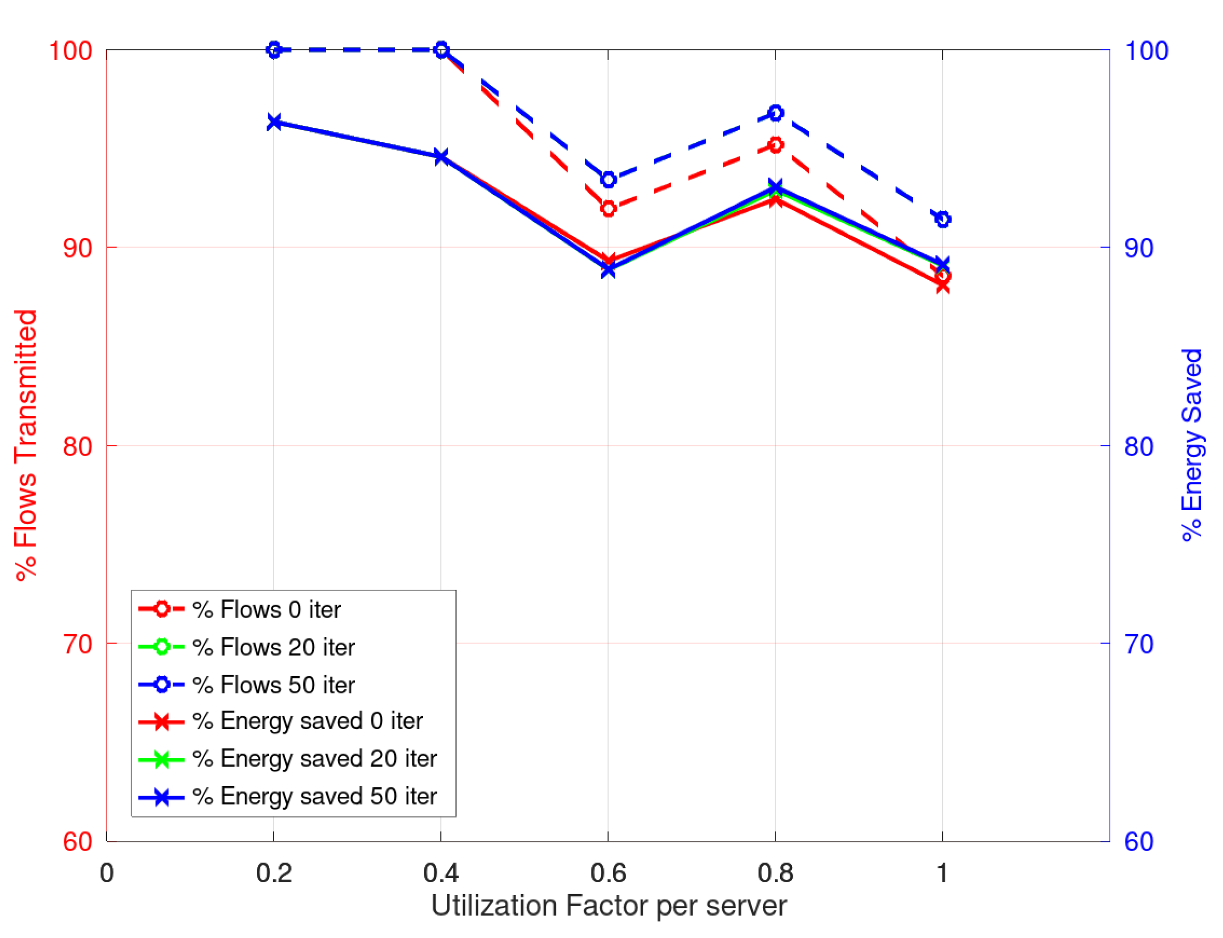
Considering the solution obtained by CPLEX as benchmark we can see that the results obtained with the heuristics with 0, 20 or 50 iterations in the third phase, are quite similar. In Figure 4, the relative results are presented. As can be seen, the response of the heuristic in its different versions is good. On the left axis, the percentage of scheduled flows is shown with respect to the CPLEX solution, and on the right axis the energy saved with respect to the CPLEX solution. The results show that the heuristic results are within 90% of the ones obtained with the CPLEX solver but they demand about four orders of magnitude less execution time.

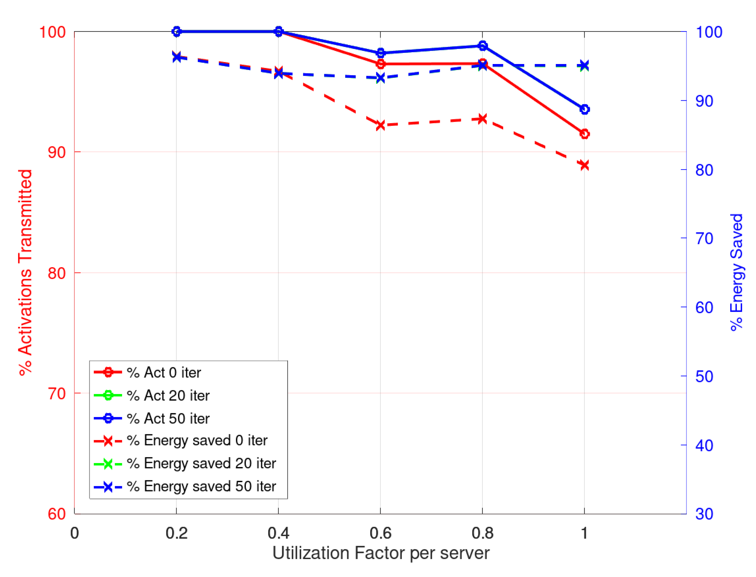
When considering the scheduling by activations, CPLEX finds a solution for the first objective for the lowest utilization factors, 0.2 and 0.4, but—as in the case of flows—no optimal solution is reached for the minimization of energy demand within the time limit of 1800 [s]. However, the heuristic can solve the problem in all cases with less than a second computation. Figure 5 shows the results and, as in the previous case, the CPLEX results are taken as a reference. The percentage of energy saving is in the right axis and the percentage of activations scheduled is on the left one.

When reading the results, it may appear contradictory that with more iterations in the final phase the heuristic presents less energy savings when the utilization factor increases. However, the reader should pay attention to the fact that, for both approaches, flows or activations, when more iterations are done in the final phase, a higher percentage of flows or activations are scheduled. This clearly increases the energy demand.

In Figure 5, it may appear that the energy saving improves greatly with higher utilization factors. This result can be explained as what is shown is the relation to the CPLEX values and as explained before, the solver was not able to find a good solution within the time limit. This clearly leaves the CPLEX value more close to the heuristic solution found.

A more complex system was simulated based on the good results obtained in this first experiment. As before, five instances for a system with 12eight servers and 1000 flows were randomly generated following the same method for each utilization factor. The ILP model in CPLEX was impossible to run as the number of variables was too large even for a 64GB RAM machine. The results are presented in

Table 6. 12eight servers-1000 flows-Flow scheduling with Simple heuristic in phase 2.

	${\displaystyle \mathit{MAX}\_\mathit{ITER}=0}$			${\displaystyle \mathit{MAX}\_\mathit{ITER}=20}$			${\displaystyle \mathit{MAX}\_\mathit{ITER}=50}$
U	Flows	N_Saving_F	Time	Flows	N_Saving_F	Time	Flows	N_Saving_F	Time
0.2	999.40	66.09	0.32	1000	64.38	1.96	1000	64.38	4.43
0.4	982.60	35.33	0.61	999.60	23.29	4.97	999.60	23.29	11.61
0.6	936	15.14	1.09	956.40	9.67	8.83	957.60	9.64	19.63
0.8	812.25	6.86	1.85	821.25	5.30	13.77	821.25	5.53	25.60
1	672.67	4.90	2.63	678.33	4.00	19.50	678.33	4.17	34.77

,

Table 7. 12eight servers-1000 flows-Flow scheduling—Phase 2 Multistart Ad-Hoc.

	${\displaystyle \mathit{MAX}\_\mathit{ITER}=0}$			${\displaystyle \mathit{MAX}\_\mathit{ITER}=20}$			${\displaystyle \mathit{MAX}\_\mathit{ITER}=50}$
U	Flows	N_Saving_F	Time	Flows	N_Saving_F	Time	Flows	N_Saving_F	Time
0.2	1000	66.33	4.19	1000	66.33	5.82	1000	66.33	8.29
0.4	988.20	35.49	8.34	999.60	24.00	12.65	999.60	24.00	19.25
0.6	948.80	15.25	11.89	960.60	9.93	19.45	961.20	9.81	30.15
0.8	822.80	6.68	14.56	829.40	5.20	26.46	829.60	5.44	37.90
1	682	4.70	16.09	684.20	4.10	33.48	684.20	4.21	49.27

,

Table 8. 12eight servers-1000 flows-Activation scheduling—Phase 2 Simple.

		${\displaystyle \mathit{MAX}\_\mathit{ITER}=0}$			${\displaystyle \mathit{MAX}\_\mathit{ITER}=20}$			${\displaystyle \mathit{MAX}\_\mathit{ITER}=50}$
U	# Act	Act	N_Saving_A	Time	Act	N_Saving_A	Time	Act	N_Saving_A	Time
0.2	2477.40	2476.80	66.02	0.29	2477.40	66.19	3.37	2477.40	66.19	7.99
0.4	2517.20	2505	35.21	0.57	2516.80	23.40	8.59	2516.80	23.40	20.70
0.6	2511.60	2443.40	15.17	1.04	2467	9.72	13.62	2467.60	9.82	30.20
0.8	2520.80	2266	6.74	1.82	2293.80	5.15	18.23	2294	5.37	32.15
1	2507.20	2019.80	5.17	2.54	2040	4.10	25.52	2040.20	4.32	44.35

and

Table 9. 12eight servers-1000 flows-Activation scheduling—Phase 2 Multistart Ad-Hoc.

		Constructive			20 Iterations			50 Iterations
U	# Act	Act	N_Saving_A	Time	Act	N_Saving_A	Time	Act	N_Saving_A	Time
0.2	2477.40	2477.40	66.21	4.18	2477.40	66.21	7.28	2477.40	66.21	11.90
0.4	2517.20	2504.8	35.34	8.34	2516.8	23.51	16.37	2516.80	23.51	28.49
0.6	2511.60	2452	15.25	11.95	2467	9.81	24.54	2467.60	9.92	41.12
0.8	2520.80	2285	6.77	14.88	2293.8	5.21	31.28	2294	5.43	45.20
1	2507.20	2032.60	5.09	16.13	2040	4.14	39.01	2040.20	4.37	57.84

, for the cases of using the Simple or Multistart Ad-Hoc for the second stage with flow or activations scheduling, respectively. Multistart results are not presented as they are part of the Ad-Hoc implementation, which improves the solutions found.

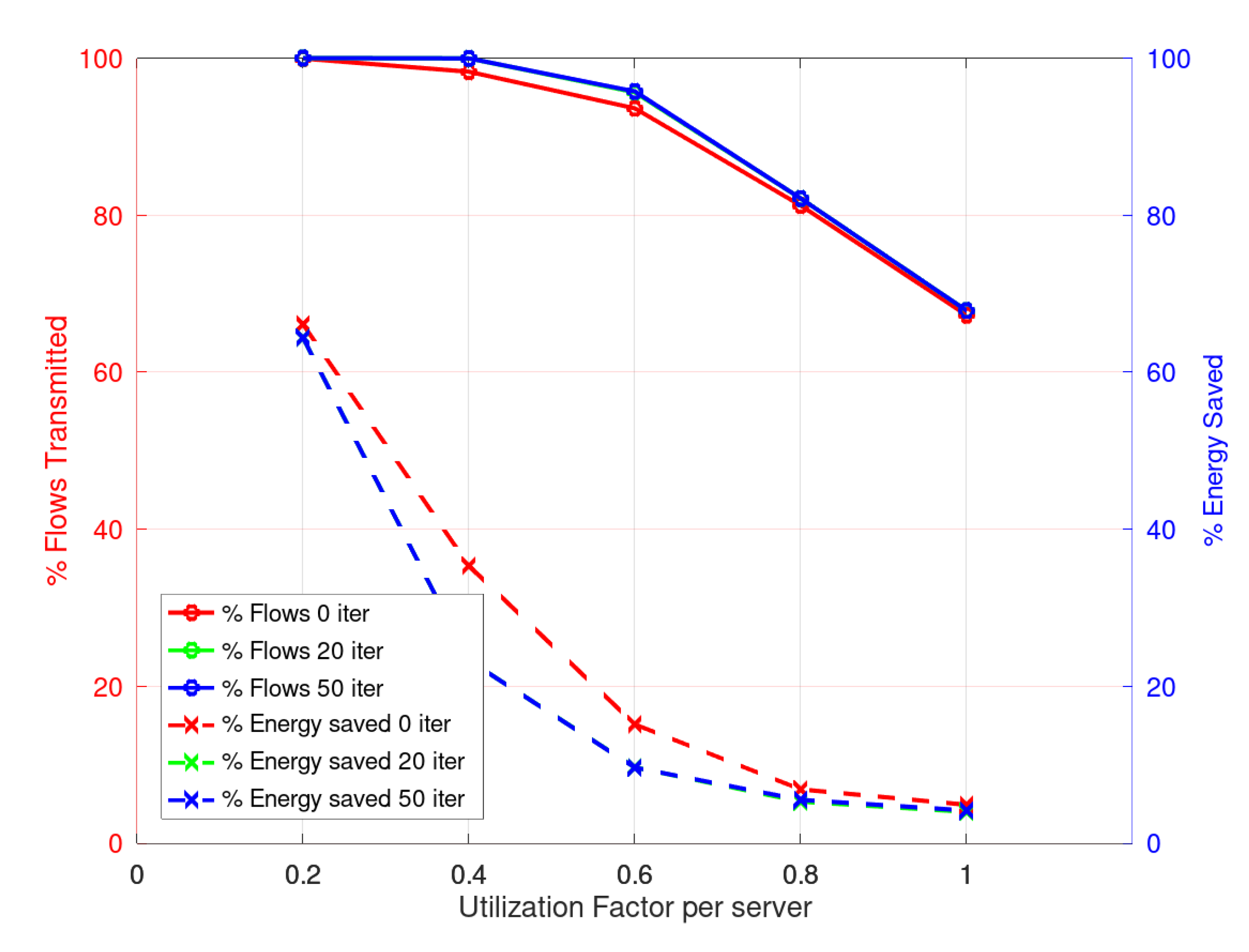
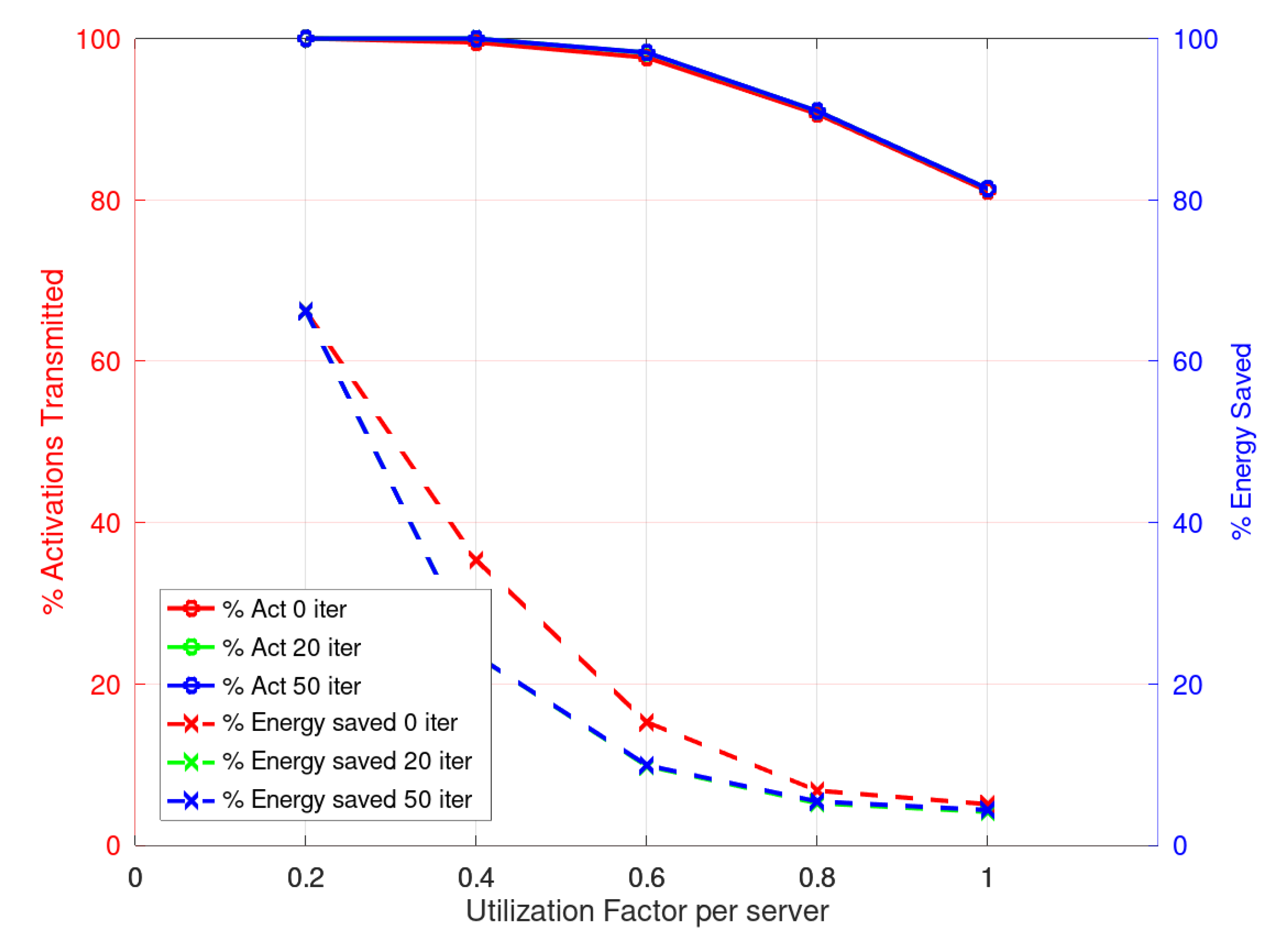
In these cases, the relation is made to the nominal system as it was not possible to run the CPLEX solver. Figure 6 presents the results for the Simple heuristic with the flow scheduling approach. This shows, on the left axis, the percentage of energy saved with respect to all the network elements active and, on the right axis, the percentage of flows scheduled. As can be seen, although the energy saved is less when more iterations are made in the third phase, there is an increase in the number of flows scheduled. However, there is no significant improvement in doing 50 iterations compared to only 20, while there is an important increase in the computation time.

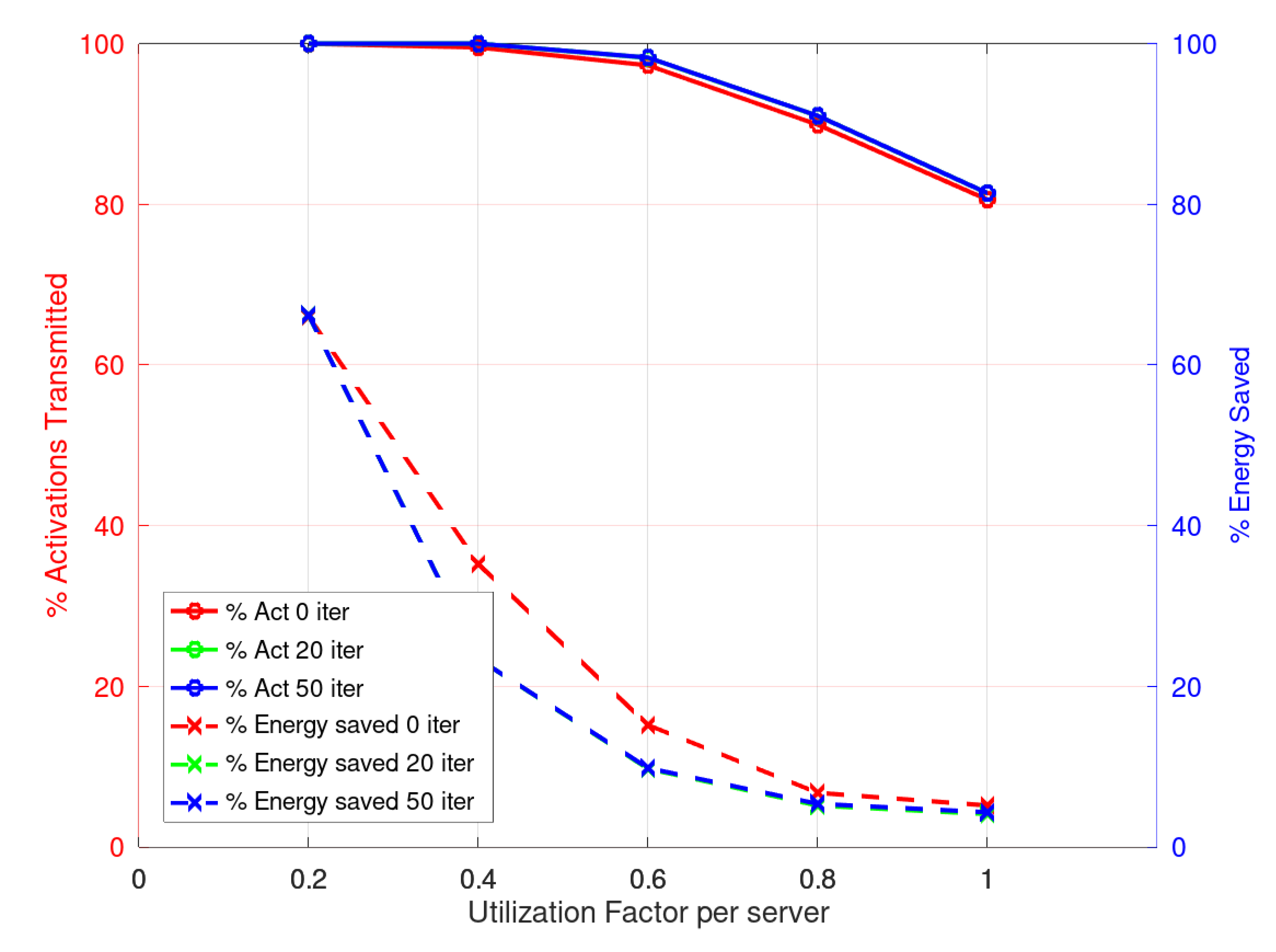
Figure 7 presents the results for the Simple heuristic with the activation scheduling approach. It shows, on the left axis, the percentage of energy saved with respect to all the network elements active and, on the right axis, the percentage of activations scheduled.

As can be seen, although the energy saved is less when more iterations are made in the third phase, there is an increase in the number of activations scheduled. However, there is no significant improvement in doing 50 iterations compared to only 20, while there is an important increase in the computation time of about 50%.

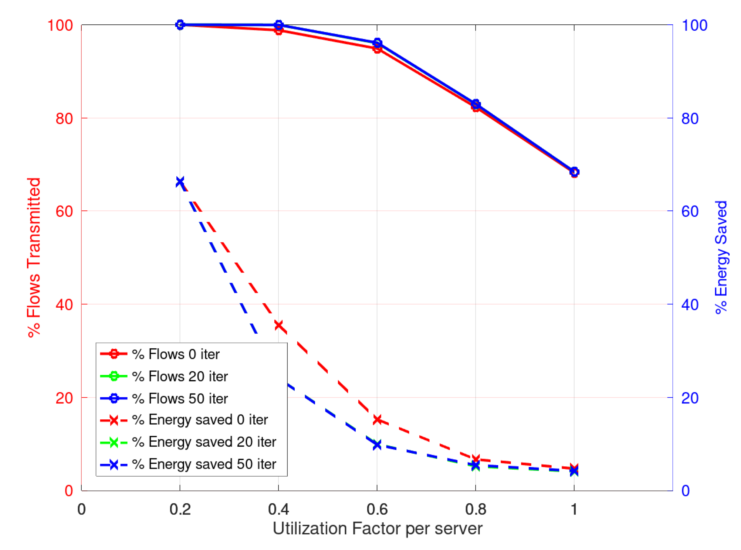
Figure 8 and Figure 9 present the results for the Multistart Ad-Hoc heuristic in phase 2. It is important to notice here that the amount of flows or activations that are scheduled is larger than that obtained with the Simple heuristic. Although the time required is larger, the possibility of scheduling more flows or activations is important as it is a figure of merit of the system. Clearly, the amount of energy saved in these cases is lower; however, this is related to the fact that the network is busy for a longer time.

7. Discussion

The experimental results presented in the previous section show the complexity of the problem we are attempting to solve. The first aspect to mention is that the ILP model and its exact solution through solvers, like CPLEX, is not possible in a reasonable time when the problem grows in some of its variables. The second aspect to mention is that the heuristics used, although they are really simple, provide good results. There is a trade off between the complexity of the heuristic and the time required to find a schedule. The results show that, with more iterations in the second and third phases, more flows or activations can be feasible.

Clearly, this implies more energy demand. However, the main objective of the optimization process is to send as many flows or activations as possible consuming as less energy as possible; however, the second objective is a subsidiary of the first. The best results are obtained with Multistart Ad-Hoc and 50 iterations in the last phase. However, with 20 iterations, the results are similar, less than 1% improvement, and they are obtained in about two thirds of the time. In general, in the figures it is not possible to discriminate between the results obtained with 20 or 50 iterations; thus, it is reasonable to think that it is enough to perform up to 20 iterations in the last phase.

With high bandwidth demands to the servers, from 0.8 to 1, not all flows or activations can be scheduled on time. This is related to the interference that flows imposed within destination servers that produce priority inversions at the source servers. In relation to the energy saving, with high utilization factors and a large amount of flows to schedule, there is as much as 5% saving. This is a consequence of the need to use all possible paths to transmit the flows on time. With a few servers and flows, the energy saving is more significant; however, in this case, the flows have a large duty-cycle but likely require less paths.

The computation time of the schedule is a key issue. The benefits of doing a proper schedule with energy saving have to be measured in relation to the delay in beginning the processing demand by servers. The use of this kind of policies can be applied when the dynamic of the system is such that setting the paths in the DCN represents a small amount of the time the system will operate in that configuration.

Considering a 30 [s] computation time for 1000 flows between 12eight servers, this implies for 10% overload in scheduling, dynamics of 300 [s] or five minutes, and with 1% overload, dynamics of 3000 [s] or fifty minutes. In the case that the system does not change its demand for five minutes, the cost of scheduling the flows is about 10%; however, if the time is extended to fifty minutes, the cost of scheduling the system is about 1%, which is quite reasonable.

Becoming Real

The use of DCNs is common today in management areas within governments, banks, universities, military, business and health systems, among others. They rely on the operation of networks of servers where all the information is stored. Different requirements are associated, such as security, availability, reliability, latency and, most importantly, the costs of implementation and maintenance.

The latter are key because there is a trade off between hosting a DCN in an appropriate building or hiring the service from a dedicated company, for example Google, Amazon or Microsoft, to mention the most common ones. These companies usually provide the service to clients with different plans according to their requirements. In some cases, they rent all the hardware involved (servers and switches) to be managed by the clients, or provide a virtual DCN, in which case, servers and switches may be physical or virtual machines or they could provide the whole service with both hardware and software. In all cases, DCN hosting business is constantly evolving [4,5].

The international standard ISO22237 [40] provides a taxonomy based on the facilities and infrastructure of the DCNs. Essentially, four different types of DCN are defined according to their complexity. The first level is a single path solution, which is the most simple. The second category provides a path with a redundancy solution. In the third level, there is multi-path access together with the option to repair and operate the centre in a concurrent way. The last one provides a multi path-solution together with fault tolerance. As the complexity of the DCN increases, the amount of servers providing backup of the information is also increased.

DCNs require different aspects to be taken into account when mounted. The building infrastructure, the cooling system, the network components, the servers and power supplies. Companies are reluctant to provide information on the actual sizes of their DCN; however, there are indications based on the power consumption of the building and their overall dimensions. The trade off of implementing a local DCN or hosting it with some provider is out of the scope of this paper.

In this section, results for a DCN with 8192 servers and 10,000 flows are presented. To solve this in a reasonable period of time and using the simplest version of stage 2, two algorithms were implemented, limiting phase 3 to simple procedures. In the first one (ALG 1), only incomplete flows or activations were removed from the schedule. In the second one (ALG 2), the original make_feasible routine is executed, which attempts to complete a flow or activation before removing it.

The time needed to achieve a possible schedule is substantial, and the computer on which the algorithm is implemented may require large computing resources. If the heuristic is adapted to run on a GPU or using a multithreaded approach, the execution time could be reduced. In large DCNs, the servers typically have powerful processors, and it seems likely that the heuristic could be executed within a reasonable time. The results are presented in

Table 10. 8192 servers-10,000 flows-Flow scheduling with simple heuristics in phase 2.

	ALG 1			ALG 2
U	Flows	N_Saving_F	Time	Flows	N_Saving_F	Time
0.2	9956.00	61.85	686.42	9960.40	62.01	700.76
0.4	7928.00	31.85	1195.02	8271.60	35.43	1724.03
0.6	5715.60	18.40	1417.64	6272.80	23.03	2543.02
0.8	3916.20	12.52	1422.73	4477.60	17.89	3064.09
1	3584.20	10.01	1540.72	4382.80	13.43	3514.58

and

Table 11. 8192 servers-10,000 flows-Activation scheduling with Simple heuristic in phase 2.

		ALG 1			ALG 2
U	# Act	Act	N_Saving_A	Time	Act	N_Saving_A	Time
0.2	24960.00	24914.00	61.96	685.80	24915.20	62.10	698.79
0.4	25033.40	22252.40	34.11	1243.09	22587.60	37.10	1715.35
0.6	24970.80	18468.40	21.18	1523.18	18979.00	25.20	2485.95
0.8	25091.00	13277.40	13.21	1648.33	13419.40	21.67	3142.50
1	25022.00	13206.40	11.74	1740.84	13337.40	16.22	3303.28

.

As presented in the previous experiments, scheduling was performed on a per flow basis. The results obtained are also consistent when tested on smaller systems. Basically, there is an important energy saving at low utilization factors ($U=0.2$, saving over 60%) but it is reduced when there is more network demand ($U=0.8$, saving above 10%). Another aspect that is worth mentioning is that there is an important loss in the amount of flows or activations being scheduled when the utilization factor increases close to 100%.

As expected, the computational complexity of the implemented heuristics strongly depends on the parameters of the system to be scheduled, but in all cases it is polynomial. Depending on the approach chosen in the second and third phases, the complexity may be higher or lower overall. In the first phase the complexity is a function of the number of flows to be scheduled per the hyperperiod, while in the second phase using the Simple option again the hyperperiod is present together with the size of the fat-tree under study, amount of nodes and links. Finally, the simplest form of the third phase depends again on the hyperperiod, the size of the fat-tree and the number of flows or activations. Therefore, the overall complexity is polynomial.

8. Conclusions and Future Work

In the present work, the time and path scheduling of real-time flows in DCNs was modelled and implemented using an ILP exact resolution model and through ad hoc heuristics. The problem is NP-hard, and the ILP model can not scale up when the number of servers and/or flows grows from only a few. The proposed heuristic approach consists in dividing the scheduling algorithm into three phases. In the first phase, the flow activation slots were defined using well-known scheduling policies, such as EDF or RM. In the second phase, the choice of path was performed in each slot for each flow. Finally, in the third phase, the schedule was revised and incomplete flows or activations were scheduled, when possible, or completely removed in order to gain time slots for previously left out flows/activations.

Our results show that the scheduling and path selection problems can be solved simultaneously by means of the proposed heuristics in a short period of time with the advantage of reducing the energy demand of the network infrastructure while satisfying the real-time requirements. Different alternatives consisting of simple heuristics were provided that showed good overall performance. The solutions obtained by means of the proposed heuristics improved in terms of quality as more iterations were performed; however, they did so at the expense of increasing the computation time. For a first-path solution, the best results were not far from those obtained with a higher number of iterations, which shows that, depending on the generated flows on the network, a system administrator can choose between different scheduling approaches.

As future work, an attempt will be made to analyse different solutions when the size of the DCN is scaled up to thousands of servers and including different DCN topologies. For this case, the possibility of dividing the network into subnetworks will be considered, as one of the main challenges of the proposed approach relies on the memory usage of the optimization algorithms.