1. Introduction
The Internet is slowly moving and migrating from the Internet of people to the Internet of things. Internet of things (IoT) devices can become pervasive and enable context-aware and environmental intelligence [
1,
2]. However, the ability to interact between heterogeneous Internet objects, mobile handheld devices, and wireless sensors faces severe complications [
3]. A network of sensors contains self-organizing networks made up of several nodes dispersed across an area that gather the necessary data and transmit them to a base station node [
4]. Sensors are crucial parts of intelligent things. One or more sensors are necessary for all IoT applications to gather environmental data. Receiving information, which is essential to the IoT, is only feasible with sensing devices.
Internet of things sensors are primarily tiny, low-power, and low-cost, limited by features such as their ease of deployment and battery capacity [
5]. In this research, the focus is on integrating sensor networks and the Internet of things, as well as detecting outlier sensors [
6]. However, the development of the Internet of things faces several obstacles. These difficulties are social and professional. These obstacles need to be cleared away to guarantee the adoption and penetration of the Internet of things.
The location and proper communication of sensors are essential in sensor-based computer networks to perform optimal tasks. In addition, location information is helpful in geographic routing and joint signal processing [
7]. Using different methods, researchers try to choose the best location for sensors so that service delivery in sensor-based networks can be adequately carried out [
8].
One of the suitable approaches to removing network outlier sensors is the use of location knowledge. However, in the meantime, a sensor or sensors with incorrect placement may challenge the network [
9].
Such sensors will be called outlier sensors in this article. Location is the best place to establish service providers’ facilities, and they are also trying to reduce lost demand by rationally allocating the demand centers to them. Sensor positioning is also a subset of these issues [
10].
The placement of sensors in sensor-based networks seems impractical due to the nature of such networks; in addition to many sensors, their position is inaccessible in some applications [
11]. Although the global locating system may be utilized to determine the location of sensors, its use is not always possible, in addition to it being expensive [
12]. Therefore, alternative methods should be used.
The Internet of things is a subset of computer networks that have recently gained popularity. In this network, a set of sensors is placed in a defined workspace, providing services by establishing communication [
13]. In the meantime, a sensor with a lousy placement may challenge the network.
Technological advances in low-power integrated circuits have made it possible to build low-cost as well as small-sized sensor nodes and create wireless sensor networks by connecting them. Sensor nodes can sense, process, and send data [
14]. The significant discrepancy between communication networks and these sensor networks is their data-centric nature and minimal energy as well as processing resources.
In a sensor network, many small nodes autonomously monitor and interact with the environment. These sensors take information from the environment and transfer it to a data collection center [
15]. One of the characteristics of these sensors is independence and operation without human intervention. Sensors can be used in small spaces due to their small size and limited memory, processing power, and battery. Since there is no base station in wireless sensor networks and their radio frequency is low, the dispersion of nodes should be such that the nodes are in each other’s radio coverage and deliver the sensed data to the destination from the nearest route while thoroughly covering the area. Usually, due to the geographical location of these types of networks in dangerous environments and the remote locations of some nodes, it is impossible to recharge or use them properly [
16]. Therefore, choosing the correct location of sensors and removing extraneous sensors increase a system’s efficiency and cause it to consume less energy. This paper has tried to propose an approach to detect outlier sensors of the Internet of things by using a genetic algorithm. In this article, after reviewing the Internet of things and its challenges, a modified design of the dragonfly optimization algorithm is introduced, and the suggested technique is described. In the following, after introducing the simulation environment, simulation parameters, and evaluation criteria, the research findings are presented. The main contributions of this paper can be highlighted as follows:
- ○
Recommends a modified dragonfly optimization algorithm structure for better area coverage and reduced energy use.
- ○
Utilizes the minimal number of nodes in the coverage area, the lifetime of the network, which includes the period from the commencement of the first node to the time of the first node’s shutdown, and the network power to assess efficiency.
- ○
Makes comparisons with some other approaches that have been published.
The structure of the paper is as follows: In
Section 2, a literature review concerning the method is explained.
Section 3 describes the method of designing for providing the improved version of the dragon fly optimizer. In
Section 4, the optimal coverage methodology for the problem based on the improved dragon fly optimization algorithm is explained.
Section 5 defines the simulation results, and the paper is concluded in
Section 6.
2. Literature Review
In this section, some related papers from the field of the detection of outlier sensors and the positioning of sensors in the field of the Internet of things have been studied [
16].
Deng et al. [
17] presented a tensor Tucker-based OCSTuM with a GA for the intellectual outlier detection of big sensor data. This technique takes one-class SVMs and expands them to tensor space. The OCSTuM and GA-OCSTuM were autonomous outlier detection methods for large amounts of sensor data. They preserved data structure while boosting the effectiveness and precision of outlier detection. Experiments on real-world datasets showed that their suggested strategy enhanced the accurateness of anomaly identification while preserving the inherent structure of massive sensor data.
Titouna et al. proposed a distributed outlier detection system for WSNs [
18]. They introduced the DODS (distributed outlier detection scheme), where various types of data were examined and outliers were recognized locally by all nodes by a collection of classifiers, such that neither knowledge of nearby neighbors nor connections between nodes were needed. These features made the suggested approach effective and scalable in terms of both energy usage and communication costs. The suggested scheme’s functions were evaluated by extensive simulations utilizing real-world data gathered from the Intel Berkeley Research Lab. The collected findings proved the suggested scheme’s efficacy in comparison to the examined algorithms.
Ferrer-Cid et al. proposed outlier detection based on the Volterra graph method for air pollution sensor networks [
19]. To properly assess the outliers of the sensors that comprise a network, we suggest the VGOD (Volterra graph-based outlier detection) method, which detects and localizes anomalous indicators in air pollution sensor networks using a graph educated from data and a Volterra-like graph signal reforming model. The suggested unsupervised process was compared to some other published works, including graph-based and non-graph-based ones, and shows advancements in both the recognition and placement of outlier measured data, allowing irregular measurements to be corrected and misbehaving sensors to be supplanted.
Dwivedi et al. [
20] presented a study on machine learning methods for outlier detection in WSNs. In this study, machine-learning-based strategies for outlier detection were examined, with a Bayesian network appearing to be superior to other methods. In a WSN, the Bayesian classification technique may be utilized to calculate the conditional reliance of the accessible nodes. Based on the explanations in the paper, the technique can also compute the value of missing data.
Gil et al. introduced outlier sensor detection in WSNs [
21]. They attempted to close this gap by providing an experimental assessment of two cutting-edge online detection algorithms. The first technique depends on LS-SVM and a sliding-window-based learning algorithm, whereas the next technique is based on PCA and robust orthonormal projection estimation subspace tracking with rank-1 adjustment. The efficiency and applicability of the approaches were assessed by a testbed and produced nonstationary time series comprising a benchmark three-tank system and a WSN in which organized algorithms were applied by a multiagent outline. In the following
Table 1, a brief explanation of the literature is given.
Recently, utilizing optimization algorithms, especially metaheuristics, for the purpose of the detection of IoT outlier sensors has been enhanced. The results show that these techniques have substantially better outcomes than the classic optimization algorithm. However, because of the no free lunch theory, there is no optimization algorithm can be the best when compared to others. This being the case, in this paper we utilized an algorithm to solve this issue.
4. Optimize Coverage with an Improved Dragonfly Optimization Algorithm
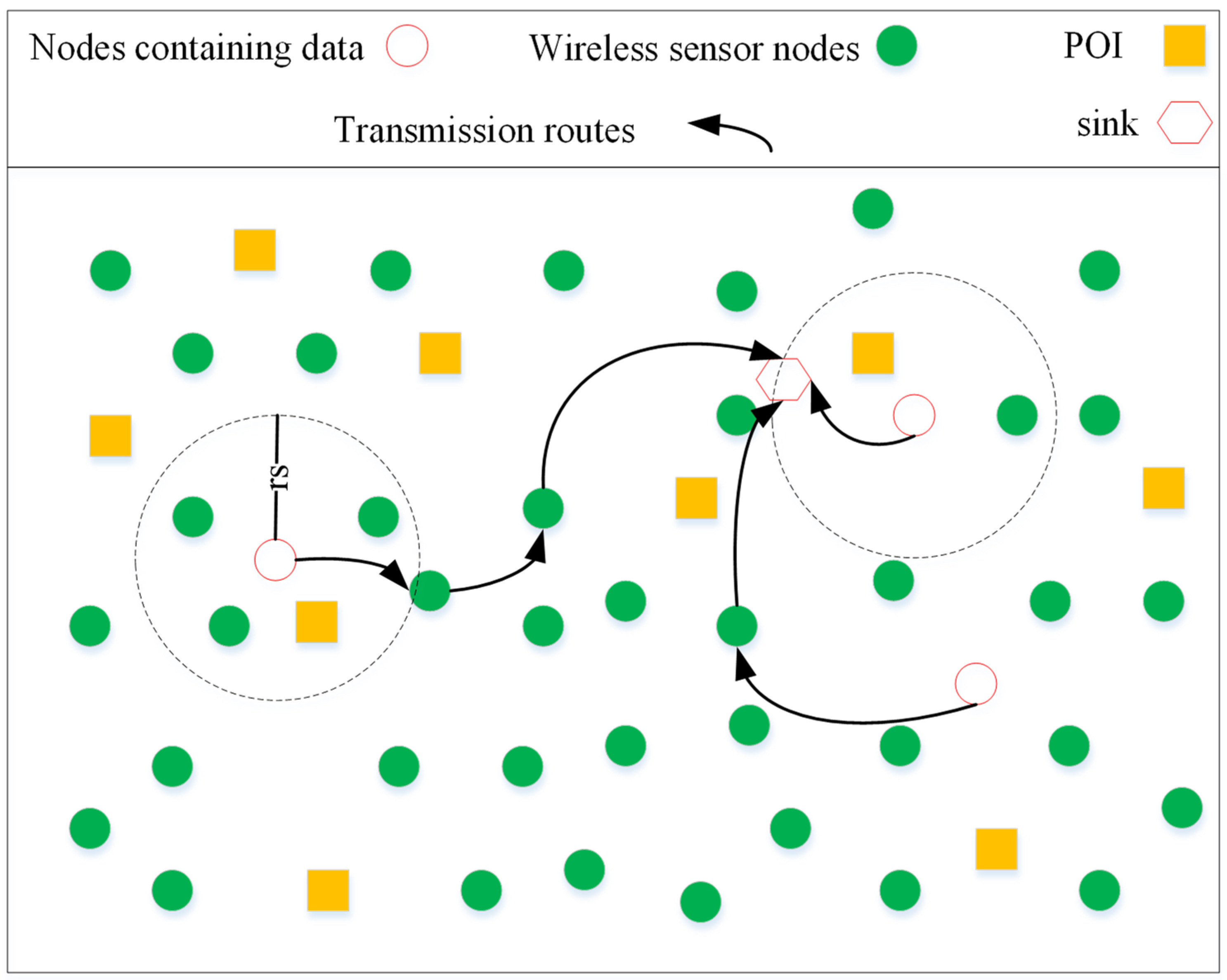
In this section, the method of using the suggested improved dragonfly optimization algorithm for solving the coverage problem in wireless sensor networks is performed. Each object is assumed to be equal to one sensor node in dragonfly relations, such that all of the sensor nodes and the sinks have a fixed location after being arranged. Nodes were homogeneous and with the same communication capacities of the range for sensing and capacities for data processing. The location of each sensor node is already recognized, and the well knows the location of all of the nodes.
The radio range of the sensors is assumed to be
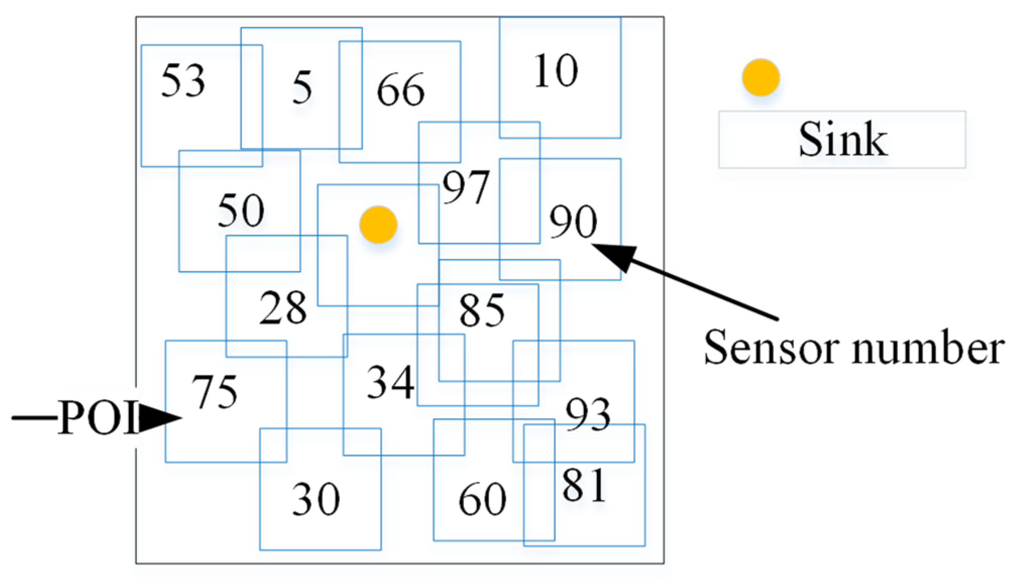
. The proposed algorithm assumes the problem of point coverage in a certain environment. As a result, outlier sensors (sensors that are not in the coverage area) will be removed. The point of interest (POI) is the place where the event takes place. It is assumed that the event signal can always be generated in all POIs.
Figure 1 shows sending events at star points by neighboring nodes to the sink.
As can be observed from
Figure 1, each POI is enclosed by some sensor nodes. If the POI is in the interior of the range of the radio radius,
, of a certain sensor, the sensor node detects the event signal and sends the restrained data to the well in multistep.
The target environment, is a two-dimensional surface, square meters.
Some sensor nodes in
have been described by
, where
and
define the sensor nodes’ quantity. The coordinates and radio beam of a sensor node are defined by
and
, respectively. Some POIs distributed in region
are determined by
, where
has been placed at
in
, and
is the number of POIs. The binary variable
in the following equation specifies whether
is able to cover
or not:
If the distance between
and
provides small value then the
, then
will be covered by
. Therefore, the event signal made in the POI can be identified. Although
can be simultaneously covered by
sensor nodes, if a specific
has been sheltered by more than one sensor node, then the union of
for
is calculated by the Boolean (binary) operator:
where,
is the Boolean inverse of
. The operators
and
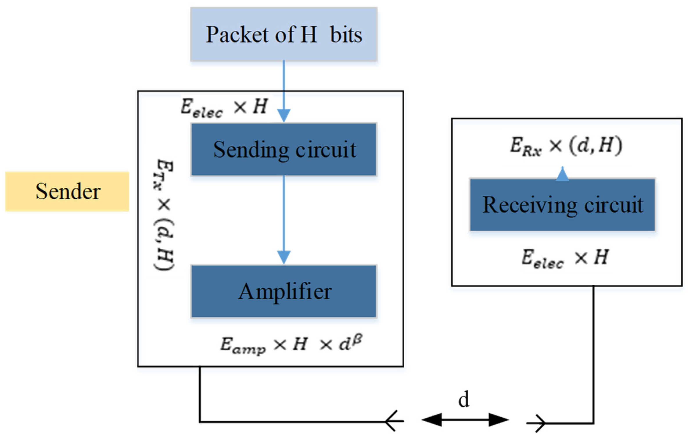
represent the symbol of the Boolean union and intersection. The energy consumption model is shown in
Figure 2. Therefore, most of the energy used in radio transmission is in the general operation of the sensor and access to the memory, so other energy-consuming matters are overlooked.
In the above Figure,
represents the energy lost in the transmission circuit or the receiving circuit per bit (in nanojoules).
indicates the energy consumed by the power amplifier per bit and
is the power of the path. The value of
is usually taken as 2. As a result, when an H-bit packet is sent to the receiver, the total energy consumed is calculated as follows:
where
and
represent, in turn, the overall energy used to send and receive an H-bit packet.
Since all of the sensor nodes are supposed to be homogeneous, their initial energy is the same. However, the energy of the sink is high and is not included in this energy consumption model. The set covering problem (SCP) is an NP-hard problem [
35].
In this article, this concept is implemented on the node scheduling optimization, which contains the issue of coverage management along with energy efficiency. In fact, the SCP is the problem of finding some nodes with minimal costs, where desired points are enclosed by no less than one node. Therefore, the set covering problem can be defined as follows:
Such that:
where,
is the activation cost of each node and
means activation and
means inactive (for outlier sensors). The constraint of the equation above states that every
is enclosed by no less than one node. After the network activates, it is necessary to use the optimization model described in the above relation, because this model optimizes energy consumption in the network. In the prosed improved dragonfly optimization algorithm, each dragonfly signifies a solution with a conforming cost value, which results in the cost function. The cost function (objective function) is utilized to find the quality of the solution. After applying the algorithm, a new population with better members is produced. Additionally, the process stops when it reaches the stopping condition.
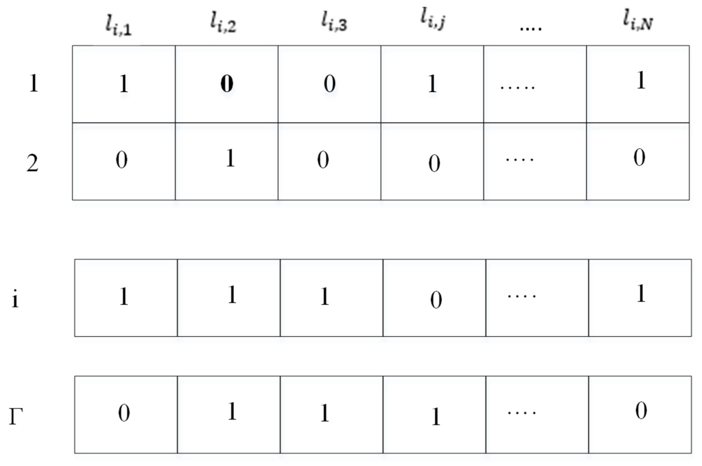
The better coding of individuals can increase the algorithm’s efficiency. To optimize the energy-aware coverage, it is necessary to code the scheduling of the nodes. This research employs optimal node scheduling to activate and deactivate wireless sensor nodes at a definite time in such a way as to raise the network’s lifetime. For programming, the solutions are displayed as binary strings. For instance, 0 indicates that the sensor node is inactive (eliminated), and 1 indicates that the node is active. The binary illustration of individuals in the improved dragonfly optimization algorithm for energy-aware coverage optimization is shown in
Figure 3.
In this figure,
represents the total quantity of members (candidates) and
signifies the state of the node
in individual
. It should be noted that the length of each individual is equal to
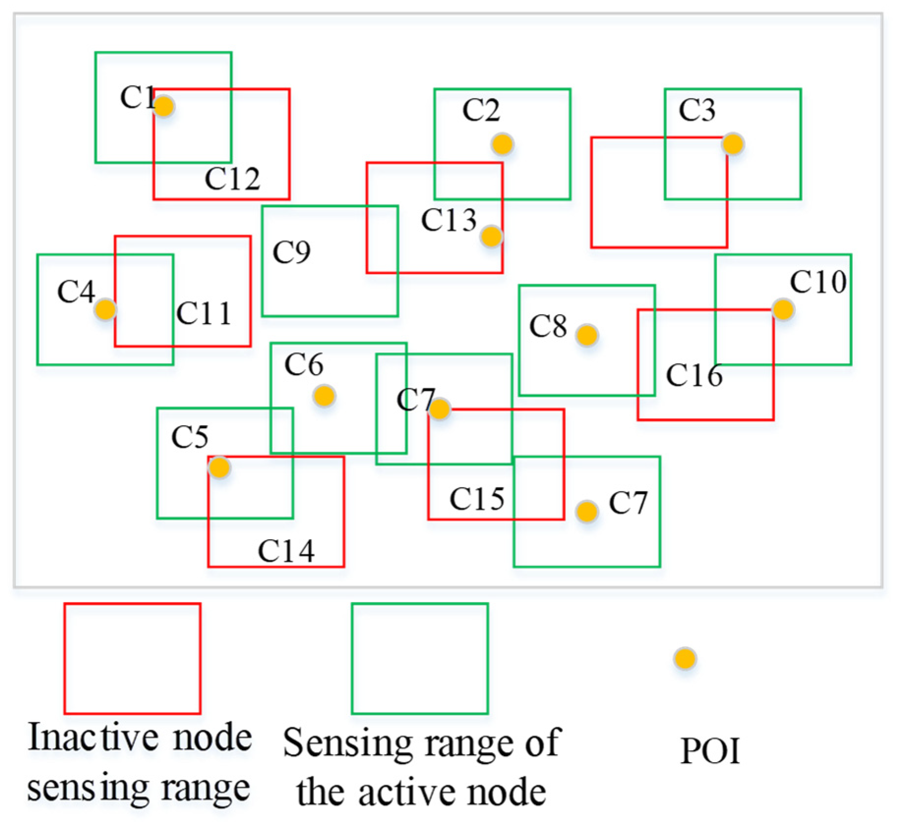
, which means the number of sensor nodes. Since the size of the population causes the production of diverse communities, it is necessary to choose an appropriate size of the population. For the sake of simplification, the population size is determined before running the algorithm; therefore, the size of the population is constant in each iteration of the algorithm. In
Figure 4, 16 nodes are used to sense the environment, and there are several additional nodes (15) (red circles).
To conserve energy and obtain the optimal coverage ratio, there is an optimal scheduling of nodes in the algorithm, which disables the redundant nodes. From the point of view of encoding particles, string 1111111111000000 represents the example in
Figure 4.
The fitness function has been utilized to measure the quality of the candidates. The purpose of the algorithm is to obtain the optimal coverage ratio using the least amount of sensor nodes. For nodes, a coverage vector has been suggested that represents the POIs’ coverage.
As stated by the coverage model defined previously, the coverage vector of a specific node
is demarcated by
. A binary model is used to know the coverage of a POI by a wireless sensor. Boolean operators are applied to vectors. A composite covering vector of
and
can be obtained by the Boolean union between
and
:
where,
is a combined coverage vector that shows the coverage or non-coverage of all POIs by
and
.
The combined coverage vector for a particular individual is calculated by the following equation:
The process of checking the coverage has been simplified to binary operators. The coverage ratio for every one,
, is:
where,
indicates the active nodes quantity. The nodes utility ratio,
, for individual
is evaluated as follows:
The nominator of the relation signifies the nodes quantity selected for activation. The quality of individual
is defined by
:
Substituting
and
from the above equations, we have:
where,
and
are the weighting constants, and
and
represent the power factors.
5. Simulation Results
In the implementation and evaluation, we used an Intel® Core ™ i5-4460 CPU @3.20 GHz processor, 12 gigabytes of memory, and a Windows 10 (64-bit) system. The efficiency of the proposed method was evaluated using MATLAB software. The algorithm of the proposed method was implemented in this software, and simulations were carried out at different stages. MATLAB optimization functions were used in the process. The simulation work was repeated up to 2500 steps until the results reach a stable point.
In this study, we compared the proposed method with three methods from the literature, including the LEACH [
35], RED-LEACH [
36], and gravitational search algorithm (GSA)-based methods [
37]. The LEACH method is one of the first clustering methods in sensor networks. In the proposed method, four parameters are used to evaluate the efficiency:
- ○
The quantity of nodes in the exposure zone: The coverage area includes the area where the nodes are located.
- ○
Network lifetime: The network lifetime includes the time from the beginning of the first node to the time when the first node dies.
- ○
Network capacity: The ratio of the number of packets received by the well to the quantity of packets sent by the nodes.
- ○
Residual energy: The remaining energy in the battery of the sensor nodes is used to analyze the energy consumption in each method.
In this scenario (
Figure 5), the sink is placed in the center of a WSN.
Nodes are clustered, and each cluster head sends data directly to the sink without the use of an auxiliary node. The objectification parameters of this scenario are explained in the following information: The size of the grid in this study is set to 100 × 100 . The main station location is (60, 120). The sensor node quantity is 110. The size of the data package is set at 500 bytes, is set 50, the is set 10, the value of the is considered 0.0010, and the initial energy is set at 0.5 joules.
5.1. The Number of Nodes in the Coverage Area
The sensor nodes are usually randomly distributed in a network, and the area covered by them is shown with a circle. In
Figure 5, the proposed improved dragonfly optimization algorithm is applied to this network. As seen in
Figure 5, the coverage area and the number of active nodes has been optimized. Decreasing the number of active sensor nodes leads to a decrease in energy consumption and, as a result, to an increase in the lifetime of the network.
5.2. Network Lifetime
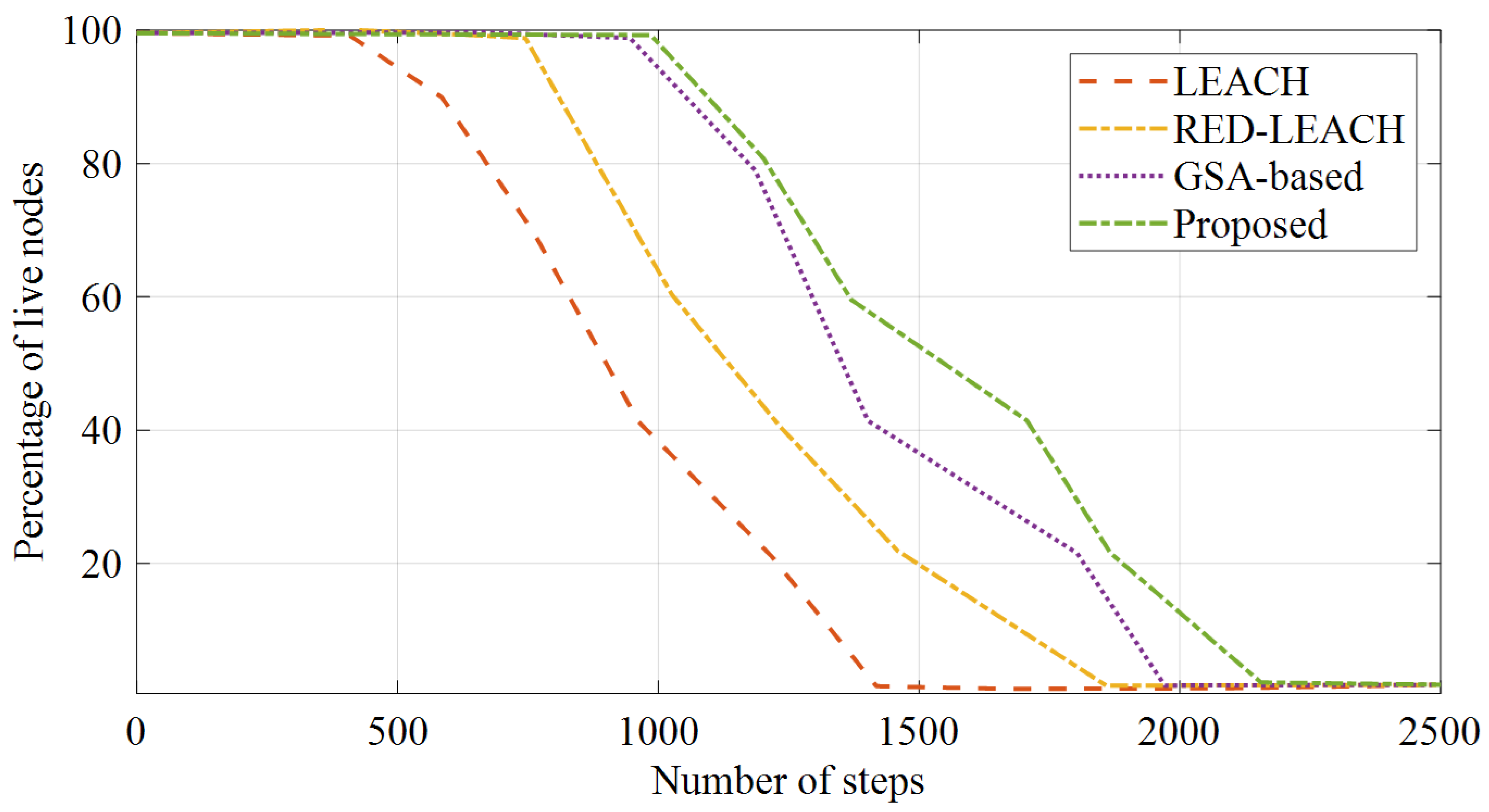
The number of live nodes is shown in
Figure 6. These numbers are for the proposed method, the LEACH method [
23], the RED-LEACH method [
27], and the gravitational search algorithm (GSA)-based method [
37]. In this diagram, the initial energy of the sensor nodes is assumed to be half a joule.
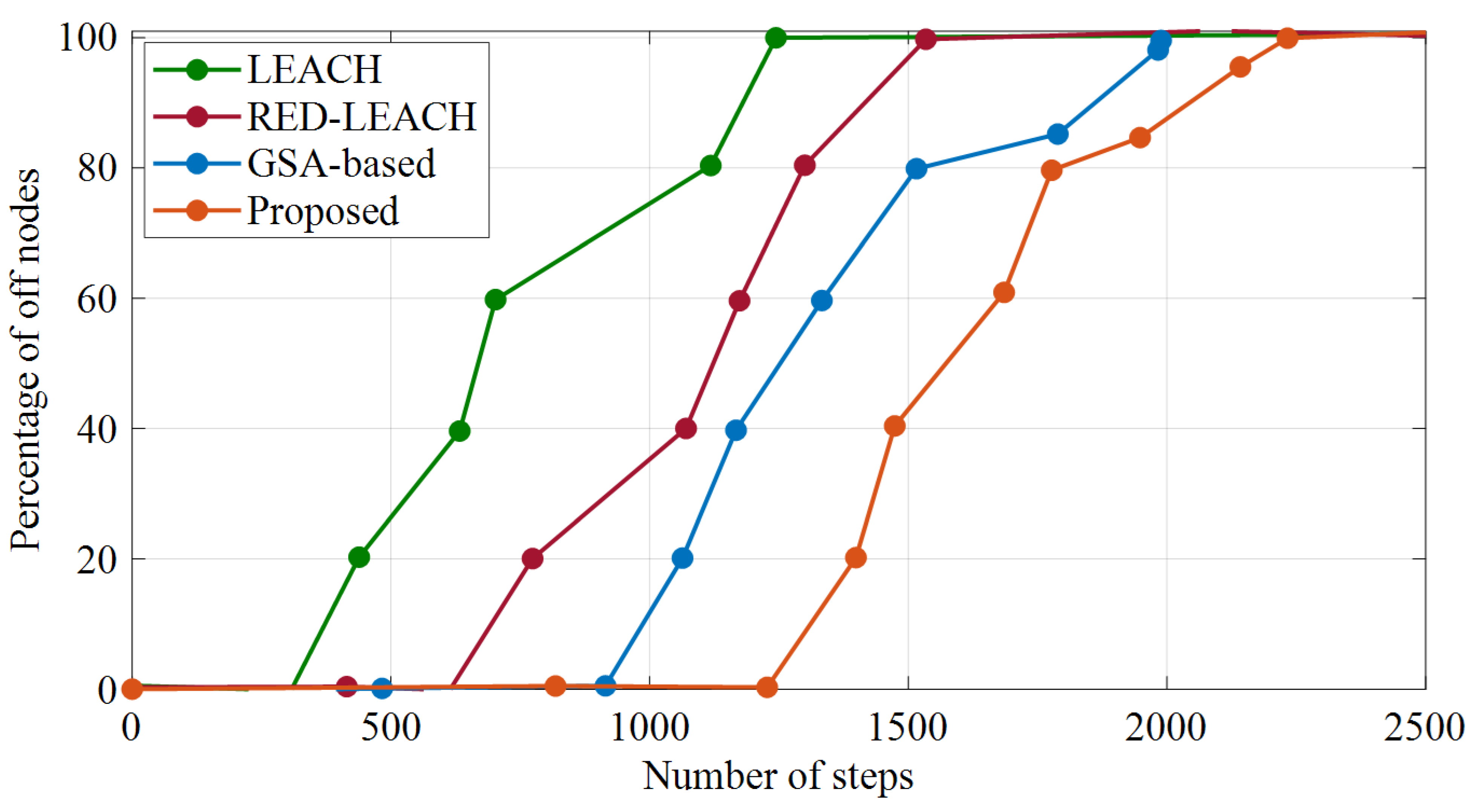
Figure 6 shows the network lifetime based on the analyzed methods, and
Figure 7 shows the number of off nodes.
It can be perceived from
Figure 7 that, by increasing the number of steps, the energy of the live nodes will eventually run out and turn off. In the LEACH method, after 350 steps, the RED-LEACH method, after 750 steps, and the GSA-based method, after 915 steps, the nodes start shutting down, which occurs after 1227 steps for the proposed method. This means that the nodes are turned off later. Since the first node’s shutdown time is considered in defining the lifetime of the network, this figure indicates that the suggested method offers a longer lifetime. The reason for this improvement is that the proposed method distributes the consumed energy in a balanced way among the network nodes. On the other hand, by increasing the number of steps, the percentage of live nodes in the proposed method works better than that of the other methods. This method means that after almost 2155 steps all of its nodes are turned off, and, until then, the probability of establishing a route for sending packets is higher than that of the other methods.
As can be seen in
Figure 6, all of the network nodes in the LEACH method lost their energy after approximately 1418 steps, after 1859 steps for the RED-LEACH method, and after 1971 steps for the GSA-based method, while in the proposed method this event occurs after 2155 steps. This makes the nodes active in the network for a longer period of time and raises the network’s lifespan.
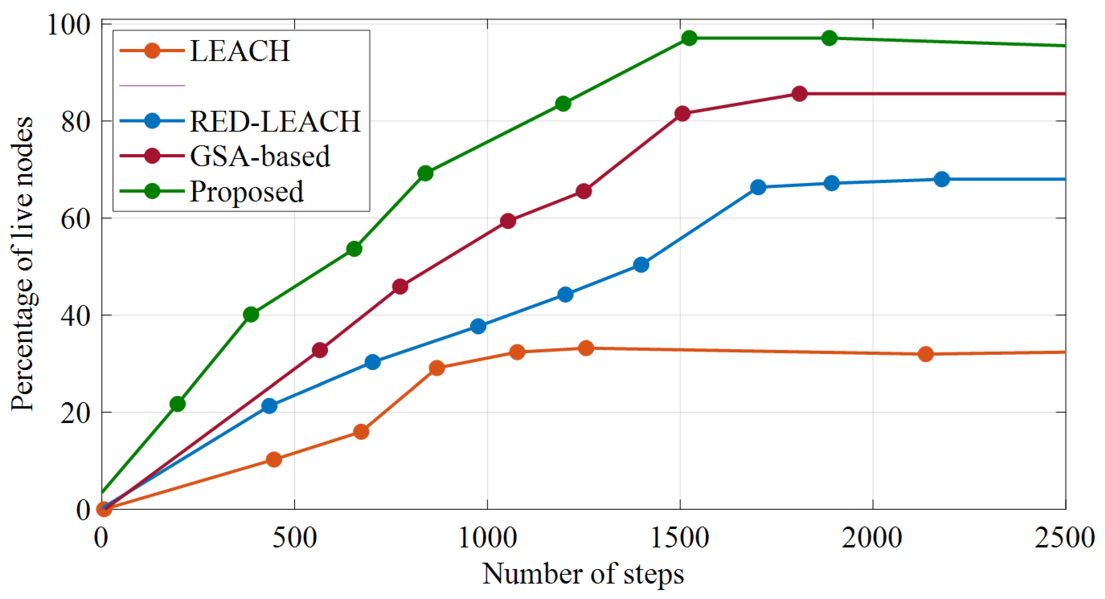
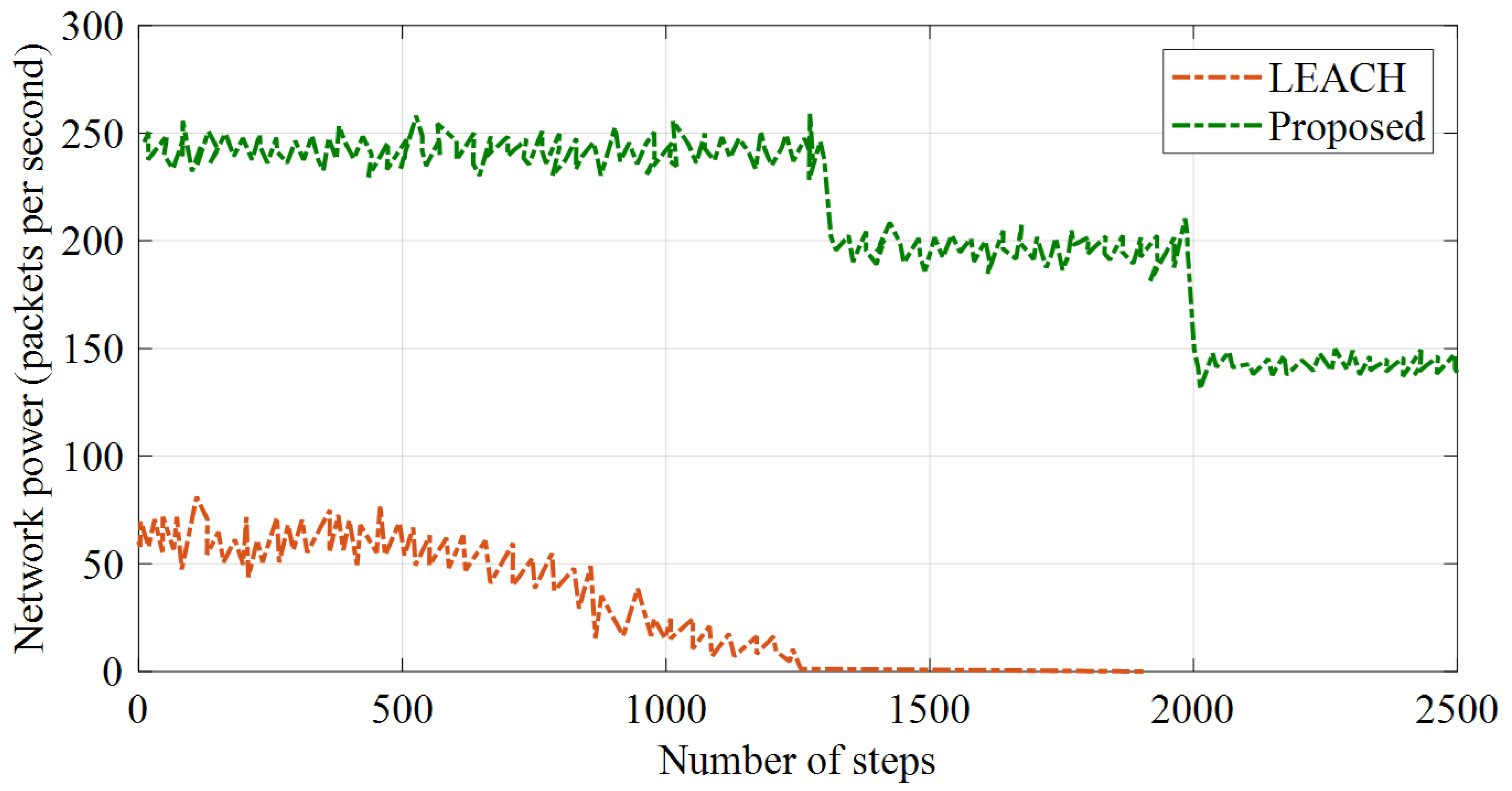
5.3. Throughput (Network Power)
The throughput can be calculated based on two criteria, including the average received packets in the network and the average sent packets to the sink. The averages of the sent and received packets to the sink node were obtained during repeated simulations for the assessed methods. The simulation outcomes showed that the proposed method increased the power of the network. These results are shown in
Figure 8 and
Figure 9.
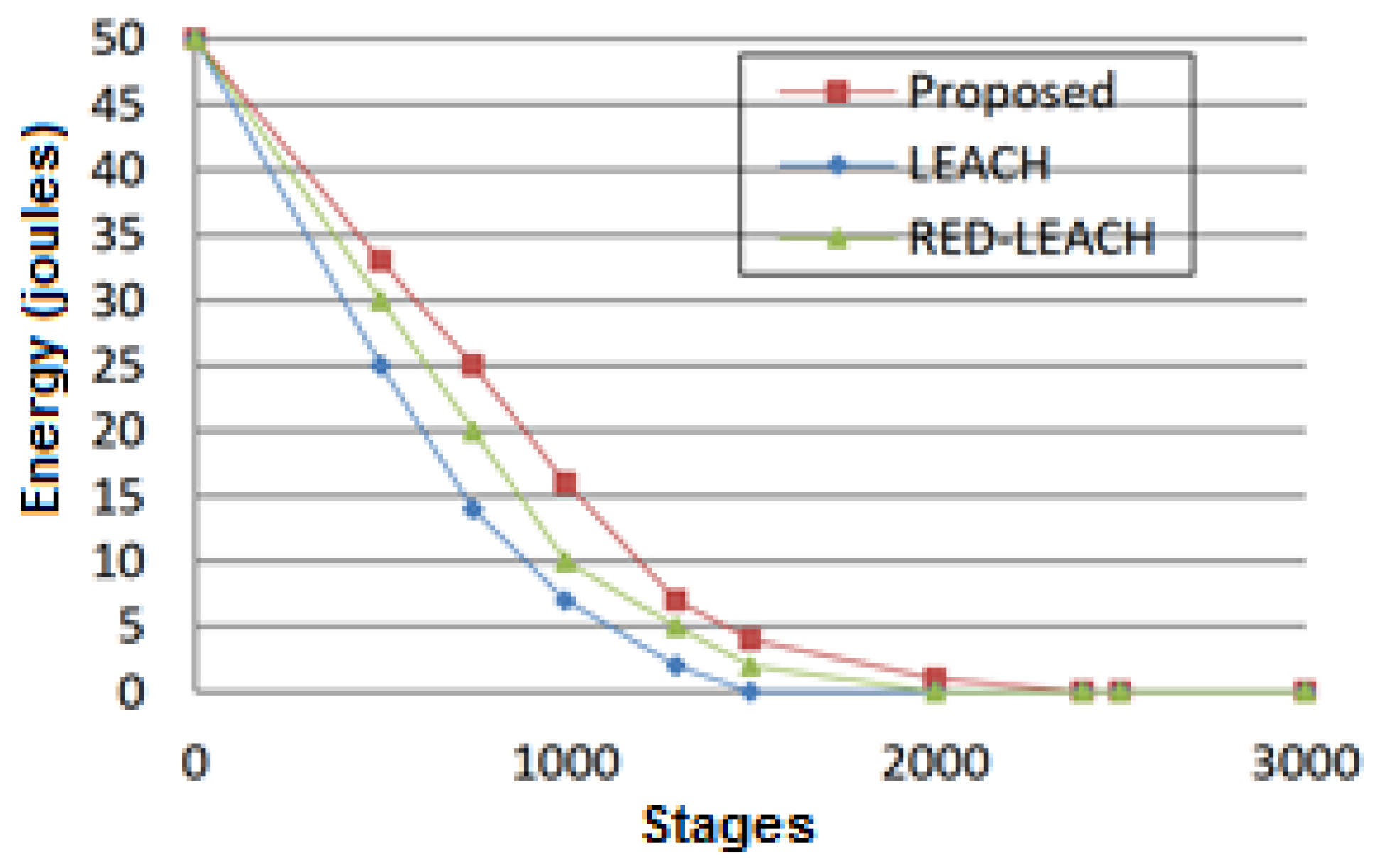
5.4. Residual Energy
Figure 10 shows the average residual energy in each stage. Here, it is assumed that each node has an initial energy of half a joule. In this case, the network total energy with 110 sensor nodes is equal to 50 joules.
It can be concluded from
Figure 10 that the remaining energy in the network decreases with an increase in the number of steps. The slope of this reduction is lower in the proposed technique. Accordingly, this method will have a longer network life. Additionally, the total energy of the network in the LEACH method reaches zero after 1500 steps, after 2000 steps in the RED_LEACH method, after 2400 steps in the PID_LEACH method, and after 2000 steps in the GSA-based method. This means that the probability of sending packets in the suggested technique will be higher than that of the other assessed methods with an increase in the number of data transfer rates.
As is observed, the proposed method has several advantages for the detection of IoT outlier sensors; however, it has also some shortcomings. Some of these shortcomings have been explained previously:
- ○
The issue is that there is not a specific way to solve it.
- ○
There is a precise solution to the issue and carrying it out incurs computational costs.
- ○
There is no determinate metaheuristic method that can solve any kind of similar problems.
6. Conclusions
The Internet of things is rarely discussed without a conversation about new ecosystem data and information. The intelligence and value of an Internet of things (IoT) system are using what may be learned from data, and sensors are the main sources of these data. The subject of collecting and sending information by objects specifically refers to sensors. Sensors can be used for sensing temperature, proximity, pressure, movement, position, humidity, light, air quality, or anything else. These sensors, coupled with Internet connectivity, enable them to automatically collect data from the environment, enabling stakeholders to make smarter decisions. Sensor networks are used in various fields, and there are primarily problems with sensor costs and battery replacements. Therefore, using the minimum number of sensors with full coverage and elimination is an incredibly important subject. In this paper, a new approach was attempted to detect outlier data and eliminate them in the Internet of things. Outlier sensors are one of the challenges of this type of network. In this paper, an improved version of the dragonfly optimization algorithm was used for optimal area coverage and energy consumption reduction. This paper used four parameters to evaluate its efficiency: the minimum quantity of nodes in the coverage area, the lifetime of the network, including the time interval from the start of the first node to the shutdown time of the first node, and the network power. The results of the suggested approach were compared with some published techniques. Simulations showed that the suggested technique achieved better results than the other investigated methods in terms of the provided performance parameters. The goal of future research is to construct IoT sensors that are appropriate for outlier detection modules (ODMs), analyze the sensors’ produced spatial–temporal data in real time, and create a testable IoT prototype with an integrated ODM. The investigation of potential computational constraints for the ODM will also be a key component of the project. Additionally, the effectiveness of the IoT will be examined, as will its capacity to correctly identify any malfunctioning sensors as well as the type, source, and impact of errors on these sensors.


