
An Enhanced ELECTRE II Method for Multi-Attribute Ontology Ranking with Z-Numbers and Probabilistic Linguistic Term Set


Abstract
:1. Introduction
- 1.
- The existing MCDM solutions for ranking ontologies [14,15,16,17] to aid their selection focus on ranking ontologies from a singular perspective. However, in real-world application, the ranking and selection of suitable ontologies for reuse would involve more than a single person. Rather, a group of experts and stakeholders would collectively evaluate and decide on the suitable ontologies to reuse. At present, very little emphasis has been placed on ontology ranking and selection in a group setting in the existing literature.
- 2.
- In real-world scenarios, ontologies would be ranked and selected not just according to their underlying characteristics, but a lot of importance would be given to how well the ontologies align with the needs and requirements of the organization and its stakeholders. However, the current MCDM solutions for ranking ontologies to aid their selection [14,15,16,17] focus on ranking ontologies based on their underlying characteristics and attributes. Little work has been completed that performs ontology ranking with MCDM methods from the perspectives of the actual users and knowledge engineers.
- 3.
- The current MCDM solutions for ranking ontologies [14,15,16,17] to aid their selection rely on quantitative metrics represented with numerical values to evaluate and rank the ontologies; this renders the task of decision-makers and subject experts very difficult, as they are required to handle a large number of numerical values to express their evaluation of alternatives in the process of ranking ontologies. It would be valuable to allow decision-makers and subject experts to use natural language and linguistic terminologies to express their views in the ranking process of ontologies. At present, very little work has been completed pertaining to the usage of linguistic modeling in MCDM solutions for ranking and selection of ontologies.
2. Literature Review
3. Preliminaries
3.1. ELECTRE II
3.2. Linguistic Term Set and Hesitant Fuzzy Linguistic Term Set
3.3. Probabilistic Linguistic Term Set
3.4. Z-Number
3.5. Z-Probabilistic Linguistic Term Set
- 1.
- is increased by adding ϕ terms to , where . The ϕ linguistic terms to be added may be any linguistic terms in .
- 2.
- The probabilities of the ϕ linguistic terms that were added must be set to 0.
- 1.
- If then .
- 2.
- If then .
- 3.
- If then the deviation degree is required to compare and as follows:
- (a)
- If then .
- (b)
- If then .
- (c)
- If then .
- (d)
- If and then .
4. ZPLTS-ELECTRE II
4.1. Quantitative Matrix
4.2. Decision-Makers Evaluation Matrix
4.3. Decision Matrix
4.4. Weights and Thresholds
4.5. Comparative Sets
4.6. Concordance Relations
4.7. Discordance Relations
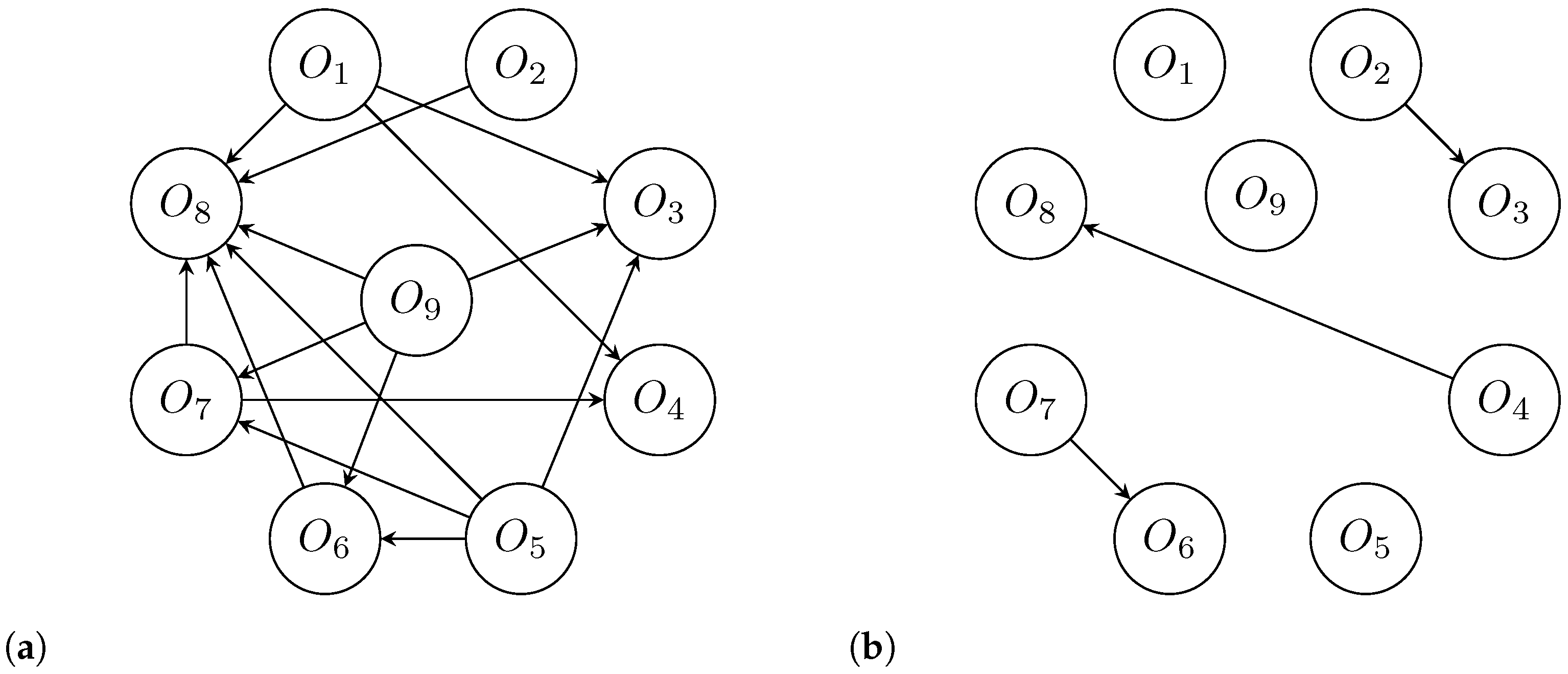
4.8. Strong and Weak Outranking Graphs
4.9. Exploit Outranking Relations
- 1.
- Let denote the set of non-dominant alternatives in the strong outranking graph . is filled by all those alternatives that are not outranked by any other alternatives, that is, all those alternatives that have no arcs going into them. The same is completed for the weak outranking graph, , with the set .
- 2.
- The intersection of and , , is determined to produce the set . The alternatives in are those that are not outranked in both the strong and the weak outranking graphs. All those alternatives in are given the forward rank of 1, that is, for all alternatives in .
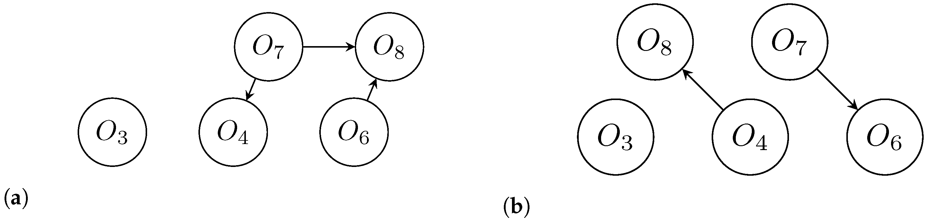
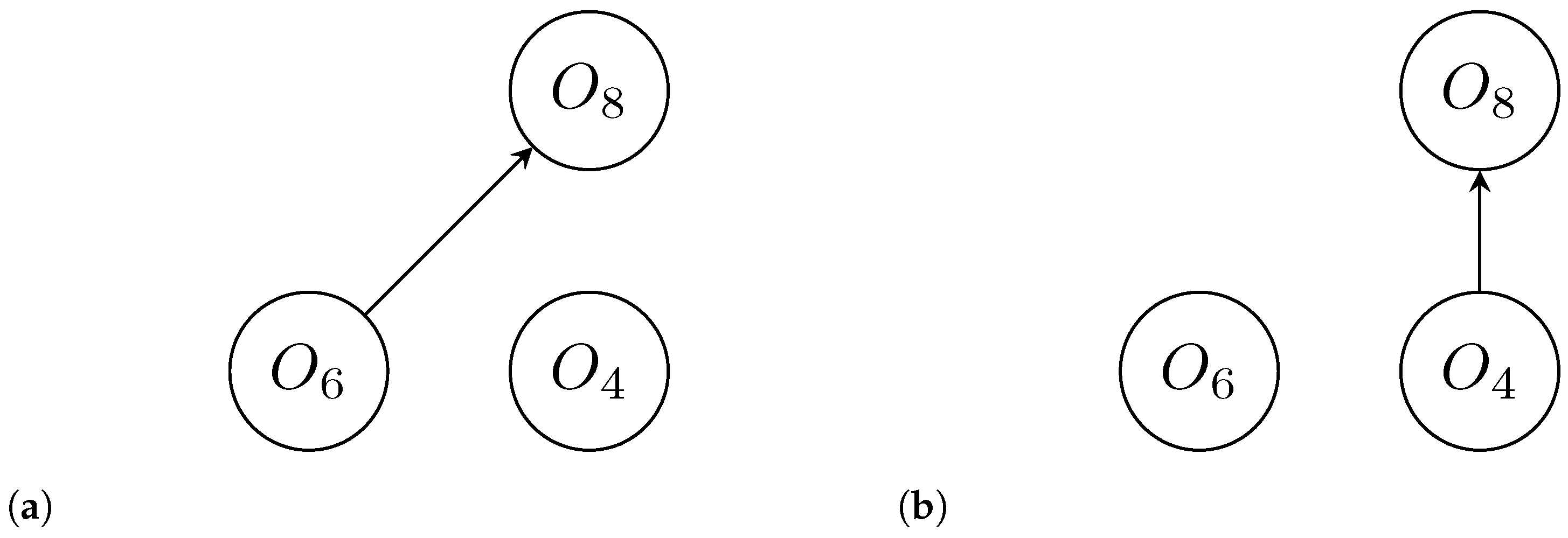
- 3.
- The nodes of those alternatives contained in can now be removed from the strong outranking and the weak outranking graphs along with their associated edges. After removing the nodes and edges, the resulting graphs are and .
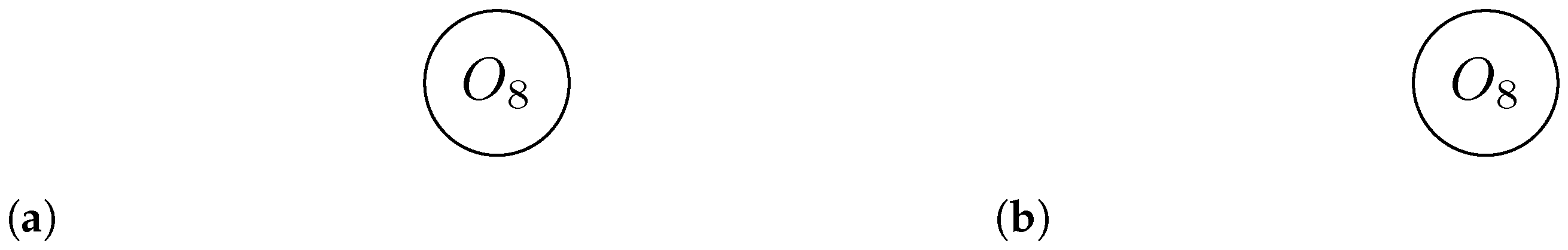
- 4.
- The steps 1 to 3 are repeated until all alternatives have been ranked, with each iteration producing a new set of graphs and . Eventually, all alternatives should be assigned a forward rank.
- 1.
- All the arrows in the strong and weak outranking graphs, and , are reversed to form the mirror image graphs.
- 2.
- Each alternative is assigned a rank, , in the same way as in the forward order from steps 1 to 3.
- 3.
- Due to the graph reversals, each rank is transformed by applying Equation (28).
| Algorithm 1 ZPLTS-ELECTRE II. |
|
5. Application of ZPLTS-ELECTRE II Method in Ontology Ranking
5.1. Experimental Design
5.1.1. Dataset
- 1.
- The Mental State Assessment Ontology (ONL-MSA)—ONL-MSA is a module of the OntoNeuroLOG [56] ontology, which was developed in the NeuroLog (http://neurolog.i3s.unice.fr/ accessed on 21 August 2022) project for enhancing the field of neuroimaging. The ONL-MSA ontology models knowledge pertaining to the mental state assessments.
- 2.
- The APA Neuro Cluster Ontology (APANEUROCLUSTER)—it models the APA neuropsychology and neurology and includes the Assessment Diagnosis, Neurosciences, Neurological Disorders, and Neuroanatomy categories.
- 3.
- The Ontologia de Saúde Mental (OSM)—it is the Portuguese equivalent of Mental Health Ontology, it was developed to assist in managing the Psychosocial Care Network in the Brazilian context, enabling the creation of intelligent computational tools and the development of mental health indicators.
- 4.
- The Mental Functioning Ontology (MF)—it is an ontology that represents aspects of mental functioning, such as cognition and intelligence.
- 5.
- The Alzheimer’s Disease Ontology (ADO)—it represents knowledge regarding Alzheimer’s disease. The main categories of the ontology include Health, Human, Neurologic Disease, and Neurological Disorder.
- 6.
- The Neuroscience Information Framework Cell Ontology (NIFCELL)—it is part of the Neuroscience Information Framework (NIF) project (http://neuinfo.org accessed on 21 August 2022). The NIFCELL ontology expresses knowledge regarding cells and cell types from the Neuroscience Information Framework Standard Ontology (https://bioportal.bioontology.org/ontologies/NIFSTD accessed on 21 August 2022).
- 7.
- The Epilepsy Semiology Ontology (EPISEM)—it was designed to capture the semiology of epilepsy. It models the signs and symptoms of epilepsy and represents the ictal, post-ictal, inter-ictal, and aura signs.
- 8.
- The Cognitive Paradigm Ontology (COGPO) (http://www.cogpo.org/ accessed on 21 August 2022)—COGPO was developed to describe the experimental conditions within experiments related to the cognition and behavior of humans. The ontology defines the conditions of experiments in a standardized format.
- 9.
- The Cognitive Atlas Ontology (COGAT) (https://www.cognitiveatlas.org/ accessed on 21 August 2022)—COGAT models and characterizes the state of current thought in cognitive science through a set of mental concepts and tasks. The ontology represents users’ knowledge with expertise in psychology, cognitive science, and neuroscience.
5.1.2. Quantitative Attributes
- 1.
- The Absolute Leaf Cardinality metric, abbreviated ALC, is an indicator of the number of leaf nodes within a graph [58,59]; it expresses the dispersion of leaf nodes within a graph and is calculated by Equation (30).where m is the ALC metric, and n is the cardinality of the set , which is a subset of the directed graph g.
- 2.
- 3.
- Depth is a graph property of an ontology relating to the number of paths within the graph, considering the taxonomy is-a arcs only. The Average Depth metric, abbreviated AD, is determined by dividing the sum of the cardinalities of every path within a graph, by the cardinality of the set of all paths in that graph [58]. The AD is an indicator of the degree to which an ontology has a vertical modeling with many taxonomy is-a relations, which represent richer information content in the ontology [60]. The AD metric is calculated by Equation (32).where m represents the AD value, N is the cardinality of the paths j, P represents the set of paths within the graph g, and n represents the cardinality of P.
- 4.
- The Average Breadth metric, abbreviated AB, expresses the average cardinality value of a generation in a graph. It is calculated by dividing the sum of the cardinalities of all generations by the number of generations in the graph [58]. The metric is an indicator of the degree to which the ontology has a horizontal modeling of its hierarchies with less taxonomy is-a relations [60]. The AB metric is calculated by Equation (33).where m represents the AB value, N is the cardinality of a generation, j a particular generation, is the cardinality of L, and L is the set of all generations within a graph g.
- 5.
- The Average Number of Paths, abbreviated ANP, expresses the relationship between a concept and the root concept within the taxonomy hierarchy of the ontology. An ontology that has a high ANP value contains a large number of taxonomy/inheritance relationships along with a large number of interconnections between the classes within the ontology. If the ANP value is 1, then it signifies that the inheritance hierarchy of the ontology is a tree [61]. The ANP is calculated by Equation (34).where m is the ANP value, is the number of paths for a given concept, and is the total number of concepts.
5.1.3. Qualitative Attributes
- 1.
- Clarity of Purpose (CoP)—This criterion addresses the question of how clear is the purpose of the ontology [27]. The CoP criterion pertains to the semantics and documentation of the ontology.
- 2.
- Quality of Subclass Definition (QoSD)—This criterion addresses the question of how properly the subclasses in the ontology are defined and whether the class hierarchy needs better organization or not [27]. The QoSD criterion pertains to the syntax and structure of the content of the ontology.
- 3.
- Description of Concepts and Relations in Natural Language (DoCRNL)—This criterion describes how well the concepts and the relations of an ontology are described using natural language [27]. The DoCRNL criterion is expressive of the semantics and documentation of the ontology.
- 4.
- Understandability of Conceptualization (UoC)—This criterion expresses how easy it is to comprehend the ontology’s conceptualization [27]. The UoC criterion pertains to the semantics and documentation aspects of an ontology.
- 5.
- Description of Concepts using Attributes (DoCA)—This criterion concerns how well the attributes in the ontology describe its concepts [27]. The DoCA criterion pertains to the information content of the ontology.
5.1.4. Computer and Software Environments
5.2. Experimental Results and Discussions
5.2.1. Quantitative Matrix
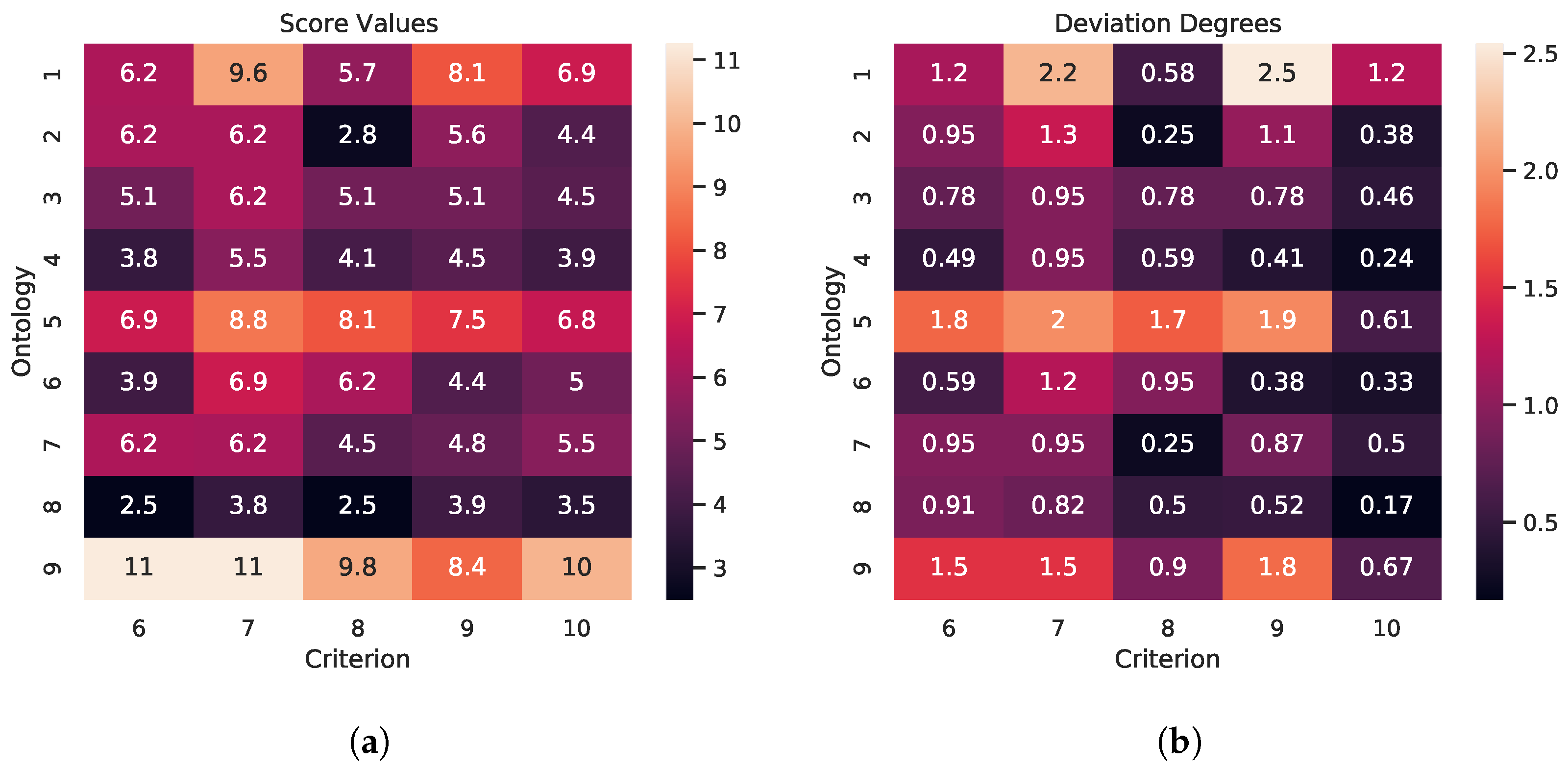
5.2.2. Qualitative Matrices
5.2.3. Decision Matrix
5.2.4. Weights and Thresholds
5.2.5. Comparative Sets
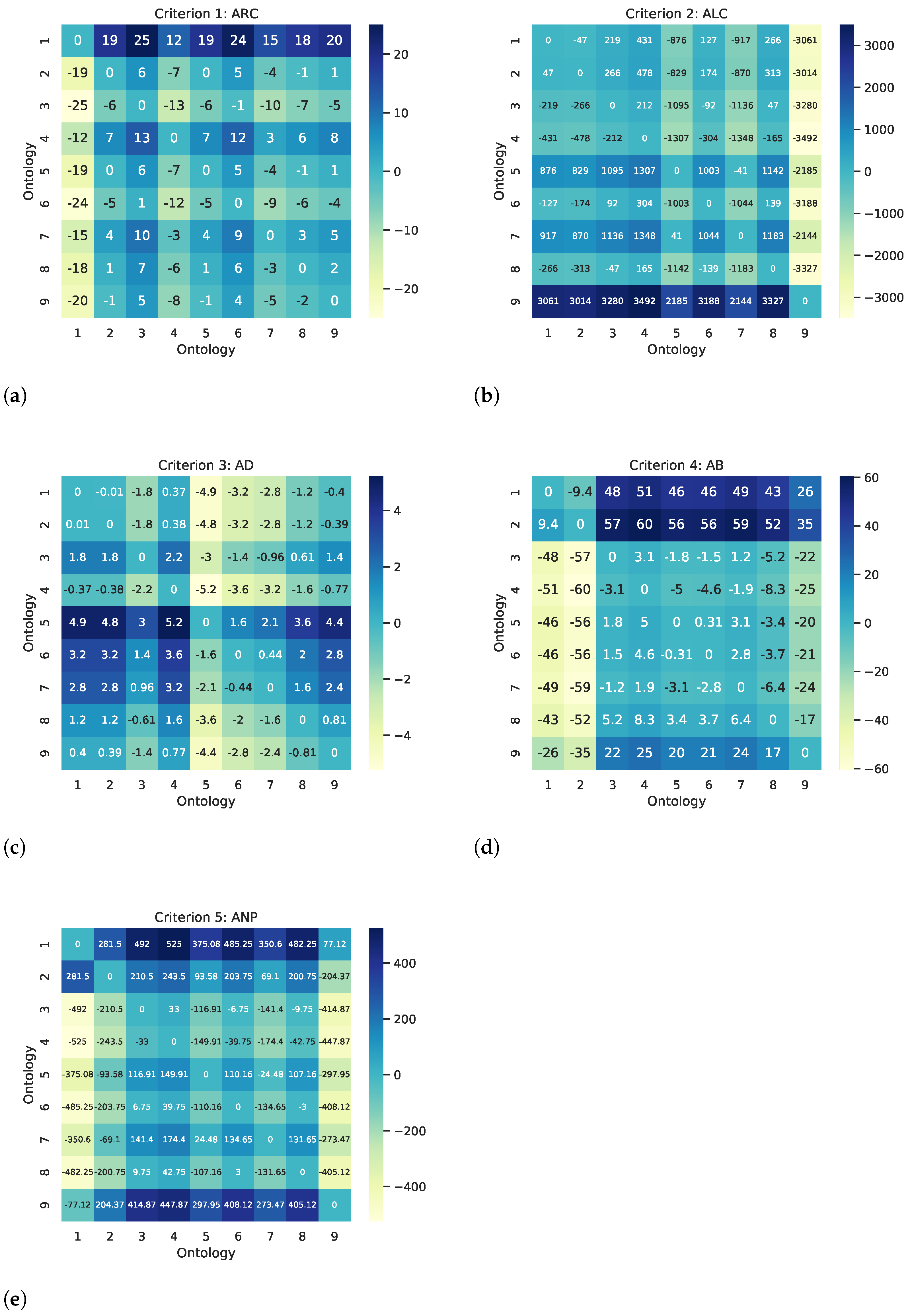
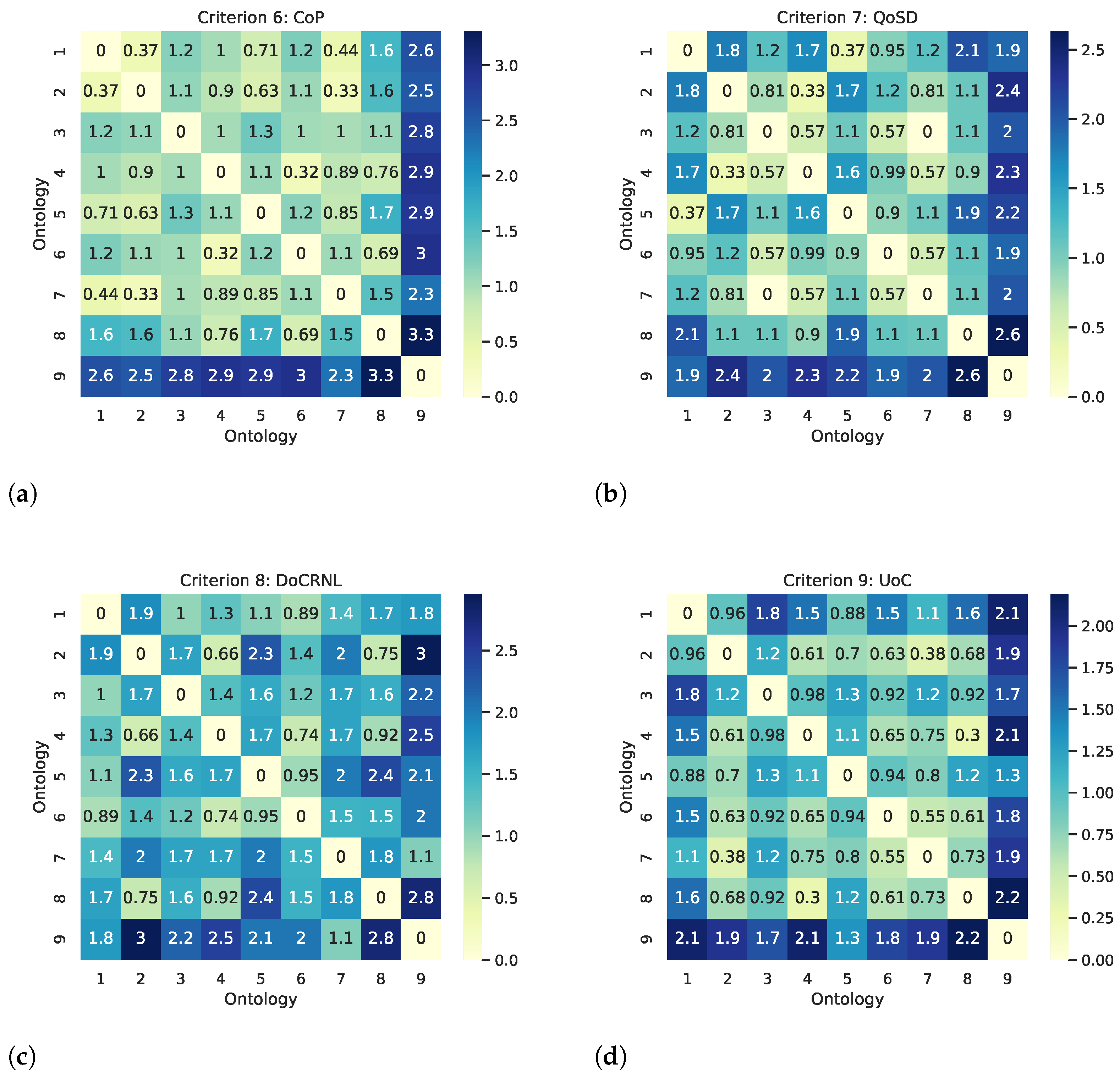
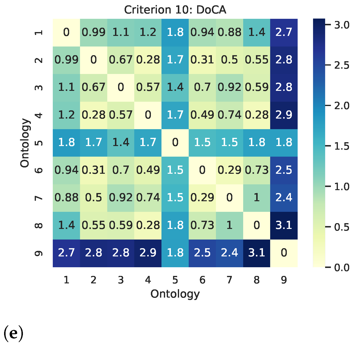
5.2.6. Concordance Relations
5.2.7. Discordance Relations
5.2.8. Strong and Weak Outranking Graphs
5.2.9. Exploitation of Outranking Relations
5.3. Comparative Analysis of ZPLTS-ELECTRE II
5.3.1. Comparison with Traditional ELECTRE II
5.3.2. Comparison with PLTS ELECTRE II
5.4. Discussion
5.4.1. Comparison with Existing MCDM Methods for Ontology Ranking
5.4.2. Comparison with Existing Fuzzy ELECTRE II Methods
5.4.3. Strengths of ZPLTS-ELECTRE II
- 1.
- The method can model both quantitative numerical and qualitative linguistic criteria, thereby providing decision-makers with more flexible and realistic expression of their preferences.
- 2.
- Individual discordance thresholds can be specified for each criterion. This provides the decision-makers with more flexibility in expressing their preferences.
- 3.
- Decision-makers are able to express their level of confidence or credibility when providing their evaluations, thereby improving the ability of the model to capture the cognitive nature of the decision-making process.
- 4.
- The applications of the ZPLTS-ELECTRE II method are not constrained to ontology ranking, but rather, it can be applied to any decision-making problem in any domain.
5.4.4. Weaknesses and Limitations of ZPLTS-ELECTRE II
- 1.
- The different decision-makers are assigned equal weighting, and the final decision matrix is composed by combining the individual decision-makers’ evaluation matrices with equal importance given to all decision-makers. This may not be the case in some decision-making problems.
- 2.
- The ZPLTS-ELECTRE II method is dependent on the decision-makers for the specifications of the thresholds and parameters, such as the criteria importance weights, the concordance thresholds, and the discordance thresholds.
- 3.
- The ability of the ZPLTS-ELECTRE II method to model both linguistic and numerical data has the implication of individual discordance thresholds for each criterion. This is an advantage as it expands the method’s capability of modeling decision-problems. However, when comparing the method to other ELECTRE II methods, ZPLTS-ELECTRE II has the disadvantage of having a larger number of discordance thresholds to be analyzed and defined as opposed to other methods that may only require a smaller number of discordance thresholds.
6. Conclusions and Future Work
Author Contributions
Funding
Data Availability Statement
Acknowledgments
Conflicts of Interest
References
- Tang, X.; Li, X.; Ding, Y.; Song, M.; Bu, Y. The Pace of Artificial Intelligence Innovations: Speed, Talent, and Trial-and-Error. J. Inf. 2020, 14, 101094. [Google Scholar] [CrossRef]
- Gruber, T. A translation approach to portable ontology specifications. Knowl. Acquis. 1993, 5, 199–220. [Google Scholar] [CrossRef]
- Bhuyan, B.; Tomar, R.; Gupta, M.; Ramdane-Cherif, A. An Ontological Knowledge Representation for Smart Agriculture. In Proceedings of the 2021 IEEE International Conference on Big Data (Big Data), Orlando, FL, USA, 15–18 December 2021. [Google Scholar]
- Roman, D.; Alexiev, V.; Paniagua, J.; Elvesætera, B.; Zernichow, B.M.; Soylu, A.; Simeonov, B.; Taggart, C. The euBusinessGraph ontology: A lightweight ontology for harmonizing basic company information. Semant. Web 2021, 13, 1–28. [Google Scholar] [CrossRef]
- Stancin, K.; Poscic, P.; Jaksic, D. Ontologies in education—State of the art. Educ. Inf. Technol. 2020, 25, 5301–5320. [Google Scholar] [CrossRef]
- Chen, J.; Chen, Y.; Hu, Z.; Lu, J.; Zheng, X.; Zhang, H.; Kiritsis, D. A Semantic Ontology-Based Approach to Support Model-Based Systems Engineering Design for an Aircraft Prognostic Health Management System. Front. Manuf. Technol. 2022, 2, 1–21. [Google Scholar] [CrossRef]
- BioPortal Ontology Repository. Available online: https://bioportal.bioontology.org/ (accessed on 8 June 2022).
- AgroPortal Ontology Repository. Available online: http://agroportal.lirmm.fr/ (accessed on 8 June 2022).
- Alani, H.; Brewster, C. Ontology Ranking based on the Analysis of Concept Structures. In Proceedings of the Third International Conference on Knowledge Capture (K-Cap), Banff, AB, Canada, 2–5 October 2005. [Google Scholar]
- Alani, H.; Brewster, C.; Shadbolt, N. Ranking Ontologies with AKTiveRank. In Proceedings of the 5th International Conference on the Semantic Web, Athens, Greece, 1–15 November 2006. [Google Scholar]
- Yu, W.; Chen, J.; Cao, J. A Novel Approach for Ranking Ontologies on the Semantic Web. In Proceedings of the 1st International Symposium on Pervasive Computing and Applications, Xinjiang, China, 3 August 2006; pp. 608–612. [Google Scholar]
- Alipanah, N.; Srivastava, P.; Parveen, P.; Thuraisingham, B. Ranking Ontologies Using Verified Entities to Facilitate Federated Queries. In Proceedings of the 2010 IEEE/WIC/ACM International Conference on Web Intelligence & Intelligent Agent Technology, Washington, DC, USA, 31 August–3 September 2010. [Google Scholar]
- Subhashini, R.; Akilandeswari, J. A Novel Approach For Ranking Ontologies Based On The Structure And Semantics. J. Theor. Appl. Inf. Technol. 2014, 65, 147–153. [Google Scholar]
- Esposito, A.; Tarricone, L.; Zappatore, M. Applying multi-criteria approaches to ontology ranking: A comparison with AKTiveRank. Int. J. Metadata Semant. Ontol. 2012, 7, 197. [Google Scholar] [CrossRef]
- Fonou-Dombeu, J.V. Ranking Semantic Web Ontologies with ELECTRE. In Proceedings of the 2019 International Conference on Advances in Big Data, Computing and Data Communication Systems (icABCD), Winterton, South Africa, 5–6 August 2019. [Google Scholar]
- Fonou-Dombeu, J.V.; Viriri, S. CRank: A Novel Framework for Ranking Semantic Web Ontologies. Model Data Eng. (MEDI) 2018, 11163, 107–121. [Google Scholar]
- Fonou-Dombeu, J.V. A Comparative Application of Multi-criteria Decision Making in Ontology Ranking. Bus. Inf. Syst. 2019, 55–69. [Google Scholar]
- Chai, J.; Xian, S.; Lu, S. Z probabilistic linguistic term sets and its application in multi-attribute group decision making. Fuzzy Optim. Decis. Mak. 2021, 20, 529–566. [Google Scholar] [CrossRef]
- Pang, Q.; Wang, H.; Xu, Z.S. Probabilistic linguistic term sets in multi-attribute group decision making. Inf. Sci. 2016, 369, 128–143. [Google Scholar] [CrossRef]
- Alexopoulos, S.; Siskos, Y.; Tsotsolas, N.; Hristodoulakis, N. Evaluating strategic actions for a Greek publishing company. Oper. Res. 2012, 12, 253–269. [Google Scholar] [CrossRef]
- Athawale, V.M.; Chakraborty, S. Decision making for material handling equipment selection using ELECTRE II method. J. Inst. Eng. (India) 2011, 91, 9–17. [Google Scholar]
- Frenette, C.D.; Beauregard, R.; Abi-Zeid, I.; Derome, D.; Salenikovich, A. Multicriteria decision analysis applied to the design of light-frame wood wall assemblies. J. Build. Perform. Simul. 2010, 3, 33–52. [Google Scholar] [CrossRef]
- Sudipa, I.G.I.; Asana, I.M.D.P.; Wiguna, I.K.A.G.; Putra, I.N.T.A. Implementation of ELECTRE II Algorithm to Analyze Student Constraint Factors in Completing Thesis. In Proceedings of the 6th International Conference on New Media Studies (CONMEDIA), Virtually, 12–13 October 2021; pp. 22–27. [Google Scholar]
- Abounaima, M.C.; Lamrini, L.; Makhfi, N.; Ouzarf, M. Comparison by Correlation Metric the TOPSIS and ELECTRE II Multi-Criteria Decision Aid Methods: Application to the Environmental Preservation in the European Union Countries. Adv. Sci. Technol. Eng. Syst. J. 2020, 5, 1064–1074. [Google Scholar] [CrossRef]
- Govindan, K.; Jepsen, M.B. ELECTRE: A comprehensive literature review on methodologies and applications. Eur. J. Oper. Res. 2016, 250, 1–29. [Google Scholar] [CrossRef]
- Lozano-Tello, A.; Gomez-Perez, A. OntoMetric: A Method to Choose the Appropriate Ontology. J. Database Manag. 2004, 15, 1–18. [Google Scholar] [CrossRef]
- Ma, X.; Fu, L.; West, P.; Fox, P. Ontology Usability Scale: Context-aware Metrics for the Effectiveness, Efficiency and Satisfaction of Ontology Uses. Data Sci. J. 2018, 17. [Google Scholar] [CrossRef]
- Roy, B. Classement ex choix en presence de points de vue multiples (La methode ELECTRE). Rev. Fr. Inform. Rech. Oper. 1968, 2, 57–75. [Google Scholar]
- Roy, B.; Bertier, P. La methode ELECTRE II: Une methode de classement en presence de critteres multiples. Sema (Metra Int. Dir. Sci. 1971, 142. [Google Scholar]
- Govindan, K.; Grigore, M.C.; Kannan, D. Ranking of third party logistics provider using fuzzy ELECTRE II. In Proceedings of the 40th International Conference on Computers and Industrial Engineering, Awaji Island, Japan, 25–28 July 2010; pp. 1–5. [Google Scholar]
- Devadoss, V.A.; Rekha, M. A New Intuitionistic Fuzzy ELECTRE II approach to study the Inequality of women in the society. Global Journal of Pure and Applied Mathematics 2017, 13, 6583–6594. [Google Scholar]
- Yager, R.R. Pythagorean membership grades in multicriteria decision making. IEEE Trans. Fuzzy Syst. 2013, 22, 958–965. [Google Scholar] [CrossRef]
- Akram, M.; Ilyas, F.; Garg, H. ELECTRE-II method for group decision-making in Pythagorean fuzzy environment. Appl. Intell. 2021, 51. [Google Scholar] [CrossRef]
- Chen, N.; Xu, Z. Hesitant fuzzy ELECTRE II approach: A new way to handle multi-criteria decision making problems. Inf. Sci. 2015, 292, 175–197. [Google Scholar] [CrossRef]
- Shumaiza; Akram, M.; Al-Kenani, A.N. Multiple-Attribute Decision Making ELECTRE II Method under Bipolar Fuzzy Model. Algorithms 2019, 12, 1–24. [Google Scholar]
- Tian, Z.; Nie, R.; Wang, X.; Wang, J. Single-valued neutrosophic ELECTRE II for multi-criteria group decision-making with unknown weight information. Comput. Appl. Math. 2020, 39. [Google Scholar] [CrossRef]
- Zadeh, L.A. The concept of a linguistic variable and its application to approximate reasoning - II. Inf. Sci. 1975, 8, 301–357. [Google Scholar] [CrossRef]
- Rodriguez, R.M.; Martinez, L.; Herrera, F. Hesitant fuzzy linguistic term sets for decision making. IEEE Trans. Fuzzy Syst. 2012, 20, 109–119. [Google Scholar] [CrossRef]
- Liao, H.C.; Yang, L.Y.; Xu, Z.S. Two new approaches based on ELECTRE II to solve the multiple criteria decision making problems with hesitant fuzzy linguistic term sets. Appl. Soft Comput. 2018, 63, 223–234. [Google Scholar] [CrossRef]
- Wu, X.L.; Liao, H.C.; Xu, Z.S.; Hafezalkotob, A.; Herrera, F. Probabilistic linguistic MULTIMOORA: Multi-criteria decision making method based on the probabilistic linguistic expectation function and the improved Borda rule. IEEE Trans. Fuzzy Syst. 2018, 26, 3688–3702. [Google Scholar] [CrossRef]
- Liu, P.D.; Li, Y. The PROMETHEE II method based on probabilistic linguistic information and their application to decision making. Informatica 2018, 29, 303–320. [Google Scholar] [CrossRef]
- Wu, X.; Liao, H.; Zavaddskas, E.K.; Antucheviciene, J. A Probabilistic Linguistic VIKOR Method to Solve MCDM Problems with Inconsistent Criteria for Different Alternatives. Technol. Econ. Dev. Econ. 2022, 28, 559–580. [Google Scholar] [CrossRef]
- Chen, L.; Gou, X. The application of probabilistic linguistic CODAS method based on new score function in multi-criteria decision-making. Comput. Appl. Math. 2022, 41. [Google Scholar] [CrossRef]
- Pan, L.; Ren, P.; Xu, Z. Therapeutic Schedule Evaluation for Brain-Metastasized Non-Small Cell Lung Cancer with A Probabilistic Linguistic ELECTRE II Method. Int. J. Environ. Res. Public Health 2018, 15, 1799. [Google Scholar] [CrossRef]
- Shen, F.; Liang, C.; Yang, Z. Combined probabilistic linguistic term set and ELECTRE II method for solving a venture capital project evaluation problem. Econ.-Res.-Ekon. IstražIvanja 2021, 1–23. [Google Scholar] [CrossRef]
- Liao, H.; Mi, X.; Xu, Z. A survey of decision-making methods with probabilistic linguistic information: Bibliometrics, preliminaries, methodologies, applications and future directions. Fuzzy Optim. Decis. Mak. 2019, 19, 81–134. [Google Scholar] [CrossRef]
- Zadeh, L.A. A note on z-numbers. Inf. Sci. 2011, 181, 2923–2932. [Google Scholar] [CrossRef]
- Qiao, D.; Shen, K.; Wang, J.; Wang, T. Multi-criteria PROMETHEE method based on possibility degree with Z-numbers under uncertain linguistic environment. J. Ambient. Intell. Humaniz. Comput. 2020, 11, 2187–2201. [Google Scholar] [CrossRef]
- Cheng, R.; Zhang, J.; Kang, B. A Novel Z-TOPSIS Method Based on Improved Distance Measure of Z-Numbers. Int. J. Fuzzy Syst. 2022, 24, 2813–2830. [Google Scholar] [CrossRef]
- Fan, J.; Guan, R.; Wu, M. Z-MABAC Method for the Selection of Third-Party Logistics Suppliers in Fuzzy Environment. IEEE Access 2020, 8, 199111–199119. [Google Scholar] [CrossRef]
- Rogers, M.; Bruen, M.; Maystre, L. ELECTRE and Decision Support; Springer Science+Business Media, LLC: New York, NY, USA, 2000. [Google Scholar]
- Pillay, Y. State of mental health and illness in South Africa. South Afr. J. Psychol. 2019, 49, 463–466. [Google Scholar] [CrossRef]
- Reinert, M.; Fritze, D.; Nguyen, T. The State of Mental Health in America 2022. Ment. Health Am. 2021. [Google Scholar]
- World Health Organization. Mental Health Action Plan 2013–2020. Available online: https://www.who.int/publications/i/item/9789241506021 (accessed on 10 August 2022).
- Ramiz, L.; Contrand, B.; Castro, M.Y.R.; Dupuy, M.; Lu, L.; Sztal-Kutas, C.; Lagarde, E. A longitudinal study of mental health before and during COVID-19 lockdown in the French population. Glob. Health 2021, 17. [Google Scholar] [CrossRef] [PubMed]
- Gibaud, B.; Kassel, G.; Dojat, M.; Batrancourt, B.; Michel, F.; Gaignard, A.; Montagnat, J. NeuroLOG: Sharing neuroimaging data using an ontology-based federated approach. In Proceedings of the AMIA Annual Symposium Proceedings, American Medical Informatics Association, Washington, DC, USA, 22–26 October 2011; p. 472. [Google Scholar]
- Lantow, B. OntoMetrics: Application of On-line Ontology Metric Calculation. Jt. Proc. -Bir Work. Dr. Consort. 2016. [Google Scholar]
- Gangemi, A.; Catenacci, C.; Ciaramita, M.; Lehmann, J. Ontology evaluation and validation—An integrated formal model for the quality diagnostic task. Lab. Rep. 2005, 1–53. [Google Scholar]
- OntoMetrics. Ontology Evaluation Metrics. Available online: https://ontometrics.informatik.uni-rostock.de/wiki/index.php?title=Graph_Metrics&oldid=318 (accessed on 17 April 2022).
- Lourdusamy, R.; John, A. A review on metrics for ontology evaluation. In Proceedings of the Second International Conference on Inventive Systems and Control (ICISC 2018), Madrid, Spain, 19–20 January 2018. [Google Scholar]
- Kazadi, Y.K.; Fonou-Dombeu, J.V. Analysis of Advanced Complexity Metrics of Biomedical Ontologies in the Bioportal Repository. Int. J. Biosci. Biochem. Bioinform. 2017, 7, 20–32. [Google Scholar] [CrossRef]
- He, S.; Wang, Y.; Wang, J.; Cheng, P.; Li, L. A novel risk assessment model based on failure mode and effect analysis and probabilistic linguistic ELECTRE II method. J. Intell. Fuzzy Syst. 2020, 38, 4675–4691. [Google Scholar] [CrossRef]

| Notation | Description | Notation | Description |
|---|---|---|---|
| p | probability value | probabilistic linguistic term set | |
| number of terms in | z probabilistic linguistic term | ||
| z probabilistic linguistic value | number of terms | ||
| S | linguistic term set | linguistic term set | |
| max term in S | max term in | ||
| score | deviation degree | ||
| distance | quantitative matrix | ||
| decision-makers evaluation matrix | m | number of alternatives | |
| n | number of criteria | t | number of quantitative criteria |
| b | decision-maker | E | decision matrix |
| criterion weight | concordance threshold | ||
| discordance threshold | strong outranking | ||
| weak outranking | assigned rank | ||
| non-dominant strong alternatives | non-dominant weak alternatives | ||
| strong outranking graph | weak outranking graph |
| ALC | ARC | AD | AB | ANP | |
|---|---|---|---|---|---|
| 26 | 447 | 1.97 | 53.2 | 532 | |
| 7 | 494 | 1.98 | 62.62 | 250.5 | |
| 1 | 228 | 3.80 | 5.28 | 40 | |
| 14 | 16 | 1.60 | 2.15 | 7 | |
| 7 | 1323 | 6.82 | 7.10 | 156.91 | |
| 2 | 320 | 5.21 | 6.8 | 46.75 | |
| 11 | 1364 | 4.76 | 4.04 | 181.4 | |
| 8 | 181 | 3.19 | 10.47 | 49.75 | |
| 6 | 3508 | 2.37 | 27.56 | 454.87 |
| Term | |||||
|---|---|---|---|---|---|
| Evaluation | Very bad | Bad | Average | Good | Very good |
| Term | |||||
|---|---|---|---|---|---|
| Evaluation | Not at all sure | Not sure | Moderately sure | Sure | Very sure |
| CoP | QoSD | DoCRNL | UoC | DoCA | |
|---|---|---|---|---|---|
| (, ) | (, ) | (, ) | (, ) | (, ) |
| CoP | QoSD | DoCRNL | UoC | DoCA | |
|---|---|---|---|---|---|
| CoP | QoSD | DoCRNL | UoC | DoCA | |
|---|---|---|---|---|---|
| CoP | QoSD | DoCRNL | UoC | DoCA | |
|---|---|---|---|---|---|
| CoP | QoSD | DoCRNL | UoC | DoCA | |
|---|---|---|---|---|---|
| Criterion CoP | |
|---|---|
| Criterion QoSD | |
|---|---|
| Criterion DoCRNL | |
|---|---|
| Criterion UoC | |
|---|---|
| Criterion DoCA | |
|---|---|
| Index j | Criterion | |||
|---|---|---|---|---|
| 1 | ALC | 0.1 | 3 | 7 |
| 2 | ARC | 0.1 | 250 | 700 |
| 3 | AD | 0.1 | 0.75 | 3 |
| 4 | AB | 0.1 | 4.5 | 15 |
| 5 | ANP | 0.1 | 35 | 150 |
| 6 | CoP | 0.1 | 0.3 | 1 |
| 7 | QoSD | 0.1 | 0.5 | 1.1 |
| 8 | DoCRNL | 0.1 | 0.7 | 1.2 |
| 9 | UoC | 0.1 | 0.3 | 0.9 |
| 10 | DoCA | 0.1 | 0.5 | 1.1 |
| 0 | 0.70 | 0.90 | 1.00 | 0.60 | 0.80 | 0.70 | 0.90 | 0.30 | |
| 0.30 | 0 | 0.60 | 0.80 | 0.30 | 0.60 | 0.30 | 0.80 | 0.20 | |
| 0.10 | 0.40 | 0 | 0.90 | 0.00 | 0.20 | 0.40 | 0.70 | 0.10 | |
| 0.00 | 0.20 | 0.10 | 0 | 0.10 | 0.20 | 0.10 | 0.60 | 0.10 | |
| 0.40 | 0.80 | 1.00 | 0.90 | 0 | 1.00 | 0.70 | 0.80 | 0.20 | |
| 0.20 | 0.40 | 0.80 | 0.80 | 0.00 | 0 | 0.40 | 0.70 | 0.10 | |
| 0.30 | 0.70 | 0.70 | 0.90 | 0.30 | 0.60 | 0 | 0.90 | 0.20 | |
| 0.10 | 0.20 | 0.30 | 0.40 | 0.20 | 0.30 | 0.10 | 0 | 0.20 | |
| 0.70 | 0.80 | 0.90 | 0.90 | 0.80 | 0.90 | 0.80 | 0.80 | 0 |
| Alternative | ||||
|---|---|---|---|---|
| 1 | 3 | 2 | 1.5 | |
| 1 | 2 | 3 | 2 | |
| 2 | 1 | 4 | 3 | |
| 3 | 2 | 3 | 3 | |
| 1 | 4 | 1 | 1 | |
| 3 | 2 | 3 | 3 | |
| 2 | 3 | 2 | 2 | |
| 4 | 1 | 4 | 4 | |
| 1 | 4 | 1 | 1 |
| Oi | ALC | ARC | AD | AB | ANP |
|---|---|---|---|---|---|
| 1.00 | 0.13 | 0.29 | 0.85 | 1.00 | |
| 0.27 | 0.14 | 0.29 | 1.00 | 0.47 | |
| 0.04 | 0.06 | 0.56 | 0.08 | 0.08 | |
| 0.54 | 0.00 | 0.24 | 0.03 | 0.01 | |
| 0.27 | 0.38 | 1.00 | 0.11 | 0.29 | |
| 0.08 | 0.09 | 0.76 | 0.11 | 0.09 | |
| 0.42 | 0.39 | 0.70 | 0.06 | 0.34 | |
| 0.31 | 0.05 | 0.47 | 0.17 | 0.09 | |
| 0.23 | 1.00 | 0.35 | 0.44 | 0.86 |
| 0 | 0.6 | 0.8 | 1.0 | 0.6 | 0.8 | 0.6 | 0.8 | 0.6 | |
| 0.6 | 0 | 0.8 | 0.8 | 0.6 | 0.8 | 0.4 | 0.6 | 0.4 | |
| 0.2 | 0.2 | 0 | 0.8 | 0.0 | 0.0 | 0.2 | 0.4 | 0.2 | |
| 0.0 | 0.2 | 0.2 | 0 | 0.2 | 0.2 | 0.2 | 0.2 | 0.2 | |
| 0.4 | 0.6 | 1.0 | 0.8 | 0 | 1.0 | 0.4 | 0.6 | 0.4 | |
| 0.2 | 0.2 | 1.0 | 0.8 | 0.2 | 0 | 0.4 | 0.6 | 0.2 | |
| 0.4 | 0.6 | 0.8 | 0.8 | 0.6 | 0.6 | 0 | 0.8 | 0.4 | |
| 0.2 | 0.4 | 0.6 | 0.8 | 0.4 | 0.6 | 0.2 | 0 | 0.4 | |
| 0.4 | 0.6 | 0.8 | 0.8 | 0.6 | 0.8 | 0.6 | 0.6 | 0 |
| 0 | 0.15 | 0.27 | 0.00 | 0.71 | 0.47 | 0.41 | 0.18 | 0.87 | |
| 0.73 | 0 | 0.27 | 0.27 | 0.71 | 0.47 | 0.41 | 0.18 | 0.86 | |
| 0.96 | 0.92 | 0 | 0.50 | 0.43 | 0.19 | 0.38 | 0.27 | 0.94 | |
| 0.99 | 0.97 | 0.32 | 0 | 0.76 | 0.52 | 0.45 | 0.22 | 1.00 | |
| 0.74 | 0.89 | 0.00 | 0.27 | 0 | 0.00 | 0.14 | 0.06 | 0.62 | |
| 0.92 | 0.89 | 0.00 | 0.46 | 0.29 | 0 | 0.33 | 0.22 | 0.91 | |
| 0.79 | 0.94 | 0.02 | 0.12 | 0.30 | 0.06 | 0 | 0.11 | 0.61 | |
| 0.91 | 0.83 | 0.09 | 0.23 | 0.53 | 0.29 | 0.34 | 0 | 0.95 | |
| 0.77 | 0.56 | 0.21 | 0.31 | 0.65 | 0.41 | 0.35 | 0.12 | 0 |
| CoP | QoSD | DoCRNL | UoC | DoCA | |
|---|---|---|---|---|---|
| s2(0.5)} | |||||
| CoP | QoSD | DoCRNL | UoC | DoCA | |
|---|---|---|---|---|---|
| 0.50 | 1.50 | 1.25 | 1.25 | 0.75 | |
| 0.25 | 0.25 | −1.00 | 0.25 | -0.25 | |
| 0.25 | 0.25 | 0.25 | 0.25 | 0.25 | |
| −0.50 | 0.00 | −0.50 | 0.25 | −0.25 | |
| 0.75 | 1.50 | 1.25 | 1.00 | 1.00 | |
| −0.25 | 0.75 | 0.25 | −0.25 | 0.00 | |
| 0.50 | 0.25 | 0.25 | −0.25 | 0.00 | |
| −0.75 | -0.50 | −0.75 | 0.25 | −0.25 | |
| 1.75 | 1.75 | 1.25 | 1.75 | 2.00 |
| CoP | QoSD | DoCRNL | UoC | DoCA | |
|---|---|---|---|---|---|
| 0.35 | 0.35 | 0.27 | 0.49 | 0.27 | |
| 0.27 | 0.49 | 0.00 | 0.49 | 0.27 | |
| 0.27 | 0.27 | 0.27 | 0.27 | 0.27 | |
| 0.35 | 0.35 | 0.35 | 0.49 | 0.27 | |
| 0.49 | 0.35 | 0.27 | 0.35 | 0.00 | |
| 0.49 | 0.27 | 0.27 | 0.27 | 0.00 | |
| 0.35 | 0.27 | 0.27 | 0.49 | 0.00 | |
| 0.27 | 0.53 | 0.27 | 0.49 | 0.27 | |
| 0.27 | 0.27 | 0.27 | 0.27 | 0.00 |
| 0 | 0.92 | 0.90 | 0.92 | 0.46 | 0.92 | 0.86 | 0.92 | 0.14 | |
| 0.0 | 0 | 0.14 | 0.66 | 0.0 | 0.38 | 0.18 | 0.66 | 0.0 | |
| 0.0 | 0.82 | 0 | 0.94 | 0.0 | 0.70 | 0.66 | 0.90 | 0.0 | |
| 0.0 | 0.46 | 0.0 | 0 | 0.0 | 0.18 | 0.18 | 0.84 | 0.0 | |
| 0.66 | 0.96 | 0.92 | 0.96 | 0 | 0.90 | 0.92 | 0.96 | 0.14 | |
| 0.0 | 0.58 | 0.32 | 0.78 | 0.0 | 0 | 0.62 | 0.76 | 0.0 | |
| 0.14 | 0.72 | 0.46 | 0.78 | 0.0 | 0.48 | 0 | 0.76 | 0.0 | |
| 0.0 | 0.46 | 0.0 | 0.28 | 0.0 | 0.18 | 0.18 | 0 | 0.0 | |
| 0.94 | 0.96 | 0.92 | 1.0 | 0.92 | 0.92 | 0.94 | 0.96 | 0 |
| 0 | 0.0 | 0.0 | 0.0 | 0.41 | 0.0 | 0.0 | 0.0 | 0.92 | |
| 0.9 | 0 | 0.75 | 0.32 | 0.9 | 0.75 | 0.75 | 0.22 | 0.92 | |
| 0.63 | 0.0 | 0 | 0.0 | 0.64 | 0.22 | 0.11 | 0.0 | 0.92 | |
| 1.0 | 0.58 | 0.58 | 0 | 1.0 | 0.58 | 0.58 | 0.0 | 1.0 | |
| 0.12 | 0.0 | 0.0 | 0.0 | 0 | 0.0 | 0.0 | 0.0 | 0.75 | |
| 0.65 | 0.54 | 0.54 | 0.39 | 0.75 | 0 | 0.53 | 0.39 | 0.9 | |
| 0.63 | 0.12 | 0.54 | 0.12 | 0.75 | 0.29 | 0 | 0.12 | 0.9 | |
| 0.9 | 0.60 | 0.66 | 0.49 | 0.9 | 0.60 | 0.66 | 0 | 0.92 | |
| 0.0 | 0.0 | 0.0 | 0.0 | 0.0 | 0.0 | 0.0 | 0.0 | 0 |
| Method | Quantitative Criteria | Qualitative Criteria | No. of Criteria | No. of Ontologies |
|---|---|---|---|---|
| ELECTRE I [15] | Yes | No | 8 | 70 |
| ELECTRE I/III [14] | Yes | No | 5 | 12 |
| WLCRT [16] | Yes | No | 8 | 70 |
| TOPSIS/WSM/WPM [17] | Yes | No | 8 | 70 |
| ZPLTS-ELECTRE II [this study] | Yes | Yes | 10 | 9 |
| Method | Enhancement | Credibility | Structure |
|---|---|---|---|
| PL-ELECTRE II [44] | PLTS | No | Possibility Degree |
| PLTS-ELECTRE II [45] | PLTS | No | Score and Deviation |
| PLTS ELECTRE II [62] | PLTS | No | Score and Deviation |
| HF-ELECTRE II [34] | HFLTS | No | Score and Deviation |
| ZPLTS-ELECTRE II [this study] | ZPLTS | Yes | Score and Deviation |
Publisher’s Note: MDPI stays neutral with regard to jurisdictional claims in published maps and institutional affiliations. |
© 2022 by the authors. Licensee MDPI, Basel, Switzerland. This article is an open access article distributed under the terms and conditions of the Creative Commons Attribution (CC BY) license (https://creativecommons.org/licenses/by/4.0/).
Share and Cite
Sooklall, A.; Fonou-Dombeu, J.V. An Enhanced ELECTRE II Method for Multi-Attribute Ontology Ranking with Z-Numbers and Probabilistic Linguistic Term Set. Future Internet 2022, 14, 271. https://doi.org/10.3390/fi14100271
Sooklall A, Fonou-Dombeu JV. An Enhanced ELECTRE II Method for Multi-Attribute Ontology Ranking with Z-Numbers and Probabilistic Linguistic Term Set. Future Internet. 2022; 14(10):271. https://doi.org/10.3390/fi14100271
Chicago/Turabian StyleSooklall, Ameeth, and Jean Vincent Fonou-Dombeu. 2022. "An Enhanced ELECTRE II Method for Multi-Attribute Ontology Ranking with Z-Numbers and Probabilistic Linguistic Term Set" Future Internet 14, no. 10: 271. https://doi.org/10.3390/fi14100271
APA StyleSooklall, A., & Fonou-Dombeu, J. V. (2022). An Enhanced ELECTRE II Method for Multi-Attribute Ontology Ranking with Z-Numbers and Probabilistic Linguistic Term Set. Future Internet, 14(10), 271. https://doi.org/10.3390/fi14100271