Article

Investigating and Modeling of Cooperative Vehicle-to-Vehicle Safety Stopping Distance

1
School of Engineering and Applied Science, The College of Engineering and Physical Sciences, Aston University, Birmingham B4 7ET, UK
2
School of Computer Science and Electronic Engineering, University of Essex, Colchester CO4 3SQ, UK
*
Author to whom correspondence should be addressed.
Future Internet 2021, 13(3), 68; https://doi.org/10.3390/fi13030068
Submission received: 31 January 2021 / Revised: 28 February 2021 / Accepted: 5 March 2021 / Published: 10 March 2021

Abstract

:
Dedicated Short-Range Communication (DSRC) or IEEE 802.11p/OCB (Out of the Context of a Base-station) is widely considered to be a primary technology for Vehicle-to-Vehicle (V2V) communication, and it is aimed toward increasing the safety of users on the road by sharing information between one another. The requirements of DSRC are to maintain real-time communication with low latency and high reliability. In this paper, we investigate how communication can be used to improve stopping distance performance based on fieldwork results. In addition, we assess the impacts of reduced reliability, in terms of distance independent, distance dependent and density-based consecutive packet losses. A model is developed based on empirical measurements results depending on distance, data rate, and traveling speed. With this model, it is shown that cooperative V2V communications can effectively reduce reaction time and increase safety stop distance, and highlight the importance of high reliability. The obtained results can be further used for the design of cooperative V2V-based driving and safety applications.

1. Introduction

The emergence of Connected and Autonomous Vehicles (CAVs) in the motoring industry has led to a growth in research and development for vehicular network technologies. CAVs aim to ensure a safer and efficient transport system and overall safer driving experience through enabling communication between vehicles, roadside units, pedestrians, and the network [1,2]. In addition, CAVs will reduce air pollution through improved overall traffic efficiency [3].
Safety is critical as traffic accidents, and road congestion is still a considerable concern worldwide. As such, CAVs safety is highly critical as has a direct impact on road fatalities [4,5]. The World Health Organization (WHO) reported that 1.35 million road-related deaths occurred in 2018 [6]. The current leading technologies for CAV deployment are Dedicated Short-Range Communication (DSRC) for Vehicle-to-Vehicle (V2V) and Cellular-Vehicle-to-Everything (C-V2X) for Vehicle-to-Infrastructure (V2I) [7,8]. V2V is also available with C-V2X via PC5 interface (sidelink) [9].
In this paper, we show that the stopping distance performance can be improved using DSRC communication. In addition, an investigation on the impact of consecutive packet loss on safety and stopping distance is demonstrated. In this work, an open-source DSRC Software-defined radio transceiver was utilized, and the result was gathered through field trials. We believe analyzing the reliability and the impacts of consecutive loss are vital for identifying safety-related performance aspects. The testbed used in this work has been previously demonstrated in Reference [10] and shown to perform to DSRC standards. This work investigates how stopping distance can be reduced, as well as the impact of consecutive packet loss or burst losses on stopping distance.
The novelty of this paper is in two key areas, the first being an extension of previous work [10] where we will be investigating and modeling the reduction of stopping distance that can be achieved with vehicle communications. In the second, we will be modeling the impact of consecutive packet losses and how this alters the reduction we have shown is attainable with communication, and a model has been designed to allow this to be proven. This is assessed in three cases: distance independent, distance dependent, and density-based scenarios. Currently, there does not seem to be many works associated with the impacts of consecutive loss on stopping distance. All our simulated results are based upon actual field test measurements made with our Software Defined Radio (SDR) testbed and theoretical models being formed from the resulting information.
The remainder of the paper is organized as follows. We first introduce some background behind DSRC and work relating to this study, including our previous work in Section 2. In Section 3, we give a brief description of the testbed and include some of the procedures used for measurements and testing. Section 4 is used to show the theoretical model and equations used, and Section 5 is used to show the results from the combined theoretical distance independent model and the field test distance dependent model. Section 6 is a simulated analysis based upon safety distance and the impacts of density-based losses, and Section 7 includes a combined analysis of both distance independent and density losses. Finally, Section 8 concludes the paper and gives future ideas for investigation.

2. Related Work

CAVs are an essential part of the future of automotive transport. They will allow vehicular networks to be formed through mutual awareness and vehicular cooperation between all vehicles on the road, sharing data between one another and with the network infrastructure. The goal of CAVs is to work towards increasing road efficiency and road safety [11]. Vehicular Ad-Hoc Networks (VANETs) are a type of vehicular network formed of nodes that are communicating information via messages. SAE International defines one of these as the Basic Safety Message (BSM), which is vital for safety-related information, such as location, speed, heading, and general operation details. The type of message utilized for this is usually defined as a broadcast message [12]. The BSM is also known as a Cooperative Awareness Message (CAM) in some countries but is predominantly the same in the context of usage [13]. One technology that has been accepted by the CAR2CAR Consortium to be a part of VANETs is DSRC or 802.11p/OCB (Out of the Context of a Base-station) [14,15]. DSRC is a vitally important component to support various types of communication; it is also subject to considerable research efforts. DSRC is commercially available but highly expensive [16]. To counter the high-cost of commercial devices, we previously designed a laptop-based testbed [17] and an SDR-based testbed [10], with the latter being utilized for the simulations in this paper.
Many authors have looked at different ways of utilizing V2V for safety-related scenarios. Bella and Russo [18] conducted a study into rear-end collision warning system based on simulators, but this was tailored more towards driver behavior. Zhao et al. [19] produced an in-depth review of collision avoidance systems, including both sensors and communication, that details the benefits of each.
Two independent studies have been conducted to analyze the performance of V2V or Ad-Hoc performance in vehicular communications. Lee and Lim [20] carried out User Datagram Protocol (UDP) performance tests over different field test scenarios with findings that long-range communication has poor performance in terms of reliability and that reliability can also be affected by packet size. The work by Khairnar et al. [21] is a simulation test aimed toward the Physical (PHY) and Medium Access Control (MAC) layers, and they proposed using a non-traditional channel access algorithm known as Self-Organized Time-Division Multiple Access (STDMA).
In Reference [22], Gao, Lim, and Bevly studied how V2V can be used in truck platooning; however, this work mainly focused on the data rate and message delivery ratio. The work showed results for how differing antenna positions on the vehicle can greatly change the reliability of V2V.
There are two similar works regarding the reliability and packet loss in DSRC testing. Carpenter and Sichitiu [23] gathered data from 3000 vehicle tests to investigate the effects of the Inter Packet Gap (IPG), whilst, on the other hand, in Reference [24], Bai and Krishnan sought to devise a way of fundamentally defining communication reliability and proposing these ideas in terms of DSRC.
Lin et al. [25] chose to research into Vehicle to Infrastructure (V2I) and conducted a measurement campaign comparing the 802.11a protocol with 802.11p, in both Line of Sight (LOS) and Non-LOS conditions. They found that 802.11p in the V2I environment suffers fewer consecutive losses than that of 802.11a.
Safety distance is another area that has had a lot of research conducted and differs to stopping distance as this is the distance gap between vehicles used for reacting as situations arise. Mahmud et al. [26] performed an in-depth analysis into the various types of safety distance indicators, such as various Time to Collision (TTC) algorithms, deceleration-based indicators, and distanced-based indicators. Similarly, Lee and Yeo [27] developed a rear end collision warning system using multilayer neural networks based upon TTC and kinematic approaches.
Simulator tools are highly useful for research and development towards DSRC and Advanced Driver Assistance Systems (ADAS) solutions. Many researchers have applied simulators to solve various traffic-related issues, such as Wang et al. [28], who investigated how throughput and delay of DSRC can impact the capacity of highway environments, stating that, with DSRC capacity, can be increased by up to 491% in perfect circumstances. Uno and Lida [29] used microscopic traffic analysis to monitor traffic conflicts by vehicles lane changing, and they found that the Human drivers attitude towards potential collisions is one of the primary reason for the collisions and that an increase in attitude of use of automatic systems could alleviate the problems.

3. Testbed Overview

This section will be used to briefly introduce our testbed, experiment methodology, and the field tests conducted to gather our results. This testbed is based on our previous works relating to an empirical DSRC testbed utilizing SDR devices [10], and we conducted empirical evaluations as to the capabilities of the system. Further details on the testbed can be found in this work. Our experiments have shown that the testbed can operate to DSRC standards over many different aspects, such as Broadcast Distance Power, Packet Delivery Ratio, Throughput, Latency, Reliability, and Packet Loss Rate.
Our testbed was designed with four main considerations: to be capable of operating to DSRC standards in regard to the access and physical layers of the stack, to be open source to allow reproducibility, low cost when compared to commercial DSRC products, and to be portable so tests can be evaluated in the field. To meet all these requirements, various approaches were considered, such as open source modified Wi-Fi cards, traditional laptops, and Software Defined Radios [17,30,31]. After considering this, we opted for the use of Ettus Universal Software Radio Peripheral (USRP) B210 software defined radios and Lenovo ThinkPad laptops. We also opted to use an established open source project known as the Wireless Measurement and Experimentation (WiME) project [16,32,33,34].
The chosen message protocol used to transmit these messages is UDP, to reflect the protocol used in CAM/BSM messaging which transmits vital vehicle information, such as speed, heading, current action, and brake status. This information is vital for safety-related aspects; thus, the information must be reliable and delivered quickly, which UDP/BSM are capable of as no relationship must be formed before information is delivered, such as a broadcast [23].

4. Communication-Assisted Stopping Distance

Stopping Distance is the term given to describe the distance a vehicle will traverse until a full complete stop; this includes time for the driver or machine to react to a problem and for the vehicle to fully decelerate after the brakes are applied. This can be split into three categories leading to total distance [35,36,37,38];
  • Thinking Distance—this is categorized as the distance a vehicle will travel before the driver notices a problem.
  • Reaction Time—this describes the time taken for the driver to initialize a reaction to the encountered problem, for example applying the brakes.
  • Braking Distance—this is the distance the vehicle will travel after the reaction has been made, such as engaging the brakes, before the vehicle will come to full stop.
These different timings will be broken down in our results with the reaction time being substituted to our communication time. We also omit the Thinking Distance parameter as this would be an automatic braking system based on communication the driver of the vehicle would not be counted upon to react.

4.1. Stopping Distance

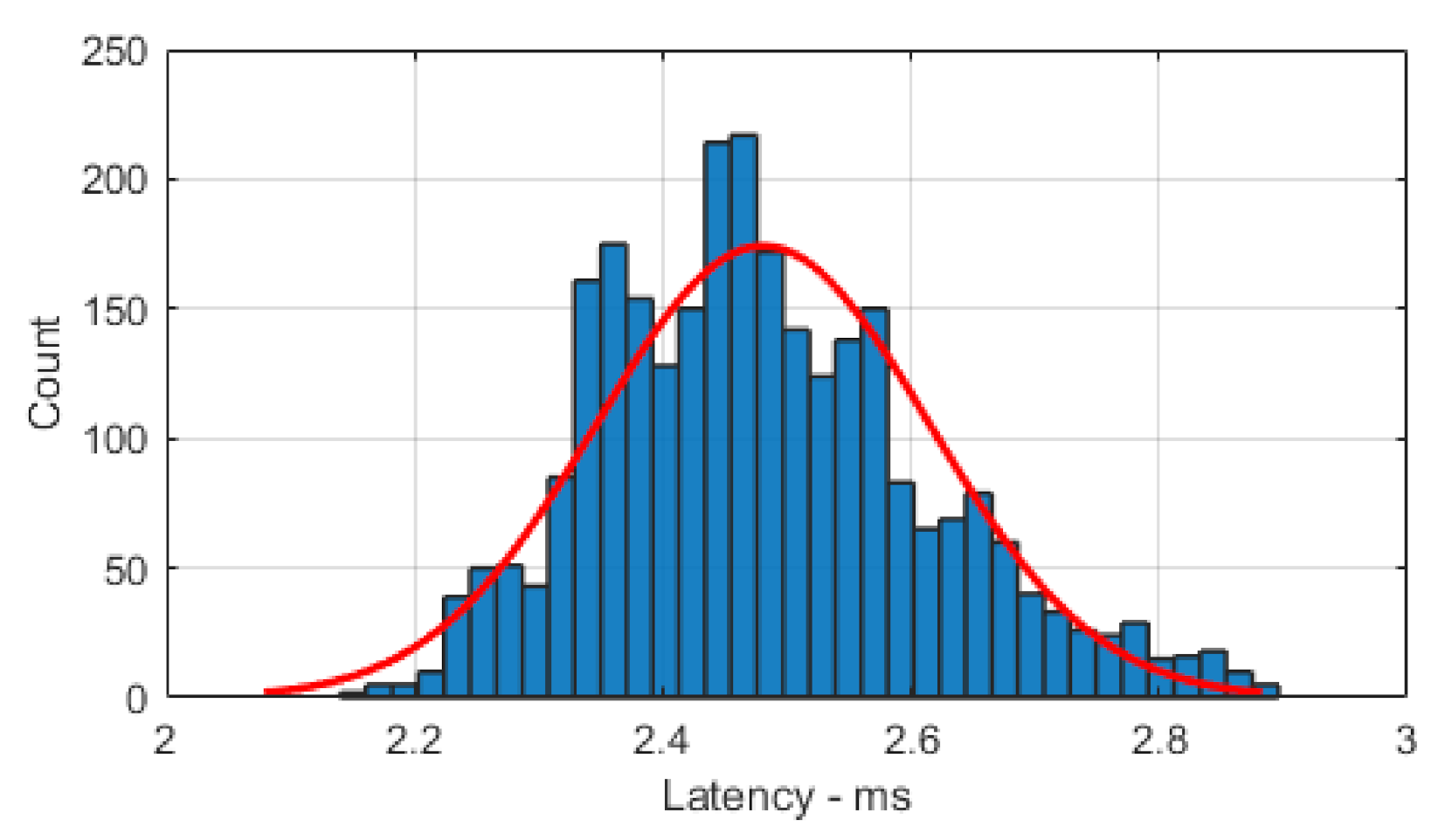
This section shows results on how the testbed could be used in collision avoidance, such as rear end collisions or emergency braking. This is based upon the latency finding of our experiments between sending and receiving nodes. Latency or information freshness is critical for CAVs as this is the speed at which the nodes are communicating information and is required to be 100 ms for standard BSM [39,40]. The latency that we monitored can be seen in Figure 1, and this experiment was conducted by measuring processing time and calculating the propagation time. The equation that is used to calculate End to End processing time (PT E 2 E ) is shown in Equation (1), and it shows the Time sent (T s ) and Time received (T R ) of a packet when transmitted through direct connection via SubMiniature version A (SMA) cable, which eliminates the propagation time. We then subtract the times from one another, leaving us with the processing time of both systems, which we assume is even on both sides. Then, we calculated the propagation time (T P ) for each distance, and, because we are only using distances up to 100 m, the propagation is at most 33.4 micro seconds. We then add the two times to find total End to End Latency (T E 2 E ). This latency, however, ignores the logical processing inside of the receiving device for reacting to the received packet, which would be negligible.
P T E 2 E = ( T R T S ) 2 T E 2 E = P T E 2 E + T P .
The results for latency can be seen in Figure 1 and are the product of over 2000 samples. We found that the latency ranged between 2.1 and 2.9 ms with a mean of 2.48 ms, showing the latency is lower than expected for information freshness of 50 ms required for pre-crash sensing [41].
To calculate the stopping distance (DS), we chose to use two different methods available and used in the literature. The first equation shown in Equation (2) is the most commonly used formula used in physics to calculate braking distance (DB); however, it is not based upon vehicle mass and assumes a rate of deceleration from 0 to max deceleration (maximum braking force) [35,36,37,38], where g is acceleration due to gravity (9.81 m/s2), V is velocity of vehicle, and u is the coefficient of friction. This equation is then used with an equation for thinking distance to calculate total stopping distance. Thinking distance (DR) is calculated with the velocity (V) and reaction time (TR). TR can also be represented in our case with TE2E when using the testbed.
D S ( m ) = D R + D B D R ( m ) = V T R D B ( m ) = V 2 2 g μ .
The coefficient of friction is a variable to describe the friction between the rubber tires of the vehicle and the road. Table 1 shows some road examples that are based on weather and ground type, with the average coefficient values associated [42]. In our experiments, we chose to use 0.8 as the coefficient of friction as this is the standard for normal dry road conditions for both asphalt and concrete.
The second equation shown in Equation (3) is used by many researchers, like in References [42,43,44,45], as this equation considers more in-depth variables concerning the type of car, road conditions, air conditions, and other parameters. Table 2 details each component of Equation (3), along with the value we chose to use and the range of values that are typically used. This is then added to DR, which is calculated in the same way as previously and leads to the total DS.
D B ( m ) = W 2 g C a e l n ( 1 + C a e V 2 η b μ W + f r c o s θ + W s i n θ ) w h e r e C a e = ( p A f C d ) / 2 D S ( m ) = D B + D R .
Using these equations, we predict the effect of using our maximum communication latency of 2.92 ms as the reaction time in place of the typical driver reaction time, which is suggested to be between 0.67 s and 2 s. The reaction time depends on driver state, such as age, driver experience, and state of mind. In this work, 1.5 s is chosen as the reaction time as this is the time reported by Brake to most accurately represent most drivers [46]. 
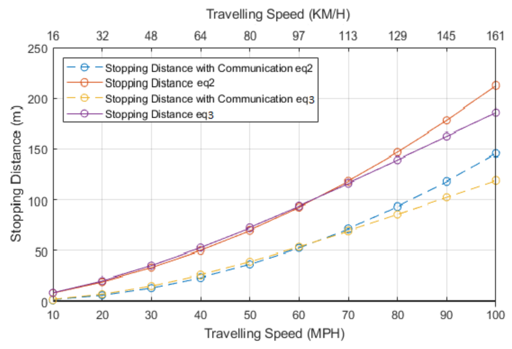
Figure 2 highlights the stopping distance reduction that could be observed when using communication-assisted systems or autonomous braking systems.
The results for this section show the difference between the stopping distance when using each method of measuring stopping distances, and they show the second has a slight reduction in distance needed. The second finding is that the reduction in distance is large when using the communication reaction time. This information can used in critical braking scenarios, such as debris on the road causing an emergency braking situation, a vehicle breaking down, a crash occurring, or sudden braking by the lead vehicle. Table 3 shows the distance that can be saved at each distance with the use of communication-based reaction time when the consecutive losses are 0. This table also shows the percentage of distance that is saved and at its lowest is a decrease of over 30%.
Through the use of the two formulas, it can be seen that Equation (3) is more accurate showing the braking distances for any vehicle that is chosen. Our experiments used a small hatchback, but the equation can be altered to represent any vehicle necessary. For these reasons, this will be the method used in our experiments.

4.2. Theoretical Model for Consecutive Losses

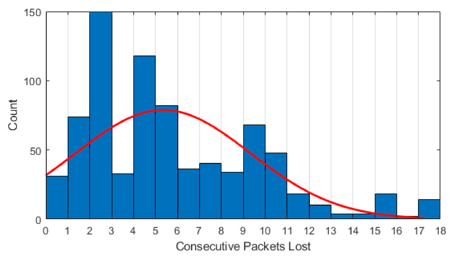
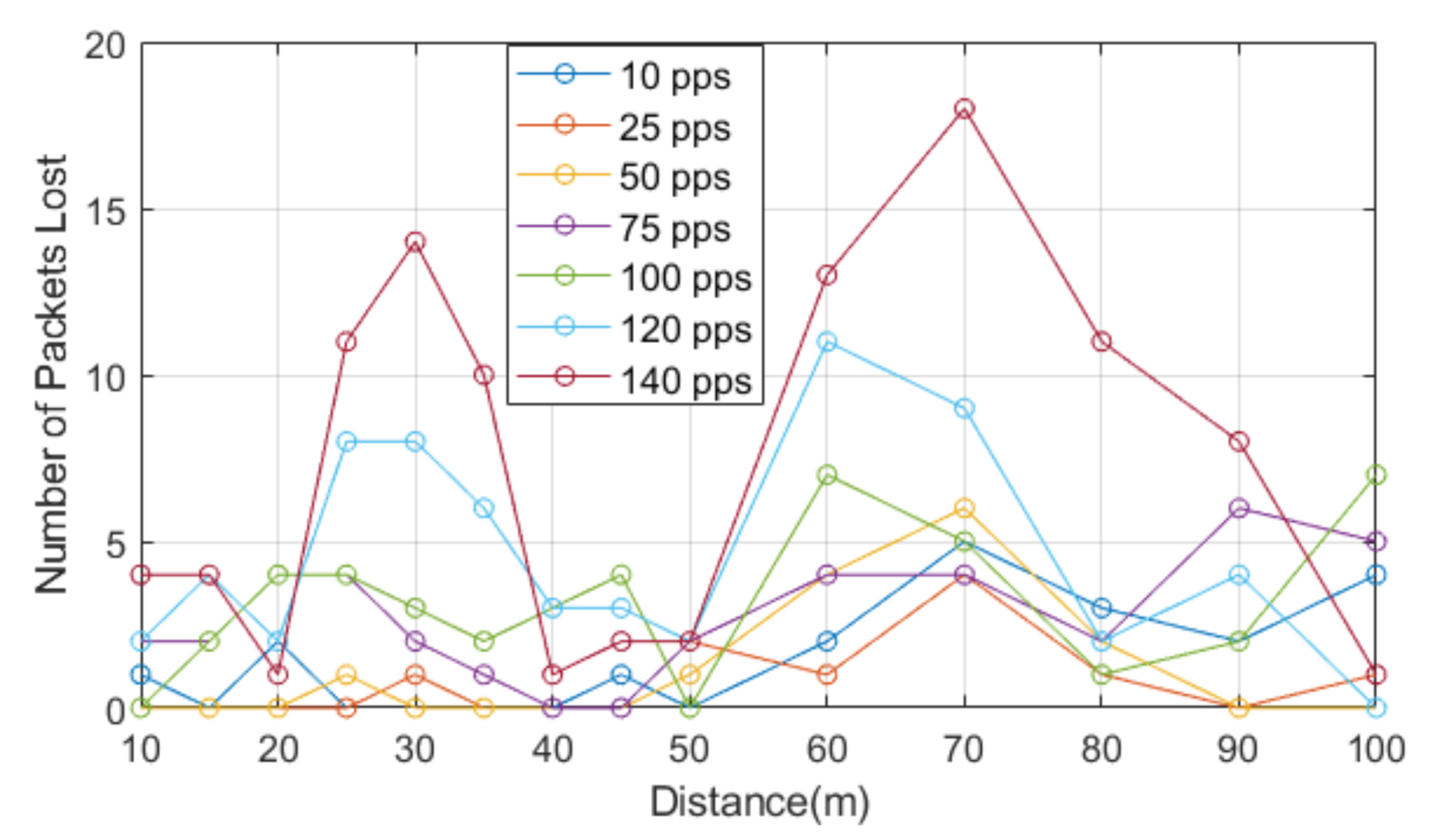
The following section outlines the main findings of the work, where the analysis is conducted as to multiple consecutive packet losses, and a model is designed and assessed to show impacts of consecutive losses. The losses we observed in our field tests, can be split into single losses or consecutive losses (burst losses). These types losses can occur due to circumstances, such as channel fluctuations, obstacles in the way, weather changes, or the hidden node problem. The use of UDP in our testbed means there is no acknowledgement of a packet being received, and this means that, if a packet is lost, the sender is not aware of this. UDP is the closest representation of a broadcast type communication used for CAMs/BSMs.
We believe this assists in identifying the reliability requirements for DSRC and highlights the importance of maintaining highly reliable systems. We have also chosen to monitor this over different data rates to analyze impacts by the Inter Packet Gap (IPG). The IPG will be abbreviated to T PI , which is the Packet Interval Time. The number of losses we chose to use will be shown later, but it will be stated that these losses are based upon real world field tests conducted.
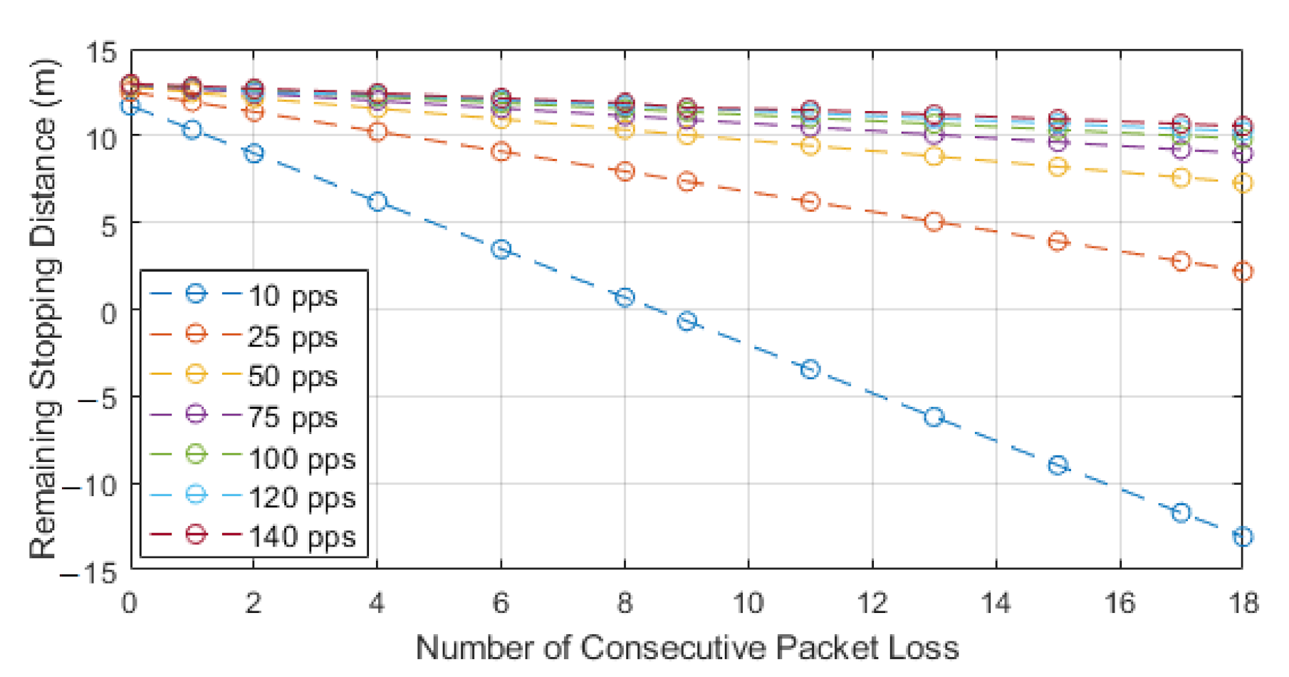
We developed a model that shows the theoretical loss on the stopping distance that consecutive packet losses could have. This model is based upon the field work for stopping distance, along with an equation that calculates the loss of stopping distance per packet, which includes the packet sending interval. Equation (4) shows the model formula, and Table 4 shows the parameter information.
R S D = ( T E 2 E V ) + W 2 g C a e l n ( 1 + C a e V 2 η b μ W + f r c o s θ + W s i n θ ) V [ P a L ( T E 2 E + T P I ) ] .
This initial model represented in Equation (4) does not consider the next packet after the burst loss being received and processed. This means that, after consecutive packet losses, no packet is successfully received, processed, and an action taken. This would be vital in autonomous systems, whereby the communication would be essential to maintaining adequate distances and awareness. For this an extra iteration of processing, round-trip time and packet interval would need to be included, which are used to represent the packet being received successfully, and this is shown in Equation (5).
R S D = ( T E 2 E V ) + W 2 g C a e l n ( 1 + C a e V 2 η b μ W + f r c o s θ + W s i n θ ) V [ P a L ( T E 2 E + T P I ) ] + V ( T E 2 E + T P I + P T E 2 E ) .
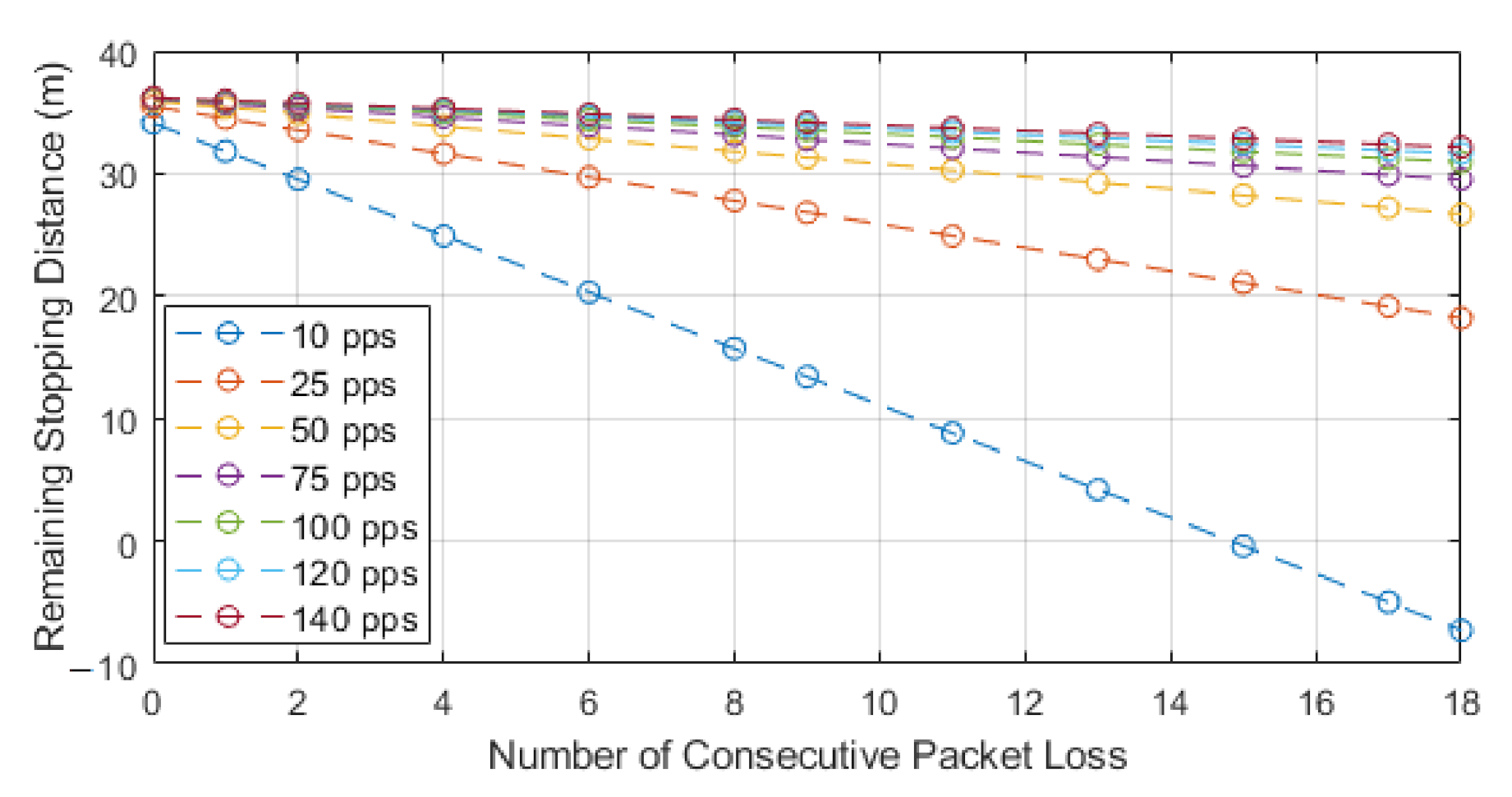
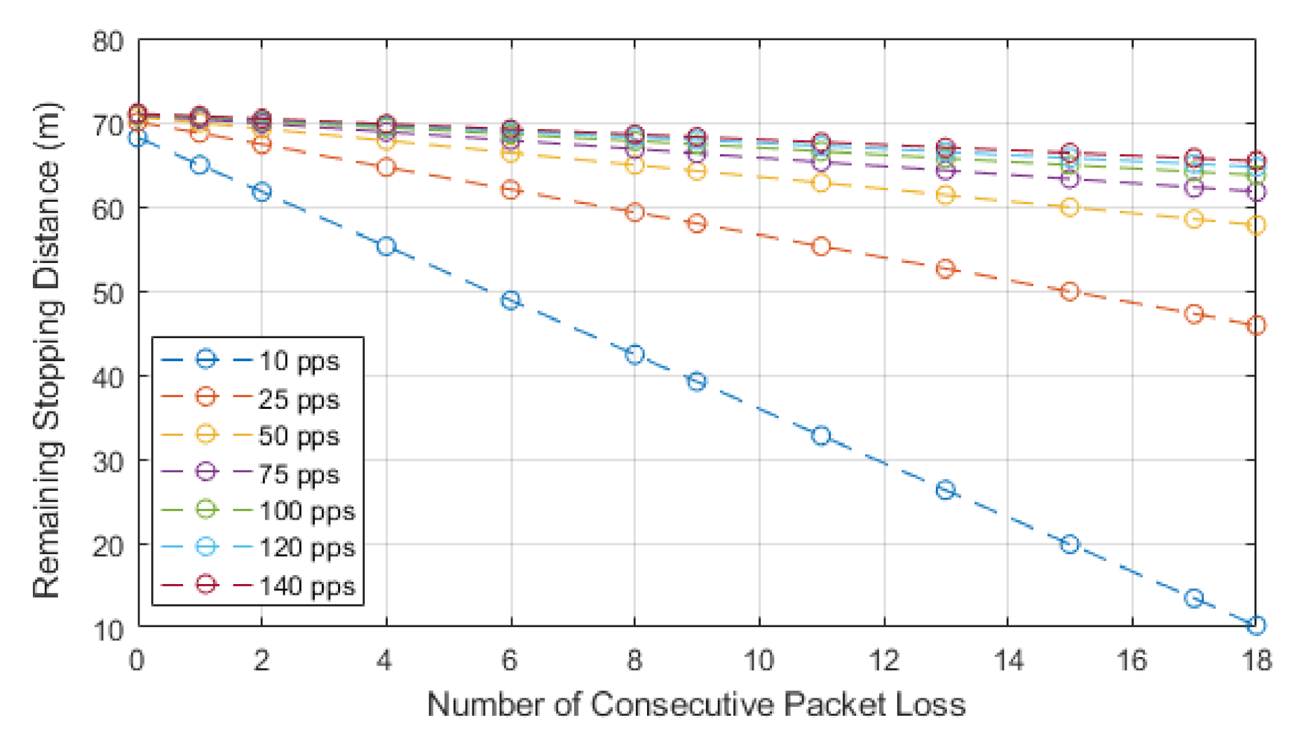
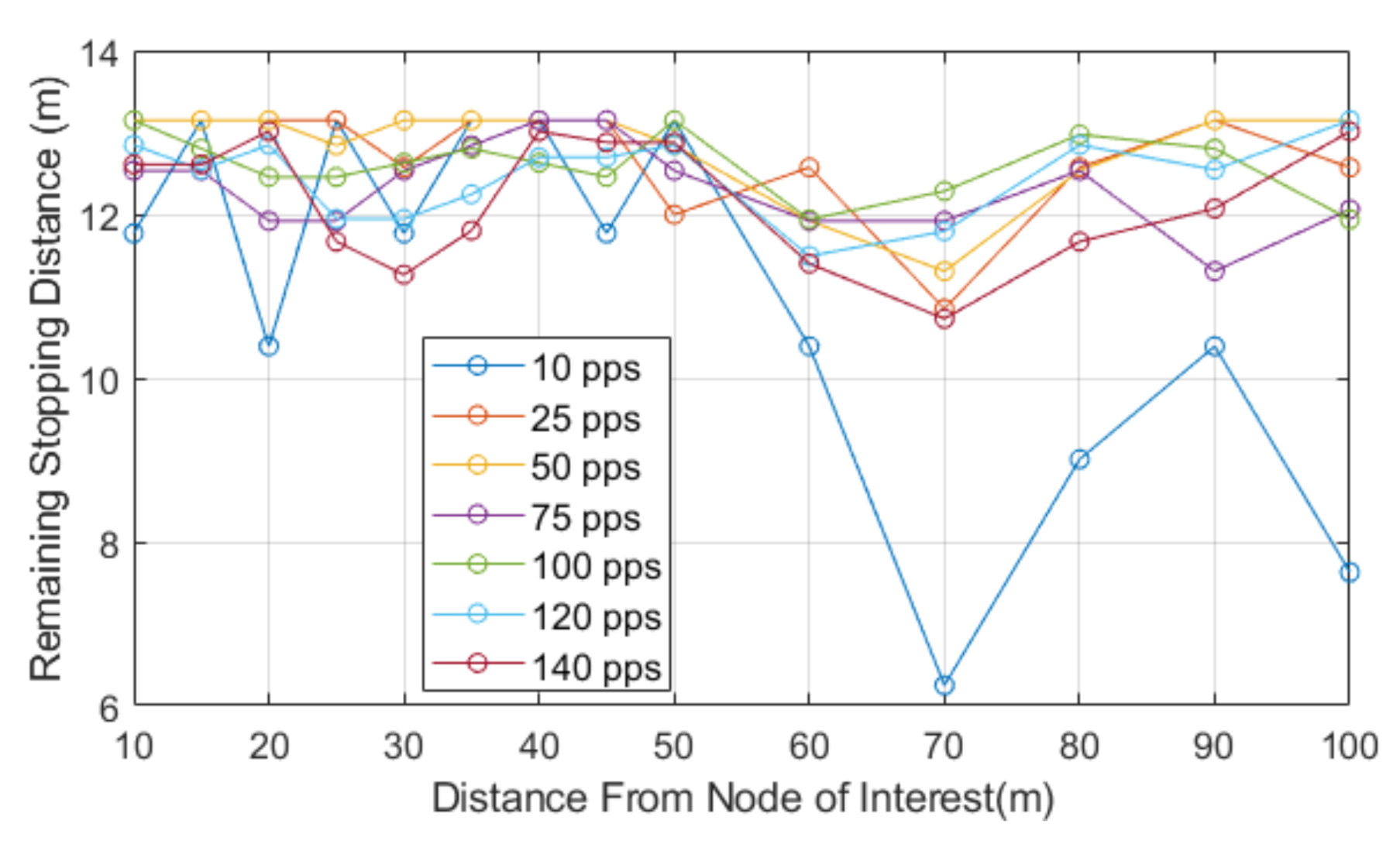
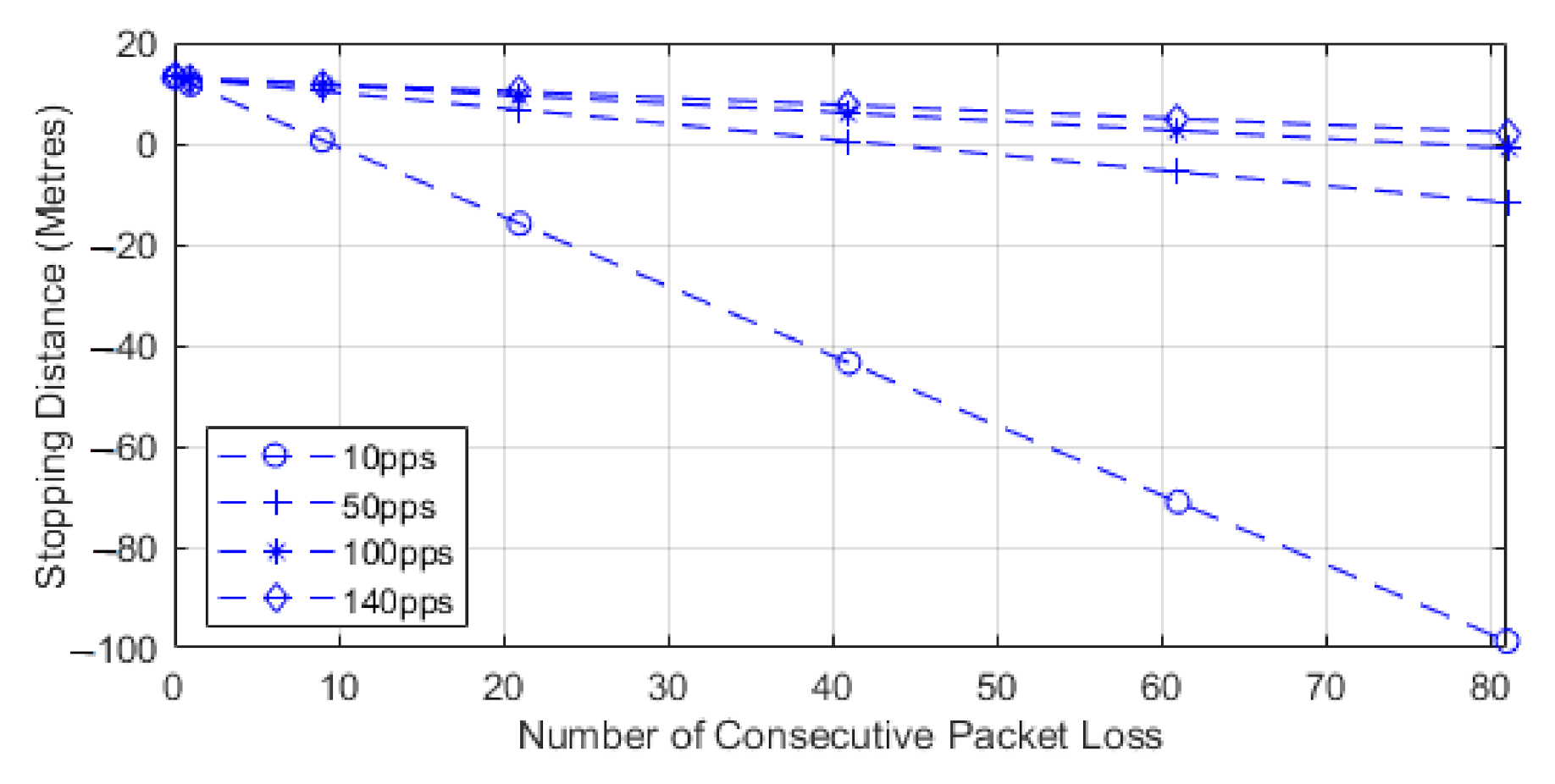
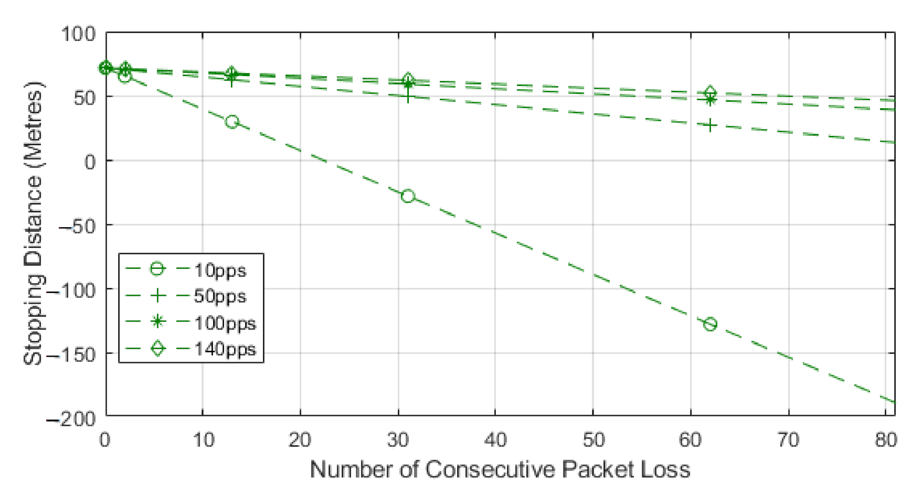
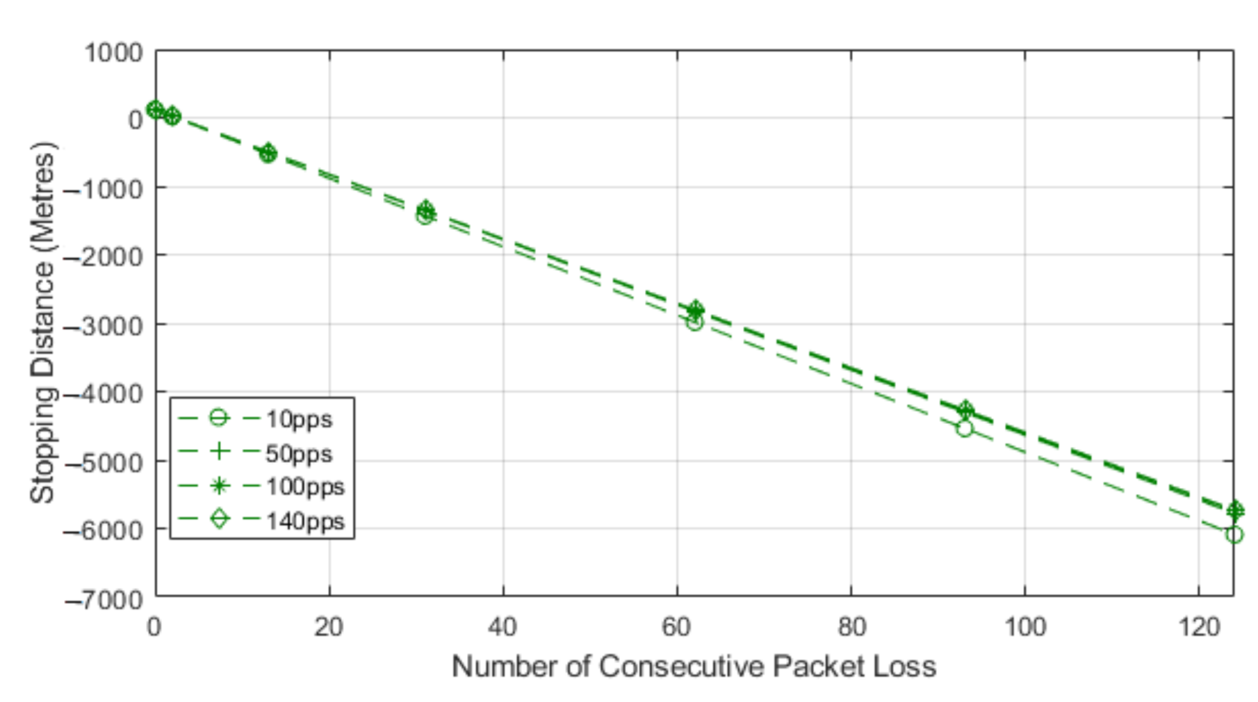
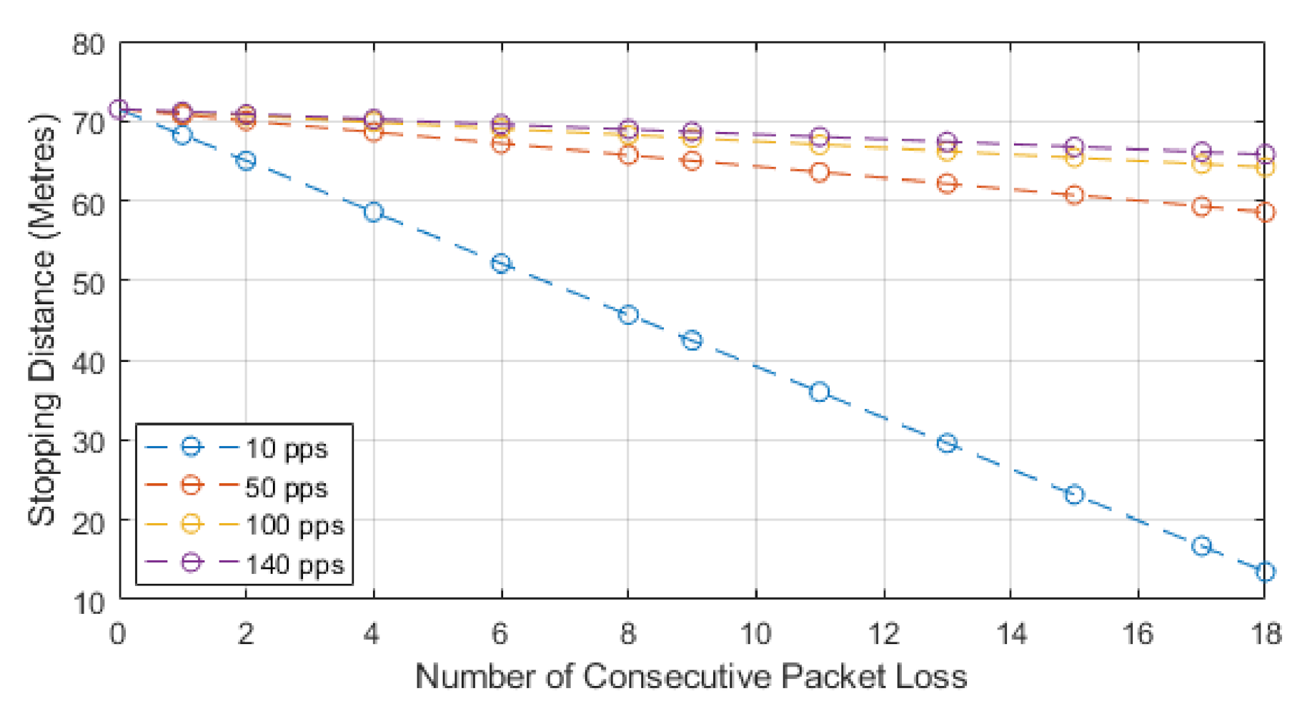
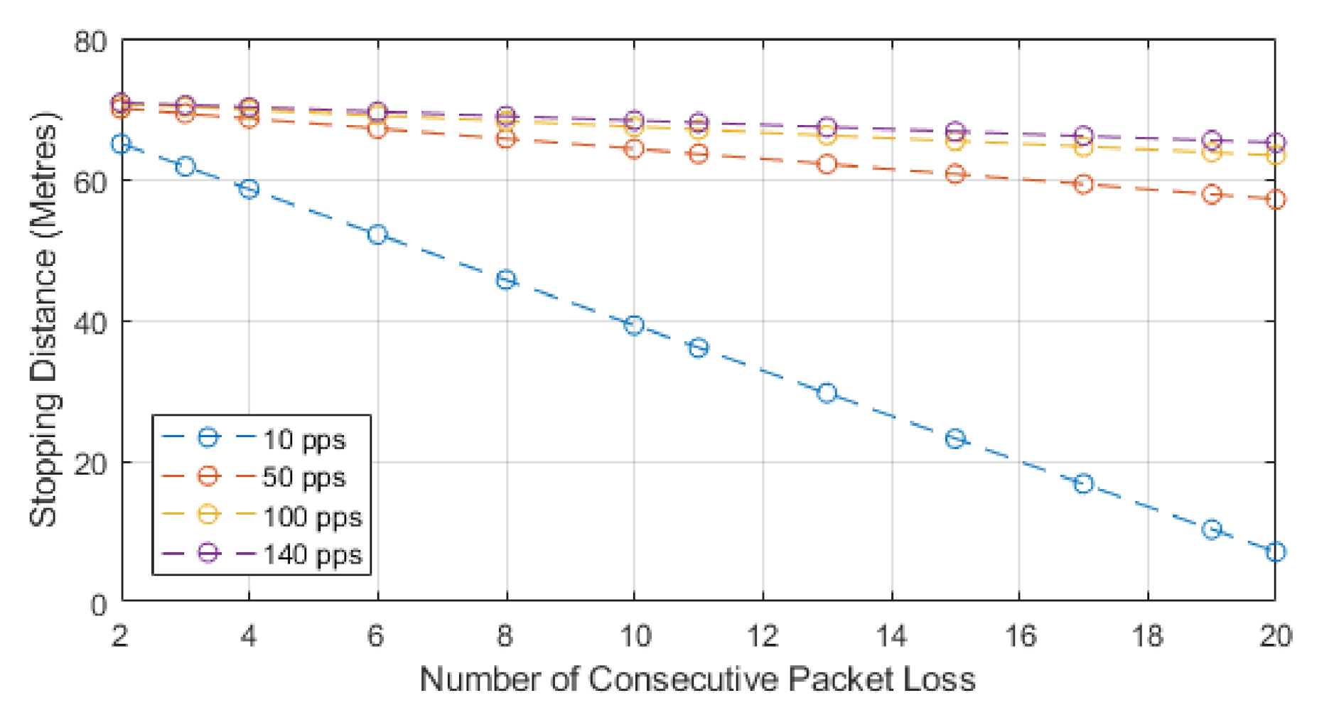
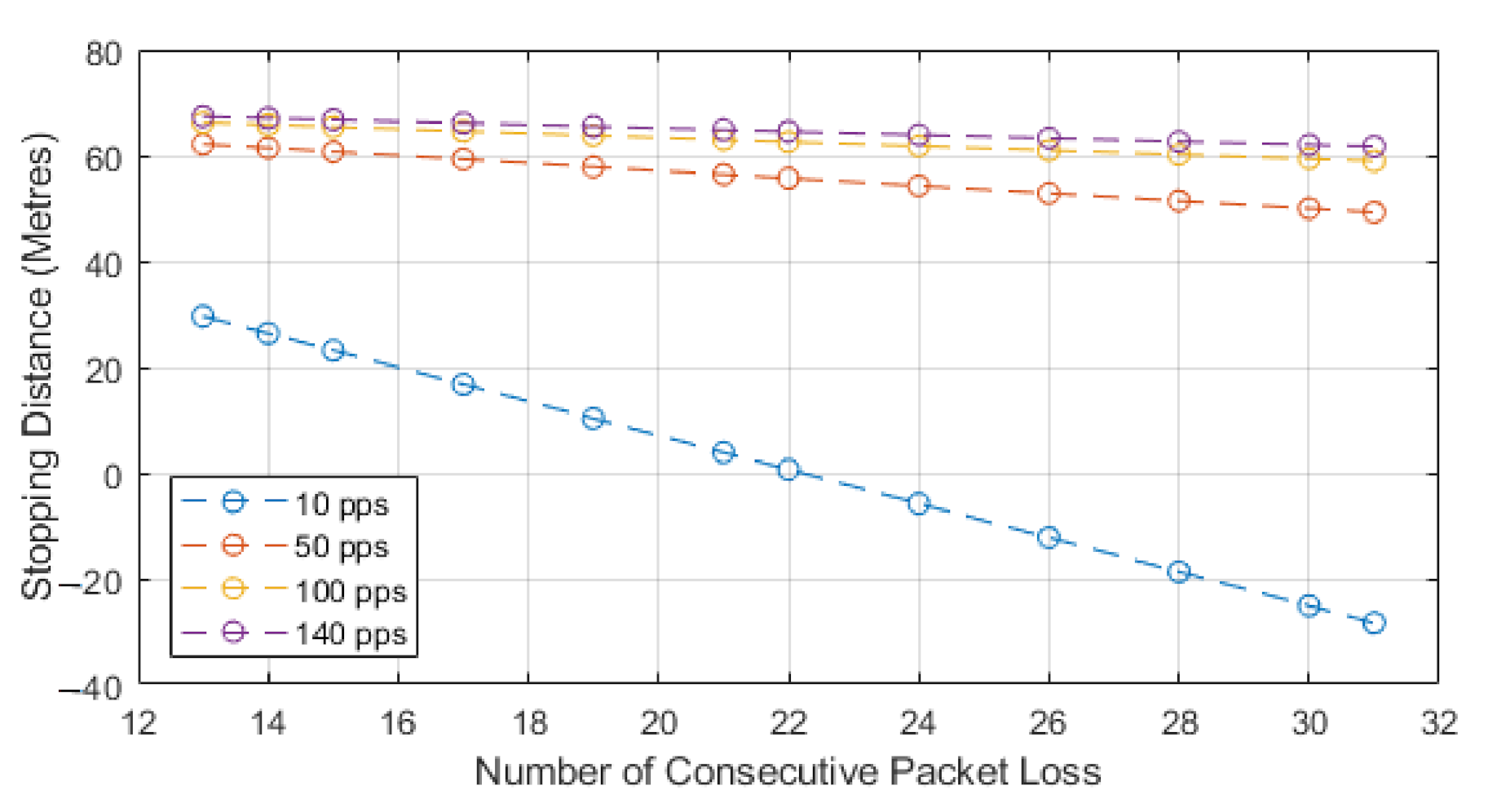
We chose to use the second model as this paper is focused on the impacts of how packet loss can alter the stopping distance when relying on communications, and this equation highlights that impact. The model works by utilizing Equation (3) to find the normalized stopping distance for a vehicle and then we subtract the distance lost via consecutive losses. The losses can be seen in the second part of Equation (5). The result of this equation will leave us with the distance remaining to a collision or stopping distance remaining. We know that, after losing the consecutive packets, the vehicle will still need to stop in order to show the full distance required to stop, and the Equation (5) sign could switch. This would then represent the stopping distance, plus the distance lost through consecutive loss, to leave us with total stopping distance. In our case, we are showing how lead and following autonomous vehicles communicate, with the following vehicle adhering to a communication-assisted stopping distance. We then analyze how this stopping distance is impacted with the addition of consecutive packet loss, and this is shown for different speeds and data rates. For our results, we show the stopping distance when 0 packets are lost, and we then show how the stopping distance is reduced with each consecutive loss. This highlights how the reduction in reliability leads to reduced stopping distance and, hence, a higher chance of collisions with the lead vehicle. As the reduction value reaches 0, we deem this to be the point at which lead and follow vehicle will be occupying the same space or that a collision may have occurred. We also show a negative value, which would mean the follow vehicle has gone past the lead vehicle, and this would be classified as a collision; we show this to identify the impact of reliability.

5. Simulation of Field Tests

We chose to analyze our results in two different ways: the first is a distance independent instance, where we theoretically analyzed what would happen with a consecutive loss of packets, and this will range from our lowest to our highest. The second is a distance dependent analysis based on the packet losses we measured during field tests, at each distance up to 100 m. Both scenarios are measured at various data rates and traveling speeds.

5.1. Distance Independent Consecutive Packet Loss

To measure the distance independent losses, we used our testbed to monitor the number of consecutive losses observed in 3000 experimental samples when measuring packet loss rates. To do this, we attached a number in each packet and extrapolated the number, and this allowed us to see the number of packets lost consecutively. We chose to do this over a 100-m distance because typical stopping distances up to 70 mph fall within this distance range. We took our samples and compiled a normal distribution plot showing our spread of consecutive losses. This can be seen in Figure 3 and shows most consecutive losses are in the range of 1–11. It can also be seen that the most common occurrence of consecutive loss is 2 packets, and the mean is approximately 5. Using these results, we selected a range of values through 1–18 because 1 is our minimum consecutive loss and 18 is our highest. We produced results for 30 mph, 50 mph, and 70 mph and conducted this over the full range of data rates we utilized in our testbed, i.e., 10 to 140 packets per second.
Table 5 represents the remaining stopping distance available after a number of consecutive losses at 30 mph and 10 pps. The table is used to give an example of what the results look like after applying our model.
As can be seen at 0 losses, this is the full stopping distance required at 30 mph. The distance shown on the right is the remaining stopping distance that would be available after consecutive loss, shown on the left. The results for 11 packets and higher show a negative value. This negative value means the distance remaining to stop has reached a point whereby a vehicle could have collided or overtaken the lead vehicle. This highlights the importance of reliability for communication when autonomous vehicles become more widespread. There are variables in the model, and, in these tests, the three variables are:
  • Consecutive Losses, which have been set to—0, 1, 4, 6, 8, 9, 11, 13, 15, 17, 18;
  • Data Rate in packets per second, which is configured as—10, 25, 50, 75, 100, 120, 140; and
  • Speed in mph or (km/h), which is configured as—30 (48.27), 50 (80.45), 70 (112.63).
The following set of figures are used to show the results for distance independent measurements, and these are for each speed and data rate. Figure 4 shows 30 mph, Figure 5 shows 50 mph, and Figure 6 is for 70 mph.

5.2. Distance Dependent Consecutive Packet Loss

A second scenario to be analyzed is the impact of distance dependent packet losses. This scenario is based upon the studied vehicle being at different distances from the vehicle of interest. In this case, we measured how the stopping distance is reduced when vehicles are at different communication distances. We first show Figure 7, where we can see the receiver power over distance from 0–250 m. Figure 8 is used to show the number of packet losses at each distance and data rate. It can be seen in this figure that, at distances of 30 m and between 60–90 m, there is a spike in packet losses at the 120 and 140 pps curves. We can refer to Figure 7, where we see that, due to the fading nature of the channel, the received power suffers degradation over these distances, and we can attribute the number of packets being transmitted that cause this fading to have a larger effect of the reception percentage.
Following from the figure used to show the packet losses at each distance, we can then show how consecutive packet losses will impact stopping distance based on real world distance dependent packet losses measured. We utilized our developed formula and applied it to the field test measurements at each distance. Figure 9, Figure 10 and Figure 11 show the stopping distance when the vehicle traveling has a velocity of 30, 50, and 70 mph and is again shown for each instance of data rate. In these figures, we observe that the 10 pps plot has a large reduction in stopping distance from a distance of 70 m, and we can attribute this to being caused by the fading effects mentioned previously, as observed in Figure 7 and Figure 8.

5.3. Analysis of Distance-Based Results

The results from our experiments show that the usage of communication can assist with the reduction of stopping distance, enabling a reduction of up to 30% when packet losses are 0. However, for the consecutive losses, we can see an impact in both distance dependent and distance independent cases.
Our results show that, at all speeds, consecutive packet loss leads to a reduction in stopping distance. We can also see how important data rate is for vehicle communication, as at each instance of 10 pps for 30 and 50 mph shown in Figure 4 and Figure 5, a negative value is produced indicating the stopping distance has reduced below 0. This means the following vehicle has either collided with the lead vehicle or overtaken it.
Figure 4 shows the results for 30 mph and shows the data rates of 120 and 140 pps have a reduction of less than 5 m, which is the average length of a vehicle, hence leaving two vehicles space still available to take emergency action. When considering the maximum consecutive packet loss, the minimum data rate that would provide adequate time to respond would be above 75 pps per second in the 50 mph experiments, as seen in Figure 5. Anything lower than this and the stopping distance is reduced by between 50–75%. In the 70 mph example in Figure 6, 25 pps would have a reduction of less than 40%, and the higher data rates with consecutive loss degrade the stopping distance by approximately 10%.
We can draw a conclusion from our results that, at lower speeds, the consecutive packet loss has much more of an impact. This is due to the stopping distance being smaller, therefore giving less distance to receive the delayed communication message. However, due to high speeds, if packets are not sent at a high enough rate the stopping distance is reduced too low for adequate reaction. This leads to less time for an action to be made, but we also show that this can be mitigated with high data rates.
The main conclusion to be drawn from the distance dependent test is that, in order to mitigate the effects of consecutive losses, high data rates must be used in order to provide adequate reaction time. We can also see that, if the requirement of a 99.9% reliable system is adhered to, that, in all tests, a loss of two packets consecutively has minimum effect in Figure 9, Figure 10 and Figure 11. We can also see that the lower data rates suffer more at higher distances but cause more significant degradation to stopping distance at lower distances; the primary example of this can be seen in the 30 mph tests in Figure 9. It can also be seen that, as the distance increases, the packet losses have less of an impact exponentially.
Figure 7 can also show the reason that the packet loss suffers somewhat at lower distances. The figure shows received power levels at distances up to 250 m, but our focus is only to 100 m. It also shows the fading characteristics indicated at the lower distances by the rapidly changing power levels, hence having the higher losses seen at lower distances. Figure 7 also highlights the power levels for lower distances suffer fading, but 100 m has a lower power level and yet does not suffer the same level of packet losses. This can be attributed to the fading characteristics of the channel and the gain settings on the SDR; we can also see that, at 60 m, a significant level of fading is observed.

6. Simulation of Density Losses

The following section is now focused on the connotations of losses incurred by the density of the vehicle network. Simply put, this is analyzing the number of losses caused by an increase in the number of vehicles transmitting simultaneously.
This is essential towards analyzing the losses incurred in vehicular networks and how the reliability can be hindered by large amounts of nodes broadcasting their individual safety messages and how the dissemination of messages can reduce reliability. Our approach to this was to simulate a vehicular scenario based on number of nodes within communication vicinity and relate this to packet losses and safety distance. These experiments prove that the use of communication will reduce reaction time, and, due to this reduction, both nodes in communication range and safety distance are reduced.

6.1. Density-Based Losses

In this section, we use a simulation to monitor packet losses when considering multiple nodes in a 3-lane highway environment. We assume to eliminate the opposite flowing traffic with the use of location-based broadcast, which is the preferred method for Cooperative Collision Avoidance (CCA) [47]. Our initial calculation is to approximate the number of nodes within broadcast communication range. We choose to incorporate the use of Automatic Gain Control (AGC), which is used to alter the gain depending on the speed being traveled. Lower gains can be used at lower speeds to have a smaller communication range.
The first step of this is to identify the communication range, which will be known as the safety distance. The safety distance is approximately the same as the reaction time for a human driver or DSRC/Advanced Driver Assistance Systems (ADAS) device, which, as we have mentioned, is approximately 1.5 s without the DSRC testbed and 2.92 ms with the testbed. For the consideration of safety distance, we do not use the separate measurement of braking distance. As we described previously, stopping distance is the combination of braking distance and reaction distance. In this scenario, reaction distance is essentially the safety distance, and we are calculating the minimum required gap between vehicles depending on the speed being traveled. When using a full ADAS system, an adequate approach must be made for the calculation of braking distance because, without this chain reaction, accidents would be prevalent. This is merely a simulation to represent an example for the safety distance with communication and the impacts of node density.
It can be shown that the distance traveled in the reaction time (Safety Distance or D s ) is directly affected by: the time taken for a reaction to be made by the driver (T R ) and the acceleration of the vehicle being driven (a). This can be shown in Equation (6) as:
D s = a T R .
In the case of the testbed reaction time, we must also consider a delay within the system due to the processing of the information and the mechanical delay of activating the brakes. We will assume this to be equal across all acceleration speeds and have set this value as 0.25 s, and it will be specified as Reaction Processing Time (T RP ). This is shown for human driver in Equation (7) and ADAS in Equation (8).
D s , h = a T R ,
D s , a = a ( T R + T R P ) .
The difference between the two safety distances according the traveling speed can be shown and in addition, we also show the results of various stopping distance algorithms. These algorithms will be the Mazda Algorithm [18], the Stop Distance Algorithm (SDA) [18], and a more recent variant, known as the PATH (Berkeley) Algorithm [18,27,48]. The PATH algorithm is a modified version of the Mazda algorithm and is used to show safety distance calculation or critical warning distance.
In order to show the various algorithms, the deceleration of a vehicle is assumed to be at maximum for both following and leading vehicle. This is taken from a study conducted into various vehicles [48,49], and, for our interpretation, the deceleration rate for a standard Petrol car is used. This can also be calculated using a deceleration formula and the initial calculated braking distance without the use of Reaction time.
Deceleration ( a ˙ ) can be calculated in two different methods: with S f representing final speed, and S i representing initial speed, t denotes time, and d is distance.
a ˙ = ( S f S i t ) ,
a ˙ = ( S f 2 S i 2 2 d ) .
For this scenario, Equation (10) is used as the braking distance has already been calculated. The deceleration will then be modeled to represent the rate of deceleration ( a ˙ R ). This is taken from a work by Woo et al. [48] and is a validated model representing the reality of braking via CarSim simulator. The formula Equation (11) is a linear equation representing an approximation of deceleration rate and is used in order to simplify the vehicle braking dynamics, where a ˙ is the max rate of deceleration, and the mechanical delay is (T RP ).
a ˙ R = a ˙ T R P

6.2. Safety Distance Algorithm

With the deceleration rate model now described and in addition to the calculated Human reaction safety distance and the ADAS reaction safety distance, the algorithms previously mentioned will be briefly explained and shown;
Mazda algorithm is a worst-case scenario to ensure collisions do not occur and is shown in Equation (12), where v l , v f , v rel represent leading, following, and relative vehicle velocities, and ( a ˙ f ),( a ˙ l ) represent deceleration. This algorithm assumes that the two vehicles are at a constant velocity and that, at T 2 , the leading vehicle will begin braking at the deceleration rate specified, and that the following vehicle will begin braking after T 1 at its own deceleration rate. R min Is used to represent a minimum range or a tolerance rate.
D s ( v l , v f , v r e l ) = 1 2 [ ( v f 2 a ˙ f ) ( v l 2 a ˙ l ) ] + v f T 1 + v r e l T 2 + R m i n .
SDA follows approximately the same idea as Mazda; however, it is based on the difference between the two stopping distances of lead and following vehicle, and it is usually a part of ADAS that utilizes driver warning systems. In this algorithm, T R represents the reaction time of the driver. This is shown in Equation (13).
D s ( v l , v f ) = v f T R + ( v f 2 a ˙ f ) ( v l 2 a ˙ l ) .
PATH is a modified version of the Berkeley algorithm and is based upon two vehicles, where the lead vehicle begins braking, and the follower reacts after T r and begins to brake. This algorithm also uses R min to represent a minimum range or a tolerance rate and is shown in Equation (14).
D s ( v l , v f ) = 1 2 + [ ( v f 2 a ˙ f ) ( v l 2 a ˙ l ) ] + v f T r + R m i n .
In these algorithms, we will assume that the vehicles velocity and deceleration are the same; therefore, the relative speed will be 0. The Berkeley example will also be used with both the deceleration value calculated from our simulations and the industry standard value of 6.44 m/s 2 [50,51]. The final method to be analyzed in the Highway Code guideline of a 1 m per every mile per hour [52,53]. For instance, at 30 mph, the gap should be left is 30 m safety distance. We found that, after calculating with each algorithm, the SDA, PATH, and Mazda equate to the same safety distance as the finding we made for human-based safety distance. For this reason, we will only plot five variations of safety distance, which can be seen in Figure 12. This graph highlights how much quicker the ADAS-based braking system would react compared to a typical human reacting to a warning produced by the other algorithms or from a visual reaction from eyesight.

6.3. Node Density Simulation

With the safety distance calculated, the number of nodes in range can now be predicted for each traveling speed. This will be based upon the calculated safety distance and 5 m set as a car length.
Due to the use of omnidirectional antennas, it is known the radiation pattern is a circle with the center point being the antenna. To communicate to vehicle of interest, the radius will be the safety distance plus one full car length. As this is a circle pattern, the diameter is simply shown Equation (15). However, we also know that a vehicle is approximately 5 m, and a centrally placed antenna would limit the circumference; to compensate, we add an additional 5 m to the diameter to represent the vehicle of interest, shown as VL. This equation will only be applicable in our simulation as we are only considering average vehicle sizes, and, to more appropriately represent other vehicles, such as a bus or lorry, a custom radius distance would be applicable.
d = ( r 2 ) + V L .
With the diameter calculated from the safety distance, we can now predict the number of nodes within this diameter. For example, at 30 mph and using the PATH, safety distance of 20.2 m is 45.4 m. We then calculate how many nodes will be present in the communication range. This can be simplified down to number of cars per lane, safety distance per car, and the number of lanes to give an approximate minimum value. For our number of nodes, we consider all vehicles maintaining the 20.2-m spacing, with an approximate length of 5 m per vehicle. Therefore, in one lane of traffic, two nodes will be within range. This will be then multiplied by number of lanes, leading to the classification that 9 nodes will be within range, including the central node. This is, however, the best-case scenario; a worst-case scenario would be that the minimum safety distance is not adhered to, and cars could be packed tightly together. This leads to 11 cars per lane being within communication range, which results in a total of 33 at 30 mph. This is shown in Equation (16) for best case and Equation (17) for maximum nodes, where d represents diameter of communication, r represents radius of communication, L is used to show number of lanes, and dc shows length of vehicle.
N o d e s a v g = ( ( d / ( r + d c ) ) + 1 ) L ,
N o d e s m a x = ( d / d c ) L .
Figure 13 shows the result of the node calculation, and it shows that the ADAS has a vastly reduced number of nodes in communication range due to the reduction in reaction time compared to that of all human reaction-based analysis. As mentioned, PATH and human reaction are identical and so will be treated as the same for the simulation; this can also be seen in Figure 13. The worst performing is the general guidance given by the highway code, and we can deem this to be because it is rather a guideline than an effective algorithm. It should also be noted that the human reactions are not due to the emerging situation but rather the reaction to the ADAS warnings provided by DSRC, whereas the ADAS reaction is a reaction based on automatic braking provided by DSRC. The figure also shows the losses scale by miles per hour with changes only occurring in incremental steps. This is a highly useful finding for the use of automatic gain control, as the diameter would be kept identical until a threshold to change to the next limit.
As the number of nodes are now calculated for each speed, a simulation can be performed to find consecutive losses. The simulation has been conducted using MATLAB and is a representation of communication between DSRC nodes competing for channel access. The simulations have been performed with varying numbers of communicating nodes to represent the number of nodes in communication range for each traveling speed. The simulation provides the number of expected consecutive packet collision probability per node density/traveling speed, when all nodes are competing for channel access with BSM messages being broadcast.
The simulation is based upon node density over DSRC communication and contains the parameters used in DSRC for MAC configuration. This includes collision window timings, slot allocation, and acknowledgements for packet reception having been removed. These settings have been gathered through various sources [29,54,55,56]. Further information relating to the simulation and the settings have been collated from References [56,57], and these relate to data rate and transmission scheme. The simulation has kept as many variables the same as the tests in the distance-based experiments to maintain consistency, comparability, and compatibility. The acknowledgements for packet reception have been removed. Table 6 is used to emphasize important simulation parameters we used.
We chose to display only ADAS results as we will be using this to compare with the results of distance-based losses. Figure 14 shows the probability of consecutive packet collisions for the node of interest when a specific number of nodes are within its communication range. We can see from these results that the number of losses due to density is more severe than those of distance-based. The DSRC system suffers up to 15% losses, which is approximately 150 packets with 21 nodes in range. When compared to the distance-based, we saw a maximum loss of 18 packets. This highlights the importance of the capabilities of the network in terms of traffic load and an adequate allocation scheme to reduce these losses in order to meet stringent requirements for safety. We will show the linear regression curve equations produced that enable the calculation of number of packets lost due to collisions, for each different safety distance algorithm, and each will be shown individually in Equations (18)–(21), where x represents the number of nodes.
A D A S = 0.72 x 0.57 ,
P A T H = 0.57 x + 1.8 ,
P A T H I S = 0.54 x + 2.9 ,
H C = 0.49 x + 4.7 .

6.4. ADAS/DSRC Losses

In order to show comparable results to the distance-based experiments, we will need to show the number of consecutive packets lost at each traveling speed. To do this, we use the linear regression formulas we developed thorough the simulation and apply them to the number of nodes in communication range found in Figure 14. These calculations will be shown up to 100 mph, and the values can be seen in Table 7 for each algorithm.
Table 7 shows packet losses due to density collisions are much higher than those of distance-based, primarily due to nodes competing for transmission time slots. The table shows the number of consecutive losses per 1000 packets for each algorithm, with 100% losses being shown as per our linear equation, and the ADAS losses can be seen to be 124 at 70 mph. This level of loss is considerably high for successive packet collisions. For this reason, we will produce a scale showing 1–100% losses recorded as consecutive. Figure 15 shows the results from extrapolating the distance and packet losses based upon traveling speed. Table 8 shows the corresponding packet loss value to each percentage for clarification, and these have been rounded to the nearest whole packet.
The results will now be shown as stopping distance reduction, with the delays caused by each consecutive packet loss percentage. This will be shown for 30, 50, and 70 mph respectively and will use three different data rates, 10, 100, and 140 packets per second. The algorithm used for calculating stopping distance in previous experiments are again utilized here; however, we now use the altered packet losses from density in place of the distance-based. Figure 16, Figure 17 and Figure 18 show the results of this simulation.

6.5. Analysis of Density-Based Results

The figures provided show similar results to that of distance-based losses. However, we can see that the losses are far greater; thus, the distance needed to avoid potentially dangerous collisions is vastly reduced in comparison. As DSRC aims for 99.9% reliability, our most appropriate result is seen in the 1% category or 1–2 packet losses. If the losses are kept at this level, the stopping distance would not be affected, but, as the losses increase to even 10%, we can see that a rate of 10 pps is unsafe to use. The use of 140 pps performs well at 70 mph, but, at 30 mph, the 140 pps becomes unsafe to use; this also shows that DSRC needs to have high data rates if the reliability is reduced below 99%.
In order for brief comparison, Figure 19 shows the PATH reaction at 70 mph and has the reaction time set to the standard human reaction as used previously of 1.5 s. This figure is only an example used to show how much DSRC systems can assist and reduce stopping distances. It is acknowledged that the human driver would react from visually witnessing an emerging scenario; therefore, the figures are highly improbable. The only loss percentage that would not suffer significant degradation is at 1% consecutive loss.
These tests highlight the importance of three main factors; reliability, data rate, and latency. Other services would be able to cope with the loss of any of the three, but, where safety is concerned, they are all of vital importance and must be ensured to the highest of levels.

7. Joint Distance and Density Losses

The final part of our analysis is to employ a joint loss system between both distance reliant and density-based losses. This will be a brief comparison as we know that density losses contribute significantly more to losses than those of distance. To do this, we took both previous results for distance independent losses and the density-based losses and combined them in four different scenarios. These scenarios are all shown at 70 mph and for four different data rates of 10, 5, 100, and 140 pps. The 4 differences used in each simulation are 0%, 1%, 10%, and 100% of the density-based losses. The algorithm used is the same as with distance independent; however, we modified it to consider two different packet loss scenarios. The results can be seen in Figure 20, Figure 21, Figure 22 and Figure 23.
From the figures produced, it can again be seen the biggest contributor to unsafe stopping distances is at any point over 1% density-based packet losses, and the second highest is the use of low data rates, such as 10 pps. In the 10% and 100% figures, the only data rates that do not become unsafe are those of 100 and 140 pps, and this is where the stopping distance does not decrease highly, further proving the requirement of high data rates. The 10 pps performs extremely poorly when subjected to high density collisions, which would be expected.
The final point to note is that, with the requirement of 99.9% reliability, our examples at density 1% and maximum distance loss of 18 packets consecutively, which totaled approximately 20 consecutive packet losses, 140, 100, and 50 pps, did not approach unsafe levels of distance.

8. Conclusions

This paper investigated how important reliability is in the context of vehicles and safety, especially in the context of stopping distances. We analyzed real world field test data and showed how highly reliable communication could assist and even shorten the stopping distance via the significantly reduced reaction time. We observed that autonomous or automatic braking systems will be a lot more efficient in reducing stopping distances, which in turn will allow for more efficient traffic. A model for calculating the reduction to stopping distance when subjected to consecutive losses has also been produced and quantified, and this helps to highlight the importance of reliability when a system is based solely on communication. Our results also showed that almost perfect packet reception must be guaranteed for safety when CAVs become more prevalent on the road, whilst also showing that lower data rates are not suitable for all safety needs.
We also proved that a method of reduced safety distance with the use of our system can reduce the effect of tailgating. We showed that our safety distance algorithm is viable in our density-based simulations.
We showed that our system can improve safety for vehicles, using the DSRC and adequate mathematical interpretation to maintain safe distances when driving and equipped in conjunction with ADAS systems. We also prove that the main detriment to DSRC is the collisions that can occur between vehicles and that distance is a much smaller factor in comparison. With this said, we show that with the use of both DSRC and ADAS the safety zone can be reduced, which would in turn reduce the number of density collisions and, by proxy, increase road efficiency.

Author Contributions

Conceptualization, S.K.F.; methodology, S.K.F.; software, S.K.F., Z.T; validation, S.K.F., I.Y.; formal analysis, S.K.F.; investigation, S.K.F.; resources, S.K.F.; data curation, S.K.F.; writing—original draft preparation, S.KF.; writing—review and editing, S.K.F., Z.T., J.H.; visualization, S.K.F. and Z.T.; supervision, Z.T.; funding acquisition, Z.T. All authors have read and agreed to the published version of the manuscript.

Funding

This research was funded by EPSRC and European Union’s Horizon 2020 research and innovation programme under the Marie Skodowska-Curie grant agreement No 824019 and grant agreement No 101022280.

Data Availability Statement

Not Applicable, the study does not report any data.

Conflicts of Interest

The authors declare no conflict of interest.

References

  1. Pressas, A.; Sheng, Z.; Fussey, P.; Lund, D. Connected vehicles in smart cities: Interworking from inside vehicles to outside. In Proceedings of the 2016 13th Annual IEEE International Conference on Sensing, Communication, and Networking (SECON), London, UK, 27–30 June 2016; pp. 6–8. [Google Scholar]
  2. Montanaro, U.; Dixit, S.; Fallah, S.; Dianati, M.; Stevens, A.; Oxtoby, D.; Mouzakitis, A. Towards connected autonomous driving: Review of use-cases. Veh. Syst. Dyn. 2019, 57, 779–814. [Google Scholar] [CrossRef]
  3. House of Lords Science and Technology Select Committee. Connected and Autonomous Vehicles: The Future? Available online: http://www.auto-mat.ch/wAssets/docs/170531_115.pdf (accessed on 5 March 2021).
  4. Economy Lost £8 Billion to Traffic Jams in 2018. Available online: https://www.rac.co.uk/drive/news/motoring-news/nationwide-congestion-rankings/ (accessed on 5 March 2021).
  5. ONS. Reported Road Casualties in Great Britain: Provisional Results 2019. Available online: https://assets.publishing.service.gov.uk/government/uploads/system/uploads/attachment_data/file/904698/rrcgb-provisional-results-2019.pdf (accessed on 5 March 2021).
  6. WHO|Number of Road Traffic Deaths; WHO: Geneva, Switzerland, 2017.
  7. Wang, J.; Shao, Y.; Ge, Y.; Yu, R. A survey of vehicle to everything (V2X) testing. Sensors 2019, 19, 334. [Google Scholar] [CrossRef] [Green Version]
  8. Chen, S.; Hu, J.; Shi, Y.; Zhao, L.; Li, W. A vision of C-V2X: Technologies, field testing and challenges with Chinese development. arXiv 2020, arXiv:2002.08736v1. [Google Scholar] [CrossRef] [Green Version]
  9. Xu, Z.; Li, X.; Zhao, X.; Zhang, M.H.; Wang, Z. DSRC versus 4G-LTE for connected vehicle applications: A study on field experiments of vehicular communication performance. J. Adv. Transp. 2017, 2017, 2750452. [Google Scholar] [CrossRef] [Green Version]
  10. Flanagan, S.K.; Peng, X.H.; Yusoff, I.; He, J. Empirical Investigation of SDR-based DSRC Communication. In Proceedings of the 2020 IEEE 91st Vehicular Technology Conference (VTC2020-Spring), Antwerp, Belgium, 25–28 May 2020. [Google Scholar]
  11. Scharring, K.; Nash, S.; Wong, D. Connected and Autonomous Vehicles: Position Paper. Available online: https://www.smmt.co.uk/wp-content/uploads/sites/2/SMMT-CAV-position-paper-final.pdf (accessed on 5 March 2021).
  12. Kenney, J.B. Dedicated short-range communications (DSRC) standards in the United States. Proc. IEEE 2011, 99, 1162–1182. [Google Scholar] [CrossRef]
  13. Santa, J.; Pereñíguez, F.; Moragón, A.; Skarmeta, A.F. Experimental evaluation of CAM and DENM messaging services in vehicular communications. Transp. Res. Part C Emerg. Technol. 2014, 46, 98–120. [Google Scholar] [CrossRef]
  14. Car-2-Car. C-ITS: Cooperative Intelligent Transport Systems and Services, about C-ITS. Available online: https://www.car-2-car.org/about-c-its/ (accessed on 2 November 2020).
  15. Festag, A. Standards for vehicular communication—From IEEE 802.11p to 5G. Elektrotechnik Informationstechnik 2015, 132, 409–416. [Google Scholar] [CrossRef]
  16. Bloessl, B.; Segata, M.; Sommer, C.; Dressler, F. An IEEE 802.11 a/g/p OFDM Receiver for GNU Radio. In Proceedings of the 2nd ACM Workshop of Software Radio Implementation Forum (SRIF 2013), Hong Kong, China, 12 August 2013; pp. 9–15. [Google Scholar]
  17. Knowles Flanagan, S.; He, J.; Peng, X.H. Improving Emergency Collision Avoidance with Vehicle to Vehicle Communications. In Proceedings of the 2018 IEEE 20th International Conference on High Performance Computing and Communications, IEEE 16th International Conference on Smart City, IEEE 4th International Conference on Data Science and Systems (HPCC/SmartCity/DSS), Exeter, UK, 28–30 June 2018; pp. 1322–1329. [Google Scholar]
  18. Bella, F.; Russo, R. A collision warning system for rear-end collision: A driving simulator study. Procedia Soc. Behav. Sci. 2011, 20, 676–686. [Google Scholar] [CrossRef]
  19. Zhao, Z.; Zhou, L.; Zhu, Q.; Luo, Y.; Li, K. A review of essential technologies for collision avoidance assistance systems. Adv. Mech. Eng. 2017, 9, 1–15. [Google Scholar] [CrossRef]
  20. Lee, S.; Lim, A. An empirical study on ad hoc performance of DSRC and Wi-Fi vehicular communications. Int. J. Distrib. Sens. Netw. 2013, 2013, 482695. [Google Scholar] [CrossRef] [Green Version]
  21. Khairnar, V.D.; Kotecha, K. Performance of Vehicle-to-Vehicle Communication using IEEE 802.11p in Vehicular Ad-hoc Network Environment. Int. J. Netw. Secur. Appl. 2013, 5, 143–170. [Google Scholar] [CrossRef]
  22. Gao, S.; Lim, A.; Bevly, D. An empirical study of DSRC V2V performance in truck platooning scenarios. Digit. Commun. Netw. 2016, 2, 233–244. [Google Scholar] [CrossRef] [Green Version]
  23. Carpenter, S.E.; Sichitiu, M.L. Analysis of packet loss in a large-scale DSRC field operational test. In Proceedings of the 2016 International Conference on Performance Evaluation and Modeling in Wired and Wireless Networks (PEMWN), Paris, France, 22–25 November 2016. [Google Scholar]
  24. Bai, F.; Krishnan, H. Reliability analysis of DSRC wireless communication for vehicle safety applications. In Proceedings of the 2006 IEEE Intelligent Transportation Systems Conference, Toronto, ON, Canada, 17–20 September 2006; pp. 355–362. [Google Scholar]
  25. Lin, W.; Li, M.; Lan, K.; Hsu, C. A Comparison of 802.11a and 802.11p for V-to-I Communication: A Measurement Study. Available online: http://www.auto-mat.ch/wAssets/docs/170531_115.pdf (accessed on 5 March 2021).
  26. Mahmud, S.M.S.; Ferreira, L.; Hoque, M.S.; Tavassoli, A. Application of proximal surrogate indicators for safety evaluation: A review of recent developments and research needs. IATSS Res. 2017, 41, 153–163. [Google Scholar] [CrossRef]
  27. Lee, D.; Yeo, H. Real-Time Rear-End Collision-Warning System Using a Multilayer Perceptron Neural Network. IEEE Trans. Intell. Transp. Syst. 2016, 17, 3087–3097. [Google Scholar] [CrossRef]
  28. Wang, Y.; Duan, X.; Tian, D.; Lu, G.; Yu, H. Throughput and Delay Limits of 802.11p and its Influence on Highway Capacity. Procedia Soc. Behav. Sci. 2013, 96, 2096–2104. [Google Scholar] [CrossRef] [Green Version]
  29. Uno, N.; Iida, Y.; Itsubo, S.; Yasuhara, S. A microscopic analysis of traffic conflict caused by lane-changing vehicle at weaving section. In Proceedings of the 13th Mini-EURO Conference on Handling Uncertainty in the Analysis of Traffic and Transportation Systems, Bari, Italy, 10–13 June 2002; pp. 143–148. [Google Scholar]
  30. Cohda Wireless. DSRC Field Trials. Available online: https://cohdawireless.com/wp-content/uploads/2018/08/Whitepaper_DSRC-Field-Trials.pdf (accessed on 5 March 2021).
  31. Klapez, M.; Grazia, C.A.; Casoni, M. Application-Level Performance of IEEE 802.11p in Safety-Related V2X Field Trials. IEEE Internet Things J. 2020, 7, 3850–3860. [Google Scholar] [CrossRef]
  32. Fuxjäger, P. IEEE 802.11p Transmission Using GNURadio. Spectrum 2007, 94, 1–4. [Google Scholar]
  33. Kloc, M.; Weigel, R.; Koelpin, A. SDR implementation of an adaptive low-latency IEEE 802.11p transmitter system for real-time wireless applications. In Proceedings of the 2017 IEEE Radio and Wireless Symposium (RWS), Phoenix, AZ, USA, 15–18 January 2017; pp. 207–210. [Google Scholar]
  34. Wireless Measurement and Experimentation. Available online: https://www.wime-project.net/ (accessed on 5 March 2021).
  35. Safespot. SAFESPOT INTEGRATED PROJECT—IST-4-026963-IP Actual Safety Application V2V Based. Available online: http://www.safespot-eu.org/documents/SF_D4.2.1_Actual_Safety_Application_V2V_based_v5.2.pdf (accessed on 5 March 2021).
  36. Layton, R.; Dixon, K. Stopping Sight Distance—Discussion Paper 1. Available online: https://cce.oregonstate.edu/sites/cce.oregonstate.edu/files/12-2-stopping-sight-distance.pdf (accessed on 5 March 2021).
  37. American Association of State Highway and Transportation Official (AASHTO). A Policy on Geometric Design of Highways and Streets; AASHTO: Washington, DC, USA, 2015. [Google Scholar]
  38. Wong, J.Y. Theory of Ground Vehicles; Wiley: Hoboken, NJ, USA, 2002; Volume 216. [Google Scholar]
  39. Shuhaimi, N.; Heriansyah, I.; Juhana, T. Comparative performance evaluation of DSRC and Wi-Fi Direct in VANET. In Proceedings of the 2015 4th International Conference on Instrumentation, Communications, Information Technology, and Biomedical Engineering (ICICI-BME), Bandung, Indonesia, 2–3 November 2015; pp. 298–303. [Google Scholar]
  40. ETSI Ts 102 637-2. Intelligent Transport Systems (ITS)—Vehicular Communications—Basic Set of Applications—Part 2: Specification of Cooperative Awareness Basic Service; 2010; Volume 1, pp. 1–22. Available online: https://www.etsi.org/deliver/etsi_ts/102600_102699/10263702/01.02.01_60/ts_10263702v010201p.pdf (accessed on 5 March 2021).
  41. Shaikh, S.N.; Patil, S.R. A robust broadcast scheme for vehicle to vehicle communication system. Conf. Adv. Signal Process. CASP 2016, 1, 301–305. [Google Scholar]
  42. Chen, Y.L.; Shen, K.Y.; Wang, S.C. Forward collision warning system considering both time-to-collision and safety braking distance. Int. J. Veh. Saf. 2013, 6, 347–360. [Google Scholar] [CrossRef]
  43. Chen, Y.L.; Wang, S.C.; Wang, C.A. Study on vehicle safety distance warning system. In Proceedings of the 2008 IEEE International Conference on Industrial Technology, Chengdu, China, 21–24 April 2008. [Google Scholar]
  44. Chen, Y.L.; Wang, C.A. Vehicle safety distance warning system: A novel algorithm for vehicle safety distance calculating between moving cars. In Proceedings of the 2007 IEEE 65th Vehicular Technology Conference—VTC2007-Spring, Dublin, Ireland, 22–25 April 2007; pp. 2570–2574. [Google Scholar]
  45. Rao, V.D.; Pang, J.; Mohamad, S.Q.; Zuo, S. Road Vehicle Dynamics; SAE International: Warrendale, PA, USA, 2008. [Google Scholar]
  46. Lancefield, N. The Highway Code Has a Dangerous Error in It, Campaigners Claim. The Independent. 2018. Available online: http://www.independent.co.uk/news/uk/home-news/highway-code-car-stopping-distances-wrong-drivers-thinking-time-brake-rac-a7859061.html (accessed on 4 November 2020).
  47. Ye, F.; Adams, M.; Roy, S. V2V wireless communication protocol for rear-end collision avoidance on highways. In Proceedings of the ICC Workshops—2008 IEEE International Conference on Communications Workshops, Beijing, China, 19–23 May 2008; pp. 375–379. [Google Scholar]
  48. Ro, J.W.; Roop, P.S.; Malik, A. A New Safety Distance Calculation for Rear-End Collision Avoidance. IEEE Trans. Intell. Transp. Syst. 2020, 2, 1–6. [Google Scholar] [CrossRef]
  49. Maurya, A.K.; Bokare, P.S. Study of Deceleration Behaviour of Different Vehicle Types. Int. J. Traffic Transp. Eng. 2012, 2, 253–270. [Google Scholar] [CrossRef] [Green Version]
  50. Fambro, D.B.; Koppa, R.J.; Picha, D.L.; Fitzpatrick, K. Driver Perception–Brake Response in Stopping Sight Distance Situations. Transp. Res. Rec. 1998, 1628. [Google Scholar] [CrossRef]
  51. Kuom, C.-W.; Tang, M.-L. Survey and empirical evaluation of nonhomogeneous arrival process models with taxi data. J. Adv. Transp. 2011, 47, 512–525. [Google Scholar]
  52. Highway Code, Driving Test Success, a Safe Separation Distance. Available online: https://www.drivingtestsuccess.com/blog/safe-separation-distance (accessed on 13 January 2021).
  53. RAC Foundation. Stopping Distances Made Simple. 2017. Available online: https://www.rac.co.uk/drive/advice/learning-to-drive/stopping-distances/ (accessed on 14 January 2021).
  54. Qiu, H.J.F.; Ho, I.W.H.; Tse, C.K.; Xie, Y. A Methodology for Studying 802.11p VANET Broadcasting Performance with Practical Vehicle Distribution. IEEE Trans. Veh. Technol. 2015, 64, 4756–4769. [Google Scholar] [CrossRef]
  55. Vandenberghe, W.; Moerman, I.; Demeester, P. Approximation of the IEEE 802.11p Standard Using Commercial Off-The-Shelf IEEE 802.11a Hardware. In Proceedings of the 11th International Conference on ITS Telecommunications, St. Petersburg, Russia, 23–25 August 2011; pp. 21–26. [Google Scholar]
  56. Pressas, A.; Sheng, Z.; Ali, F.; Tian, D.; Nekovee, M. Contention-based learning MAC protocol for broadcast vehicle-to-vehicle communication. In Proceedings of the 2017 IEEE Vehicular Networking Conference (VNC); Institute of Electrical and Electronics Engineers: New York, NY, USA, 2018; pp. 263–270. [Google Scholar]
  57. Arena, F.; Pau, G.; Severino, A. A review on IEEE 802.11p for intelligent transportation systems. J. Sens. Actuator Netw. 2020, 9, 22. [Google Scholar] [CrossRef]
Figure 1. End to End latency distribution.
Futureinternet 13 00068 g001
Figure 2. Stopping distance comparison.
Futureinternet 13 00068 g002
Figure 3. Packet loss distribution.
Futureinternet 13 00068 g003
Figure 4. Thirty miles per hour (48.27 km/h) reduction in stopping distance.
Futureinternet 13 00068 g004
Figure 5. Fifty miles per hour (80.45 km/h) reduction in stopping distance.
Futureinternet 13 00068 g005
Figure 6. Seventy miles per hour (112.63 km/h) reduction in stopping distance.
Futureinternet 13 00068 g006
Figure 7. Receiver power over distance.
Futureinternet 13 00068 g007
Figure 8. Packets lost over distance.
Futureinternet 13 00068 g008
Figure 9. Thirty miles per hour (48.27 km/h) distance dependent reduction in stopping distance.
Futureinternet 13 00068 g009
Figure 10. Fifty miles per hour (80.45 km/h) distance dependent reduction in stopping distance.
Futureinternet 13 00068 g010
Figure 11. Seventy miles per hour (112.63 km/h) distance dependent reduction in stopping distance.
Futureinternet 13 00068 g011
Figure 12. Safety distance variations.
Futureinternet 13 00068 g012
Figure 13. Node density.
Futureinternet 13 00068 g013
Figure 14. Node density.
Futureinternet 13 00068 g014
Figure 15. Pecentage of consecutive packet loss.
Futureinternet 13 00068 g015
Figure 16. Thirty miles per hour (48.27 km/h) reduction in stopping distance.
Futureinternet 13 00068 g016
Figure 17. Fifty miles per hour (80.45 km/h) reduction in stopping distance.
Futureinternet 13 00068 g017
Figure 18. Seventy miles per hour (112.63 km/h) reduction in stopping distance.
Futureinternet 13 00068 g018
Figure 19. Seventy miles per hour (112.63 km/h) reduction in stopping distance—PATH.
Futureinternet 13 00068 g019
Figure 20. Joint loss—0% density losses.
Futureinternet 13 00068 g020
Figure 21. Joint loss—1% density losses.
Futureinternet 13 00068 g021
Figure 22. Joint loss—10% density losses.
Futureinternet 13 00068 g022
Figure 23. Joint loss—100% density losses.
Futureinternet 13 00068 g023
Table 1. Coefficient of friction.
Road TypeCoeff of Friction with ABSWithout ABS
Asphalt—Dry0.8–0.90.75
Asphalt—Wet0.5–0.70.45–0.6
Concrete—Dry0.8–0.90.75
Concrete—Wet0.80.7
Snow0.20.15
Ice0.10.07
Table 2. Simulation parameters.
ValueRangeChosen Value
W, Weight Of VehicleN/A1800 kg (Citroen DS3)
g, Gravitational AccelerationN/A9.8 (m/s2)
p, Air DensityN/A1.35
Af, Projection AreaHeight * Width2.562
Cd, Air Drag Factor0.15–0.50.4
V, Velocity (m/s)N/A(mph/2.237)
η b Brake Efficiency0.8–1.00.7
μ , Friction FactorN/A0.8
θ , Road SlopeN/A0
f r ,Roll Factor0.012–0.0150.015
Table 3. Stopping distance reduction.
MPHKm/hStopping Distance Reduction (m)Decrease (%)
1016.096.6924781.9962
2032.1813.384969.5796
3048.2720.077460.4289
4064.3626.769953.4053
5080.4533.462447.8444
6096.5440.154843.3324
70112.6346.847339.5980
80128.7253.539836.4563
90144.8160.232233.7764
100160.9066.924731.4635
Table 4. Parameter details.
ComponentDetail
TE2EEnd to End Latency
VVelocity (m/s)
gGravitational Acceleration
μ Coefficient of friction
PaLNumber of Packets Lost (Consecutive)
PTE2EProcessing Time Latency at Receiver (s)
TPIPacket Interval Time (s)
Table 5. Thirty miles per hour (48.27 km/h) remaining stopping distance.
Consecutive Packet LossEquation (4). Remaining SD (m)Equation (5). Remaining SD (m)
013.147413.1474
111.767510.3488
210.38768.96891
47.627826.20911
64.868033.44932
82.108230.68952
90.72833−0.6903
11−2.0314−3.4501
13−4.7912−6.2099
15−7.5510−8.9697
17−10.3108−11.7295
18−11.6907−13.1094
Table 6. Simulation parameters.
ParameterValue
Number of Simulations per cycle5
Packets Per Node1000
Transmission Rate6 Mbps
Number of NodesEquations (15) and (16)
Packet Size256 bytes
Number of retransmissions0
Contention Parameters (Safety-Related)Cwmin = 3, Cwmax = 7
Slot time13 us
MAC SIFS32 us
MAC DIFS58 us
MAC PHY Header32 us
Table 7. Losses per 1000 packets.
Speed (mph)Speed (km/h)Human/PATHPATH (IS)ADASHighway Code
1016.0910411060136
2032.1815515960194
3048.2720720881253
4064.3624125681312
5080.45292305103371
6096.54343353103430
70112.63378402124488
80128.72429451124547
90144.81480515146606
100160.9514564146665
Table 8. Advanced Driver Assistance Systems (ADAS)/Dedicated Short-Range Communication (DSRC) percentage losses.
Speed (mph)Speed (km/h)1%10%25%50%75%100%
1016.091615304560
2032.181615304560
3048.271921416181
4064.361921416181
5080.45211265277103
6096.54211265277103
70112.63213316293124
80128.72213316293124
90144.812153773110146
100160.92153773110146
Publisher’s Note: MDPI stays neutral with regard to jurisdictional claims in published maps and institutional affiliations.

