Article

A Middleware-Based Approach for Multi-Scale Mobility Simulation

1
Institut de Recherche Technologique SystemX, 91120 Palaiseau, France
2
COSYS-GRETTIA, Université Gustave Eiffel, IFSTTAR, F-77454 Marne-la-Vallée, France
3
LVMT, Université Gustave Eiffel, IFSTTAR, Ecole des Ponts, F-77454 Marne-la-Vallée, France
*
Author to whom correspondence should be addressed.
Future Internet 2021, 13(2), 22; https://doi.org/10.3390/fi13020022
Submission received: 22 December 2020 / Revised: 14 January 2021 / Accepted: 17 January 2021 / Published: 20 January 2021
(This article belongs to the Section Smart System Infrastructure and Applications)

Abstract

:
Modeling and simulation play an important role in transportation networks analysis. In the literature, authors have proposed many traffic and mobility simulations, with different features and corresponding to different contexts and objectives. They notably consider different scales of simulations. The scales refer to the represented entities, as well as to the space and the time representation of the transportation environment. However, we often need to represent different scales in the same simulation, for instance to represent a neighborhood interacting with a wider region. In this paper, we advocate for the reuse of existing simulations to build a new multi-scale simulation. To do so, we propose a middleware model to couple independent mobility simulations, working at different scales. We consider all the necessary processing and workflow to allow for a coherent orchestration of these simulations. We also propose a prototype implementation of the middleware. The results show that such a middleware is capable of creating a new multi-scale mobility simulation from existing ones, while minimizing the incoherence between them. They also suggest that, to have a maximal benefit from the middleware, existing mobility simulation platforms should allow for an external control of the simulations, allowing for executing a time step several times if necessary.

1. Introduction

In their objective of optimizing the transport activity and minimizing its impact on the environment and the society, the transportation actors need support systems to assist them in their decisions. These decisions could concern the transportation supply (infrastructure [1], vehicles timetables [2], etc.), the transportation demand (traveler information [3], route guidance [4], pricing [5], etc.) or the regulation policies (speed limitations [6], access control [7], etc.). In this context, simulation is one of the important tools allowing the decision makers to test strategies and multiple scenarios without impacting the real traffic [8]. Some local mobility issues need a detailed representation of a neighborhood, such as crowd management [9]. However, simulating the only zone of interest is short-sighted and simulations should consider the surrounding areas, which can influence the status of the local area [10]. Indeed, an event occurring at a city or region scale might have a serious impact of the flows entering or leaving the considered neighborhood. Conversely, a high variation in the mobility status of the local area could have consequences on the regional scale. More generally, there exist many scenarios where one would need several simulations at different scales. For instance, we could think of a wide region simulation, in which we desire to zoom, and get more details, on certain areas; or a distributed mobility simulation platform that needs to synchronize the different computation units (as in [11]). The scale does not refer necessarily to the space dimension. It could concern the time dimension as well. For instance, we could have a running online simulation that needs a second faster-than-real-time simulation to test several scenarios before execution [12]. The scale could also refer to the represented entities (e.g., travelers) as well. Indeed, we could be interested in the individual representation of the travelers for a certain zone, and a flow representation for another zone, as in [13]. When dealing with different scales (space, time, or entities), the designer is tempted to create a new simulation allowing for representing properly the behavior of the modeled system, with all the necessary scales. However, provided the large number of possibilities for scales combinations, this would lead to an unnecessary explosion in the number of new simulation platforms. In the literature, authors have proposed several specific methods to couple simulations that consider different scales. To the best of our knowledge, there exists no proposal of a generic model to couple such simulations. Our purpose in this paper is to propose a model allowing for a reuse of existing simulation platforms to create multi-scale simulations. This model paves the way for interoperability between simulations and participates in time and resources efficiency in mobility models development.
The remainder of this paper is structured as follows. We describe previous works on multi-scale simulations, on middleware, and we discuss simulations validity in Section 2. In Section 3, we define the middleware model, its components, operators, and functions. In Section 4, we provide algorithms for simulations scheduling in case of inter-dependency between them. We provide our experimental setup and results in Section 5. We discuss the applicability of our proposal in section and conclude the paper in Section 6.

2. Literature Review

2.1. Scales in Mobility Simulations

In [14], the authors provide an overview of the three possibilities for the orchestration of different simulations to perform a multi-scale analysis, which we describe in Figure 1. First, both models could be executed separately; then, the user performs a global analysis based on the results. In this independent orchestration, the simulations never interact with each others. Second, one model can be executed entirely first, then its output is used by a second model. This is a sequential orchestration. Third, both models could be executed together in a parallel orchestration. This is the most complex orchestration, since simulations exchange data during their execution. This paper focuses on this complex type of orchestration.
In the literature, authors have proposed several methods to compose a pair of simulations, with several use cases. Vissim [15], which is the microscopic simulation model from PTV®, proposes a sequential orchestration of multi-scale simulations. Indeed, the simulation offers the possibility to use a network topology and an origin–destination (OD) matrix that are imported from Visum, which is the macroscopic static model assignment from the same company. There are some older examples of a macroscopic static model whose output is used in a traffic simulation over a small sub-part of the global network as in [16]. In [17], the output of a macroscopic simulation is used to provide an OD matrix to a microscopic simulation of traffic. If the results of the microscopic simulation do not have an impact on the behavior of the macroscopic simulation, such a sequentially orchestrated multi-scale simulation is satisfactory. However, if the two represented areas are interconnected and influence each others, then the two simulations need to continuously interact.
In a parallel multi-scale simulation, both models feed each other. For instance, AIMSUN [18], a simulation-based traffic prediction solution with a macroscopic model and a microscopic model, proposes this kind of orchestration. A third (so-called mesoscopic) model can also be used in relation with the microscopic model, when the area to simulate is too large. Parallel orchestration is often studied in the literature, especially when the level of representation details is dynamic, i.e., when the scale of a given area can be dynamically changed during the simulation. For instance, the authors in [19] present a hybrid traffic simulation mixing individual drivers (represented as agents) and flows of drivers. The authors describe how to transform agents into flows and vice versa, when a “zoom” is performed on any area of the simulated zone.
In [20], the authors state that the simulation scales should not be defined before the beginning of the simulation and that they should be always dynamically defined during execution. They define a hierarchy between the simulated elements (creating so called “holonic” systems), which allows for aggregating them at will, and to create the “best” scale depending on the context. The work reported in [21] is based on the same holonic idea but adapts this concept to multi-agent vehicle simulations. The authors in [22,23] propose a method to aggregate and disaggregate agents of the simulation in groups such that the size of the groups and the level of aggregation can be chosen during the simulation.
The state-of-the-art approaches for multi-scale simulations are generally either ad hoc or specific to certain simulations. However, some approaches are concerned with genericity and with the provision of general guidelines to a great number of existing simulations. The authors in [24], for instance, propose a framework to coupling any mesoscopic pedestrian simulation model with any microscopic simulation. To do so, they propose transition zones between the two types of simulations and a method to synchronize two models whatever their simulation time step. The authors in [25] propose a multi-scale modeling framework for the coupling of any macroscopic model with any microscopic model; they highlight the importance of two forms of consistency: the global consistency concerns the characteristics of the vehicles and the local consistency concerns the vehicles passing from one model to another. A phenomenon that is observed at the edge of one model is observed in the other model as well. In contrast with these proposals, we propose in this paper an original middleware solution to allow virtually any two existing mobility simulations to work in coordination.
The authors in [26] define a middleware as “the software that assists an application to interact or communicate with other applications, networks, hardware, and/or operating systems. This software assists programmers by relieving them of complex connections needed in a distributed system”.

2.2. Simulations Validity

The middleware that we propose for coupling multi-scale simulations is based, among other things, on the assumption of an a priori knowledge of which simulation would have the most valid behavior on certain aspects (viz. the demand, the assignment, and the travel times), i.e., the one providing the most likely correct results. This information is essential to resolve behavioral conflicts between simulations, and to know which simulation corrects the other. This information depends mostly on the relevance of the input data considered by the simulations. For example, a local simulation, working with up-to-date fine-grained local survey-based data, is a priori more relevant for the representation of local behaviors (e.g., travelers’ speeds) than a regional simulation, working with long term regional data. However, the validity of a simulation also depends on the validity of the underlying model. If one of the two models has not been properly calibrated and validated, the behaviors induced by the corresponding simulation should be considered, even if the input data are less detailed.
Calibration of mobility simulations has received varying degrees of attention in the literature, with the notable exception of the European COST Action Multitude. The most important property of a simulation model is, however, its validity [27]. Only a model that is valid enough is able to produce reliable results. Basically, validity means that the right model is used [28]. Only if the model is valid can the answers derived from its simulation be taken as answers for questions directed to the original system. Validation then is generally defined as “the process of determining whether a simulation model is an accurate representation of the system, for the particular objectives of the study” [29].
Checking the validity of a model against an observed reality fits Equation (1) [30]:
P r o b ( | S i m u l a t i o n R e a l i t y | d ) > α
S i m u l a t i o n corresponds to the output values of the simulation, R e a l i t y corresponds to the values observed in the real world, d is the tolerable deviation, and α is the confidence level. Ideally, the values d and α have been determined beforehand by the analyst.
Only a model for which a validation process has been performed is considered valid. In the remainder of this paper, when we assume that one simulation corrects another, it means:
  • either the corrector simulation uses more relevant data than the second simulation,
  • or the corrector simulation was validated and the second one wasn’t, or was validated with a lower α .

2.3. Simulation Scales

Mobility simulations are traditionally classified as microscopic, mesoscopic, or macroscopic, depending on the level of details of the represented entities and the chosen traffic model. However, these terms do not always refer to the same concepts which often depend on the context or use case. The author in [31] provides a definition of four simulation scales:
  • Macroscopic scale: this scale uses traffic flows and only aggregate variables such as vehicle density and average speed over an arc of the network. Lateral movements such as lane changes are not modeled.
  • Mesoscopic scale: This scale also works with traffic flows but also uses probability functions to determine the possibility of a vehicle at a certain position, a certain time, and a certain speed.
  • The microscopic scale: This scale represents individual vehicles with their own trajectory and speed. The behavior of the vehicles is modeled by a car-following model or by a cellular transmission model.
  • Picoscopic scale: This scale represents individual vehicles with their own trajectory and speed. In contrast to the microscopic scale, the speed and trajectory of a vehicle are in two dimensions, on the road axis and laterally. In the most detailed models, the vehicle and the driver are two separate entities interacting with each other.
The authors in [32] propose avoiding the use of such rigid scales and to classify the simulations based on their characteristics. The authors consider two characteristics: the representation of the entities (which can be individual or as a flow) and the traffic model (which can be individual or global). This classification is arguable since the representation of travelers and the traffic model are often linked. For instance, simulations that model travelers as flows necessarily have a global traffic model. However, the idea to classify simulations using their characteristics is interesting. Based on this idea, we determine three characteristics to determine the scale of a simulation:
  • The representation of the travelers (noted ω ). Three main modalities are defined for this scale: individual representation (called microscopic by abuse of language), representation by groups of individuals (called mesoscopic), and representation by flow (called macroscopic).
  • Space (noted σ ). Several modalities are possible for this dimension. We could refer to the levels of detail of the OGC CityGML standard [33], for which the authors in [34] specify for transportation modeling. However, mobility simulations rarely explicitly refer to the CityGML standard, so we decide to refer instead to two main modalities used in simulation and traffic assignment, following the existing layers in commercial maps: either a very detailed representation of networks (including small streets and directional restrictions, i.e., one-way restrictions, turning bans, etc.), or an aggregated representation, which represent only the main traffic axes.
  • Time (noted θ ). We identify three main modalities corresponding to the orders of magnitude of the represented time dimension. The order of seconds corresponds to very detailed mobility simulations, the order of minutes corresponds to dynamic traffic assignment models, and the order of hours corresponds to static assignment models (considering stationary time, usually referring to peak hours).
Unlike [32], we choose to not consider the traffic model as a characteristic because it depends on the three other axes. Indeed, the flow representation does not allow a car-following model, a time step of one hour is too long to consider local interaction between pedestrians and a two-dimensional movement cannot be considered if we are using an aggregated graph with a one-dimensional axis.

3. The Model

This section describes the model of a middleware for multi-scale simulations.
The model is made of components and operators, which specify the functionalities of the middleware.

3.1. Dynamic Inputs

A first assumption is defined for the model, to allow for a middleware-based solution to multi-scale simulations. The purpose of the defined assumptions is to circumscribe our study to a specific context. The proposed middleware model and algorithms are applicable to the systems adopting the same assumptions.
Assumption 1
(Dynamic inputs). The considered mobility simulations can receive data dynamically. More precisely, they allow for exchange data at each simulated time step.
This first assumption is necessary because, if the simulations do not allow for intervention during execution, the middleware has no leverage to influence their behavior. The only possible common use of the simulations in this case is to use them in sequence, which is of little interest in the context of this work. Fortunately, a large number of simulations are open source. Thus, even if some of them do not allow, by design, an interaction at each time step or an outside simulation control, they can be modified to do so. These modifications only involve interactions with the simulations and do not alter the core of their operation.

3.2. Model Components

In the remainder of this paper, the following concepts definitions are considered. A mobility model is an abstract representation of a mobility system. A mobility simulation is an application of a particular mobility model to visualize its behavior over a given period of time. A simulation is a computer program that performs simulations [35].
A simulation can be described as a function y = f ( u , p a r a m s ) with:
  • u = { M o d , G } the generic input parameters that are considered by the middleware, with M o d the origin–destination matrix and G the transportation graph.
  • p a r a m s are all the other input parameters that are specific to each simulation (e.g., drivers’ aggressiveness for a microscopic simulation). These parameters will be omitted in the remainder of the presentation, since the middleware does not consider them.
  • y the simulation’s output = { ( G , t i ) i = 0 n , M o d , t i i = 0 n } , which shows the successive states of G, and the remaining demand through time.
The middleware is inserted between two simulations, and is described by an image of f, taking as input one simulation outputs and providing the other simulation with new origin–destination and a new definition of G. Thus, the only levers for the middleware to influence the behavior of the simulations to be composed are the definitions of the graphs and the travelers to be transported (whatever their representation).
We propose an abstract description of the characteristics of a simulation in the form of Equation (2):
S = ω , σ , θ , P
with ω the internal representation of the entities (flows, groups, or individuals), σ the spatial representation of G (detailed or aggregated) and θ the temporal scale (seconds, minutes or hours) and which determines the difference between each pair ( t i , t i + 1 ) in u.
P represents the simulation process. We propose an abstraction of mobility simulations, based on these three main functions, inspired by the four-stage models. Step 1 (trip generation), step 2 (trip distribution), and step 3 (modal choice—the choice of transportation mode) are merged into a single D emand function, since a simulation usually has origin–destination matrices as inputs. The second function is A ssign (which path the travelers take). The third function is M ove , representing the dynamic positions of travelers at each time step. P is then described by its three functions Equation (3):
P = { D emand , Assign , Move }
  • Demand management ( D emand function). This function defines how the origins and destinations of travelers in M o d are handled.
  • The assignment (function A ssign ). Given a request, the assignment consists of determining the path travelers will take. Each simulation may have its own method of assigning travelers and the paths determined may be different from one simulation to another. The simulations usually look for a Wardrop’s equilibrium situation where no traveler would gain from changing his currently chosen itinerary [36].
  • Travel times (function M ove ). The travel time indicates the time it takes travelers to travel, with a certain speed, through each arc of the route to which they are assigned.
Let the ⨂ operator allow for coupling two simulations. It is defined as follows Equation (4):
S 1 S 2 = ω 1 ω 2 , σ 1 σ 2 , θ 1 θ 2 , P 1 P 2
With ω 1 (resp. ω 2 ), σ 1 (resp. σ 2 ), θ 1 (resp. θ 2 ), P 1 (resp. P 1 ) the properties and processes of the simulation 1 (resp. simulation 2). A middleware composing two simulations has to implement the ⨂ operator. The remainder of the presentation focuses on how to define the operators ∘, allowing the reconciliation of the representations of the entities, • allowing the reconciliation of the spatial representations, ⋄ allowing the reconciliation of the time steps of the simulations and finally ⊕, allowing the composition of the processes of the two simulations (the three functions D emand , Assign , Move ).

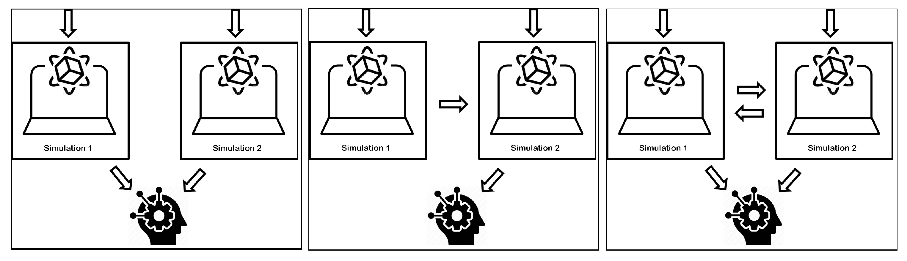
3.3. Synchronizing Simulations (The Time Dimension): The Operator ∘

Two simulations S 1 and S 2 to be composed that are executed in parallel and at different scales θ 1 and θ 2 have to be synchronized. The time step of a simulation is the smallest time interval between two simulation states ( t i t i 1 in u). A time step is atomic and cannot be divided. The middleware is inserted between these two simulations and will have a time step that is equal to Equation (5):
θ m i d d l e w a r e = min ( θ 1 , θ 2 )
In order to be able to execute its own time step t i , each simulation needs to know:
  • the demand (the portion of M o d that is being simulated at the moment t i ),
  • the route that these travelers will take from their origin to their destination.
Let S 1 and S 2 be two mobility simulations, with θ 1 > θ 2 , θ m i d d l e w a r e is then equal to θ 2 . The ∘ operator is implemented by the middleware by saving the consecutive u 2 output of S 2 until the next time step of S 1 is reached. At this point, the various saved outputs are composed and provided as input to the S 1 simulation. The output u 1 of S 1 is also retrieved, and provided to S 2 at its next time step.
The method to compose the different received u 2 and provided to S 1 depends on the three functions D emand , Assign , Move and will be described when describing the ⊕ operator (in Section 3.6).

3.4. Composing the Representations of Travelers: The • Operator

Consider two simulations S 1 and S 2 with two different representations ω 1 and ω 2 . The • operator transforms the two representations ω 1 and ω 2 to each other. We consider two bi-directional transformations: conversion of agents into flows (and vice versa) and (dis)aggregation of groups of agents.
To transform agents to flows, the middleware calculates a density and an average speed. We adopt the approach of [19] to do so:
  • For each vehicle, a function of its position x is defined: if the vehicle is present in x, then the function returns a positive constant, 0 otherwise.
  • Next, all previously defined functions are summed to create a new function. This new function thus returns a positive constant for each x position where a vehicle is present, 0 if no vehicle is present. This function is called D ( x ) .
  • Finally, if the cells of the model are spaced by Δ x , we obtain the density ρ k of traffic on the parts of the arc, necessary for the macroscopic model with the following function:
    ρ k = 1 Δ x k Δ x ( k + 1 ) Δ x D ( x ) d x
To transform flows to individual representation, it is necessary to create information for the individual agents. Indeed, a detailed simulation uses individual data that is not present in a simulation representing entities as flows. As a consequence, these data must be generated. To do so, we adopt the method of [19], who propose to create agents at positions determined by probabilities, following a Poisson process.
On the other side, to transform agents in groups of agents, we adopt the approach of [23], who propose to determine which agents to aggregate by defining distance functions between them and to aggregate the closest ones. However, two agents that are physically close cannot be aggregated if the probability that they will remain close in the future is low. We then use the similarity between itineraries instead of the similarity between positions.
The transformation of groups to individual agents follows the same procedure as the flows to agents transformation.

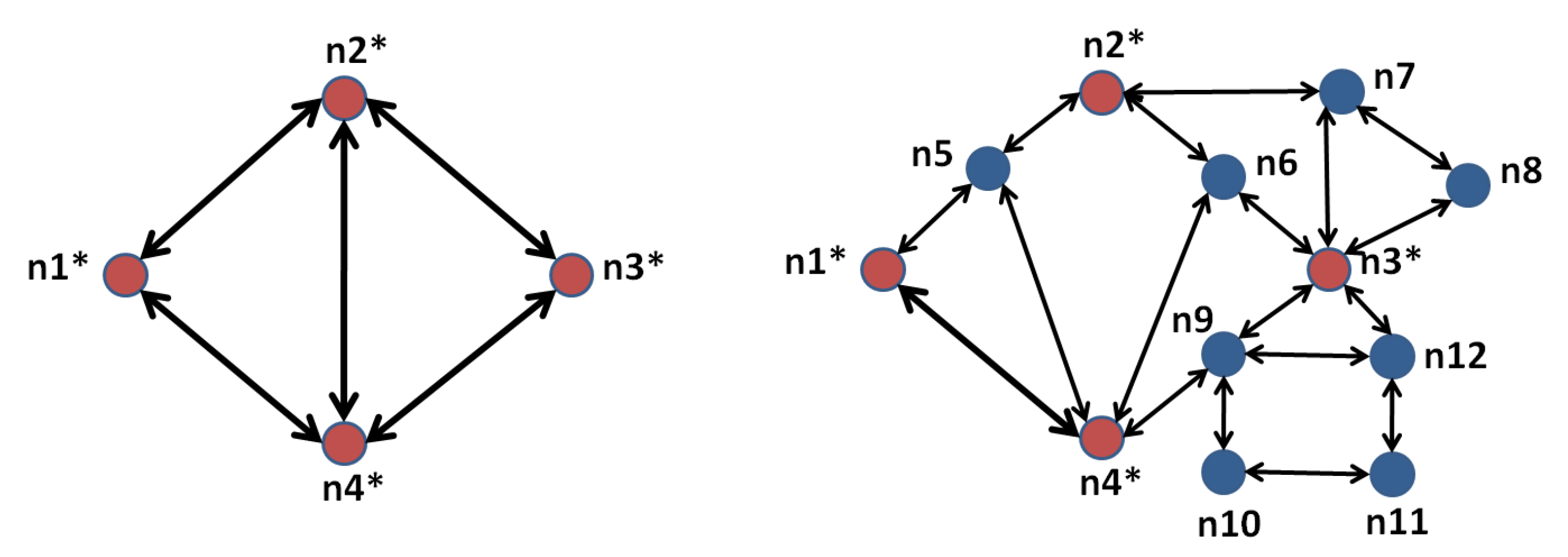
3.5. Composing Spatial Representations: The ⋄ Operator

Not all simulations represent the transportation network ( σ ) in the same way. The level of detail is not the same in a simulation of a few roads and in a simulation of an entire region. In some simulations where the represented area is wide, the transportation network is usually simplified. Some arcs of the network can be aggregated together or even deleted to optimize computation times, as explained in [37]. Figure 2 is an example of two representations of the same transportation network where the red nodes are present in both networks while the blue nodes are only found in the detailed representation.
Assumption 2
(Nodes co-existence). It is assumed that each node belonging to an aggregated representation of G exists also in the detailed representation. Moreover, for each arc present in the aggregated representation, there is at least one path in the detailed representation between the origin and the destination of this arc that does not pass through another node of the aggregated representation.
Therefore, we assume that, if there is a path from a node n1* to a node n4* in the aggregate representation without passing by a node n3* in the aggregated representation, then there is also a path in the detailed representation satisfying the same constraint.

3.6. Composing Processes: The ⊕ Operator
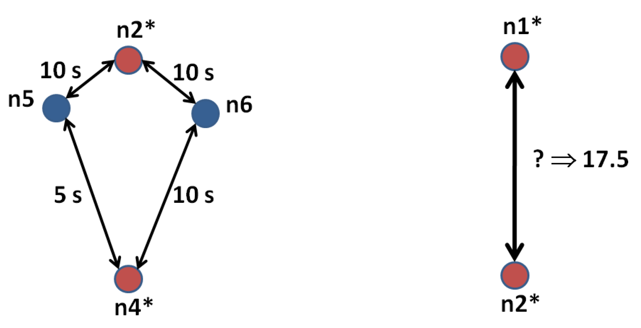
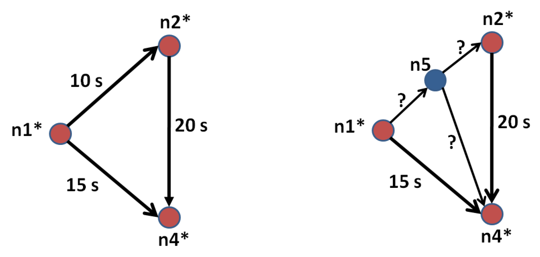
In this section, we detail the composition of the three functions of a simulation ( D emand , Assign , Move ). For clarity, the simulation noted S 1 in this section is always the one that corrects the considered function in the other simulation.

3.6.1. Composing Travel Times- M ove Functions

As a general rule, to correct the M ove function of a simulation S 2 by a simulation S 1 , the middleware modifies the travel times on the arcs traveled by S 2 by the average travel times observed on S 1 . This is done by changing the valuations of the relevant arcs in the graph G input of S 2 . This allows S 2 , whatever its scale, to apply its traffic model with the corrected travel times and speeds.
In the case of different ω (composed with the ∘ operator) between S 1 and S 2 , the middleware sends to S 2 a G graph with the observed average travel times.
In the case of different θ (composed with the ⋄ operator), the middleware executes as many time steps of S 1 until it covers a full time step of S 2 before executing S 2 with the right valuations of the G graph.
When we have a difference of spatial representation σ (composed with the • operator), the composition of the M ove functions is performed as follows. An arc in an aggregated spatial representation might represent one or several paths in the detailed spatial representation. To obtain the same travel times for travelers in each simulation, the average travel time of each arc in the aggregated representation has to be the same as the average travel time of its corresponding paths in the detailed representation.
Figure 3 shows the transition from the detailed network to the aggregated network. We compute the travel time of the aggregated link, as the average of the travel times of its corresponding paths. In the example of Figure 3, we obtain Equations (7) and (8):
T ( n 2 * , n 4 * ) a g g = 1 4 T ( n 2 * , n 5 ) d e t + T ( n 5 , n 4 * ) d e t + T ( n 2 * , n 6 ) d e t + T ( n 6 , n 4 * ) d e t
T ( n 2 * , n 4 * ) a g g = 17.5 s
Figure 4 shows the transition from aggregated to detailed representation. Once again, our goal is to obtain a travel time of the aggregated arcs equal to the average travel time of the corresponding paths in the detailed representation.
We then obtain the system of linear Equations (9)–(11):
T ( n 1 * , n 2 * ) a g g = T ( n 1 * , n 5 ) d e t + T ( n 5 , n 2 * ) d e t
T ( n 1 * , n 4 * ) a g g = 1 2 T ( n 1 * , n 5 ) d e t + T ( n 5 , n 4 * ) d e t + T ( n 1 * , n 4 * ) d e t r
T ( n 2 * , n 4 * ) a g g = T ( n 2 * , n 4 * ) d e t
There is an infinite number of solutions, such as:
T ( n 1 * , n 5 ) d e t = 5 s , T ( n 5 , n 2 * ) d e t = 5 s , T ( n 5 , n 4 * ) d e t = 10 s
T ( n 1 * , n 5 ) d e t = 6 s , T ( n 5 , n 2 * ) d e t = 4 s , T ( n 5 , n 4 * ) d e t = 11 s
Between all the available solutions, we choose the one offering the most homogeneous speeds (travel distance divided by the travel time).

3.6.2. Composing Demand: D emand Functions

Each simulation has its own M o d matrix. Whatever the scenario and scale considered, as soon as two simulations interact, they have to exchange travelers and inconsistencies may occur. This difference between the origin–destination matrices is taken into account in the two simulations (which are determined before execution) and the dynamic demand (which is calculated or obtained at each time step) must be taken into account when composing the D emand functions of S 1 and S 2 . In the general case, the middleware provides M o d 1 to S 2 at each time step, which it will consider instead of its own matrix.
In the case of a different σ with σ 1 more detailed than σ 2 , one must potentially find new origin and destination nodes for travelers in M o d 2 , since the nodes referenced in M o d 1 may not exist in M o d 2 . In this case, the middleware creates the travelers in the closest nodes. This case is not encountered if σ 2 is more detailed than σ 1 since all nodes of the detailed simulation exist in the aggregate simulation (cf. Assumption 2).

3.6.3. Composing Assignment: A ssign Functions

The correction of the assignment is achieved by the middleware through the valuation of the arcs in G, which makes the calculation of shorter path by S follow the result of the assignment made by S 1 (remember that the simulation noted S 1 is the one that corrects the considered function).
In the case of different ω (composed with the ∘ operator), the middleware has nothing particular to do, since the assignment concerns the valuation of arcs of G only.
In the case of different θ (composed with the ⋄ operator), the middleware will have to execute as many time steps of S 1 until it covers a full time step of S 2 before executing S 2 with the correct valuations of the G graph. This is necessary to execute S 2 with the right travel times.
In the case of a different σ (composed with the • operator), some paths existing in one representation do not exist in the other. The same procedure described for th Demand is applied here.

4. Inter-Dependency between Simulations

In the individual description of the ⊕ operator, we have considered individual functions compositions. However, in a multi-scale simulation, a first simulation usually corrects some function, while the second simulation corrects some other functions. In this case, in addition to the individual processes described earlier, some scheduling needs to be performed by the middleware. The processes described in this section are possible only if the considered simulations obey the following assumption.
Assumption 3
(Simulation Control). Some middleware features are applicable only to simulations that allow outside simulation control. Indeed, some corrections are only possible if we can momentarily stop a simulation, or restart a time step several times.
This assumption is necessary if the differences between the representations of the simulations can only be reconciled by controlling the simulations.
In Table 1, the second and third column present the functions that are considered valid for each simulation. The last column indicates if this type of inter-dependency needs to be treated in this section. Cases 1 and 2 are already covered by the previous section: There is no inter-dependency, and a simulation is fully dependent on the other.
The algorithms described in the next subsections materialize a natural scheduling of the different functions D emand , Assign and M ove in a four-step model. Indeed, we first define the demand, then we assign it and finally we simulate the travelers’ mobility. As a consequence, the simulation with the correct demand has to execute its time step first, then the simulation with the correct assignment, and finally the simulation with the right movements. The different cases in Table 1 are tackled in the following subsections, two by two.

4.1. Cases 3 and 8

In these cases, one simulation has a valid D emand function and the other has valid A ssign and M ove . Both simulations have to correct each others. This case can represent a situation where a local neighborhood simulation has a very detailed and validated modeling of the crowd dynamics, but its demand is coming from a wide-region simulation (e.g., in [38]). In this situation, the middleware needs to execute Algorithm 1 (called D-AM for Demand (first simulation)-Assign and Move (second simulation)).
Algorithm 1 D-AM algorithm.
Require: S d = ω d , σ d , θ d , P d ; S a m = ω a m , σ a m , θ a m , P a m ,
Ensure: S d a m = S d S a m
(1) ω d a m ω d ω a m
(2) σ d a m σ d σ a m
(3) θ d a m θ d θ a m
while ¬ E n d do
 (4) execute S d and save its demand M o d , S d in S d a m
 (5) execute S a m with the demand M o d , S d and save the resulting G S a m in S d a m
 (6) execute S d again with G S a m and save its demand M o d , S d in S d a m
end while
(7) Return S d a m
Instructions (1)–(3) allow for composing the scales of the involved simulations. To compose the processes, the middleware iteratively executes S d S a m S d , so that S d provides the right demand to S a m , which in turn provides the right valuations of the transportation graph (instructions (4)–(6)). Note that we use a simplified notation for the “execute” instruction: It actually means to execute as many time steps as necessary to cover a time step of the other simulation, as described in Section 3.3. The boolean E n d is set to true when the maximum time step is reached by one of the simulations.
In all the algorithms of this section, instruction (6) is the one that might be impossible to execute for all mobility simulations. Indeed, it implies re-executing the same time step of a simulation (a kind of rollback), but with different data. Since it is not always possible, we test in the experiments the case where only instructions (4) and (5) are executed (a unidirectional correction).

4.2. Cases 4 and 7

In these cases, one simulation has a valid A ssign function and the second simulation has valid D emand and M ove functions. This case can represent a situation where a simulation has its own valid demand (resulting from a recent survey for instance) and a valid traffic model (a properly calibrated car-following model for instance as in [39]), but the itineraries choice comes from a simulation-based traffic assignment (e.g., [40]).
In this situation, the middleware needs to execute Algorithm 2 (called A-DM for Assign-Demand and Move). Instructions (1)–(3) allow for composing the scales of the involved simulations. To compose the processes, the middleware iteratively executes S d m S a S d m , so that S d m provides the right demand to S a , which in turn provides the right valuations of the transportation graph (instructions (4)–(6)). Again, instruction (6) re-executes the same time step of S d m with a different graph ( G S a ).
Algorithm 2 A-DM algorithm.
Require: S a = ω a , σ a , θ a , P a ; S d m = ω d m , σ d m , θ d m , P d m ,
Ensure: S a d m = S a S d m
(1) ω a d m ω a ω d m
(2) σ a d m σ a σ d m
(3) θ a d m θ a θ d m
while ¬ E n d do
 (4) execute S d m and save its demand M o d , S d m in S a d m
 (5) execute S a with the demand M o d , S d m and save the resulting G S a in S a d m
 (6) execute S d m again with G S a and save its demand M o d , S d m in S a d m
end while
(7) Return S a d m

4.3. Cases 5 and 6

In these cases, one simulation has a valid M ove function and the second simulation has valid D emand and A ssign . In this situation, the middleware needs to execute Algorithm 3 (called M-DA for Move-Demand and Assign). Instructions (1)–(3) allow for composing the scales of the involved simulations. To compose the processes, the middleware iteratively executes S d a S m S d a , so that S d a provides the right demand to S m , which in turn provides the right valuations of the transportation graph (instructions (4), (5), and (6)). Again, instruction (6) re-executes the same time step of S d a with a different graph ( G S m ).
Algorithm 3 M-DA algorithm.
Require: S m = ω m , σ m , θ m , P m ; S d a = ω d a , σ d a , θ d a , P d a ,
Ensure: S m d a = S m S d a
(1) ω m d a ω m ω d a
(2) σ m d a σ m σ d a
(3) θ m d a θ m θ d a
while ¬ E n d do
 (4) execute S d a and save its demand M o d , S d a in S m d a
 (5) execute S m with the demand M o d , S d a and save the resulting G S m S m d a
 (6) execute S d a again with G S m and save its demand M o d , S d a in S m d a
end while
(7) Return S m d a

5. Experiments and Results
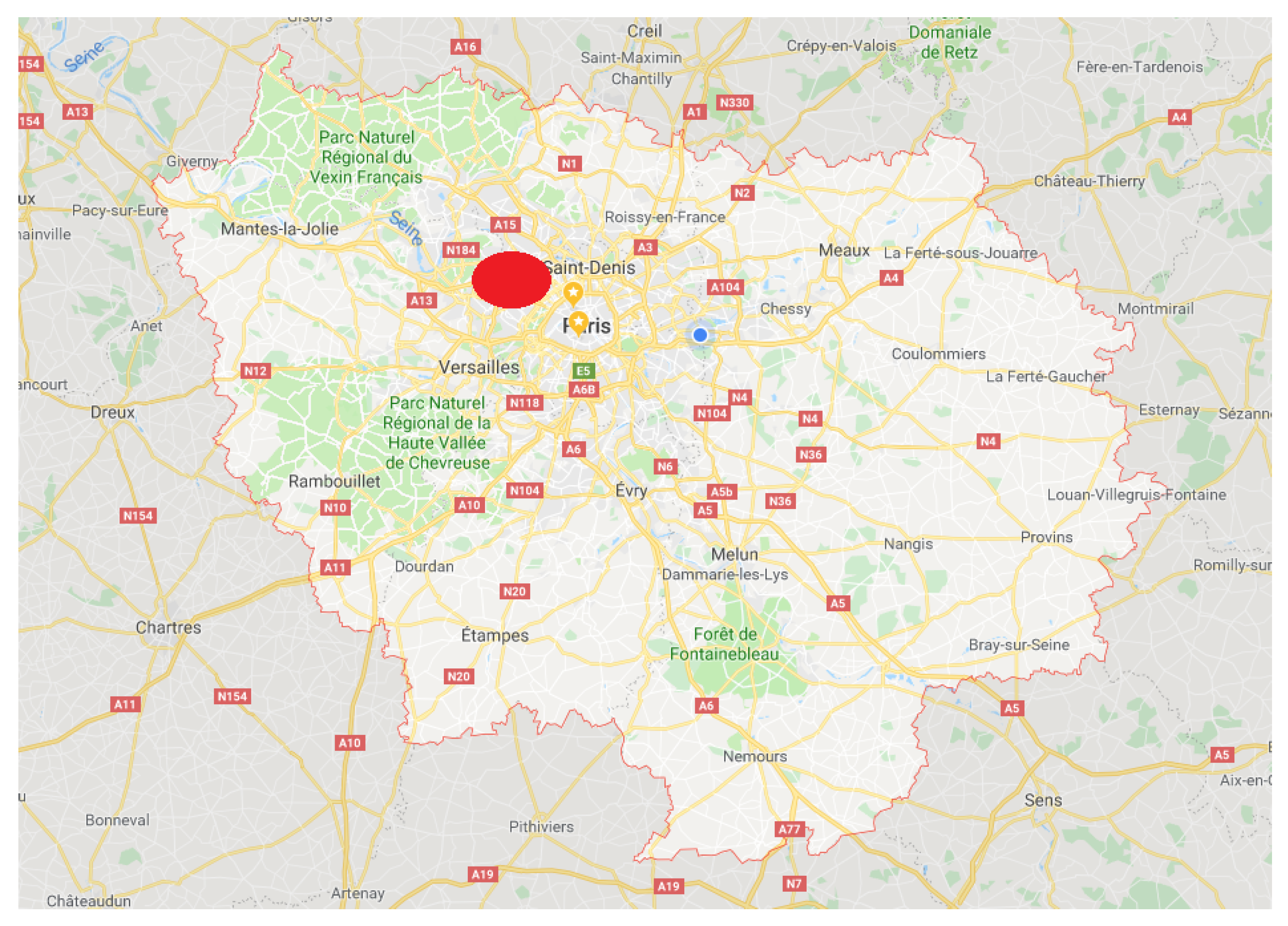
5.1. Case Study

This work is part of the MSM (Mobility Solution Modeling) project of the SystemX research institute. The MSM project is particularly interested in the issues of better knowledge and management of people’s mobility at the scale of a neighborhood. In this context, we imagine the tasks of a “neighborhood manager”, responsible for mobility management at the level of a given major neighborhood. In the project, we consider La Défense business district in the Paris region, with 180,000 employees and 20,000 inhabitants. The modes of transportation available in La Défense are multimodal, each managed by a different operator. The manager is interested in all the mobility taking place at La Défense (cf. Figure 5. To do so, it uses a multi-agent mobility simulation, which represents travelers individually, executes a few seconds time step and represents all the spatial details of the area.
However, as the neighborhood is not isolated from the world, mobility inside the neighborhood is highly dependent on travelers’ flows and transportation services upstream and downstream of the neighborhood. If an unforeseen event occurs at a location in the regional network (e.g., Châtelet—les Halles, a major multimodal hub in Paris), it is likely to have a great impact on the flows passing through or destined for La Défense. It is therefore necessary to have a knowledge of the dynamic status of the mobility at the region scale. However, it is neither necessary nor useful to represent regional flows as finely as the neighborhood (11 million travels/day in the Île de France region). Therefore, the regional simulation uses a mobility simulation where travelers are expressed in terms of flows, the network is represented in an aggregated way, and the time steps are several minutes long.

5.2. Middleware Implementation

We have implemented a middleware as a Java project, which implements all the model operators. The middleware interacts with interfaces, translating the input and output data from the involved simulations (cf. Figure 6). The use of these interfaces serves to keep the middleware independent from the languages and data types used by the simulations. When a new couple of simulations are considered, only the interfaces need to be implemented, and the middleware remains unchanged.
Parameters are defined for the middleware, in an XML file specifying, for each involved simulation:
  • The representation of travelers (flows, groups, or individual).
  • The length of a simulation time step in seconds.
  • The considered transportation network (following a defined XSD schema).
  • the functions that are considered valid for each simulation (Assign, Demand, and Move).

5.3. Setup

We use two simulations that we have developed in the context of the MSM project. The considered territories correspond to the use case described earlier (Île de France region and La Défense business district).
  • The first simulation is implemented in Java, and operates with traveler flows, on an aggregated network and with a time step of 10 min. It assigns travelers’ flows on the shortest route at Wardrop’s equilibrium using the transfer-and-equalize method [41]. The input of the simulation is:
    • The temporized origin–destination matrix on a region scale. These data are based on a National survey [42].
    • The aggregated network of the region (main streets only).
    Its output is the valuated graph every ten minutes.
  • The second simulation is implemented in Java, works with agents representing individual travelers, on a very detailed network and with a time step of 20 s. It assigns travelers using a K-shortest path algorithm [43]. This simulation uses a car-following model for travelers movements (Simplified Gipp Model from [44]). The inputs of this simulation are:
    • The temporized origin–destination matrix on the local scale. To obtain a matrix that is not too different from the regional matrix, we use the method described in [38] to infer a local matrix from a regional one. Then, we introduce some noise, by randomly multiplying the number of travelers in the matrix by a number in [ 10 , , 10 % ] .
    • The detailed network of the local area.
In the following, we assume that the regional simulation corrects the D emand and A ssign functions, while the local simulation corrects the M ove function. Therefore, the middleware applies the M-DA Algorithm (Algorithm 3).
Since the simulations and the middleware are all implemented in the same language, there is no need for an interface between them, and all interactions are performed using Java RMI (cf. Section 6 for a discussion on this aspect).
All the experiments have been performed using a unit under Linux Mint 17.2 Rafaela (kernel version 3.16.0-38-generic) with an Intel® Core processor CPU (Santa Clara, CA, USA) i5-7400 with 16 GB of memory.

5.4. Hypotheses

One of the objectives of the middleware is to harmonize the behaviors of simulations. More precisely, it allows for “correcting” the behavior of a simulation, based on another (valid) one. Four hypotheses are tested in the experiments.
Hypothesis 1
(Impact of the middleware). The use of the middleware allows for the behavioral convergence of two mobility simulations.
This is the first justification for using a middleware. We would expect that the difference in travel times or speeds are limited when using the middleware.
Hypothesis 2
(Impact of the difference in simulations’ behavior). The use of the middleware is more positive when the simulations have a big behavioral difference.
We would expect the middleware to have a bigger impact with simulations that have very different output (when used in isolation).
Hypothesis 3
(Impact of the scheduling). In case of inter-dependency, bidirectional corrections via the middleware provides better results than unidirectional corrections.
Not all simulation platforms allow for an external scheduling (by the middleware) allowing notably to execute several times (but with different inputs) the same time step (instructions (6) in Algorithms 1–3). If external scheduling is possible, we expect the middleware to have a higher impact. If this hypothesis is valid, it would be a strong argument for the simulation platforms to invest in the development of the right interfaces to allow an external scheduling.
Hypothesis 4
(Computational cost of the use of the middleware). The use of the middleware comes with a reasonable computational cost.
Interactive synchronized simulations come surely with a cost. However, we expect this cost to remain reasonable, i.e., not very far from max ( Θ S 1 , Θ S 2 ) , with Θ S 1 (resp. Θ S 2 ) the simulation time of S 1 (resp. S 2 ).

5.5. Scenarios

We simulate six different scenarios:
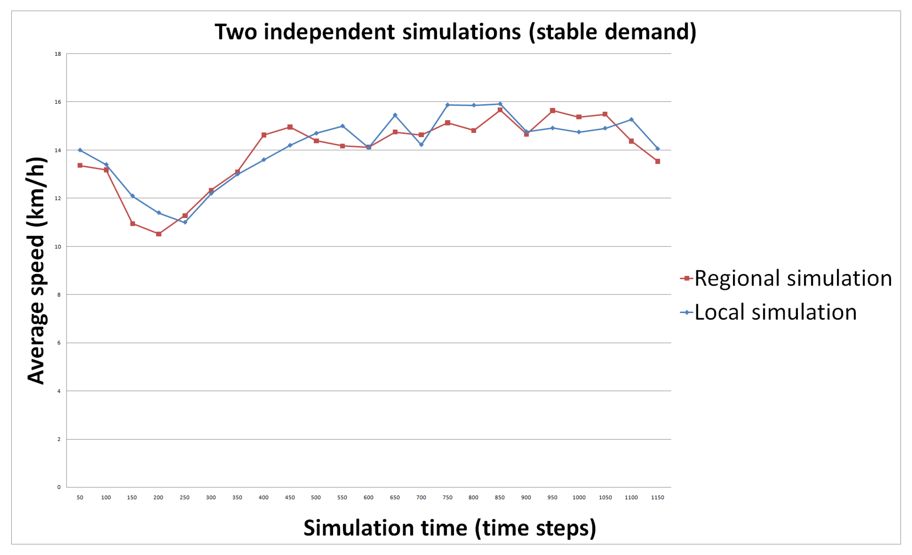
  • S1: we use each simulation independently. The demand is stable. To have a stable demand, we distribute the number of origin–destination equally over the available time slots in both regional and local origin–destination matrices.
  • S2: we use each simulation independently. The demand is variable (we use the original origin–destination matrices).
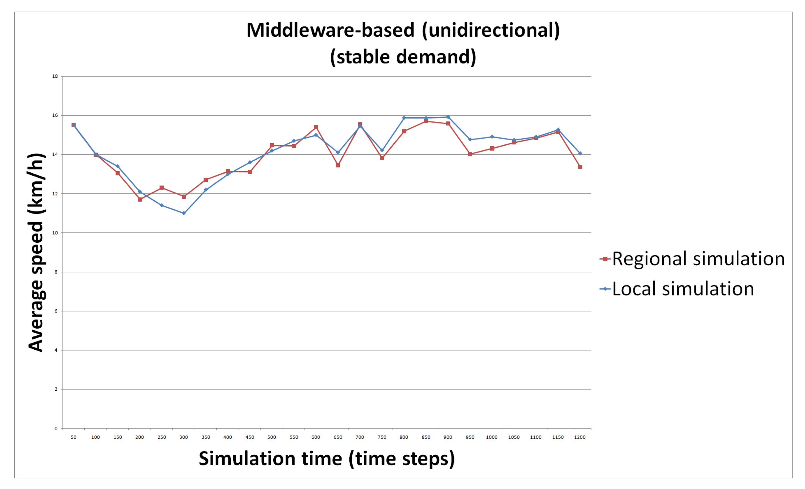
  • S3: we use the simulations interacting via the middleware. The interaction is unidirectional, meaning that a time step is not executed twice as defined in Section 4. Demand is stable.
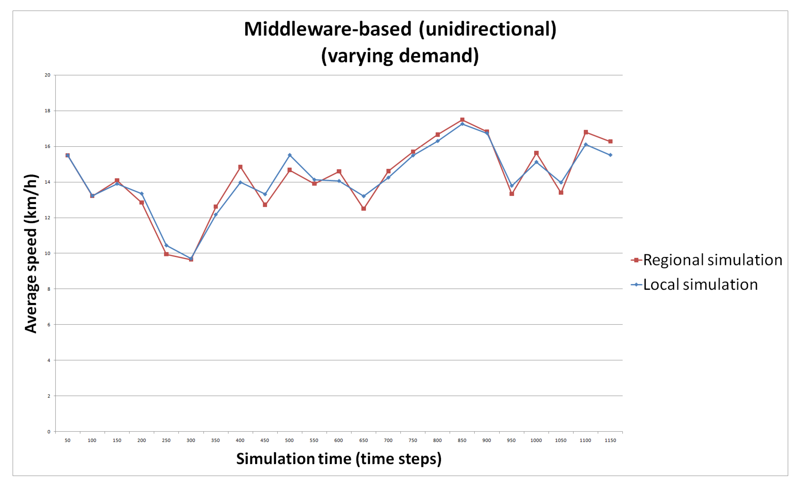
  • S4: we use the simulations interacting via the middleware. The interaction is unidirectional, meaning that a time step is not executed twice as defined in Section 4. Demand is variable.
  • S5: we use the simulations interacting via the middleware. The interaction is bidirectional, meaning that a time step is executed twice as defined in Section 4. Demand is stable.
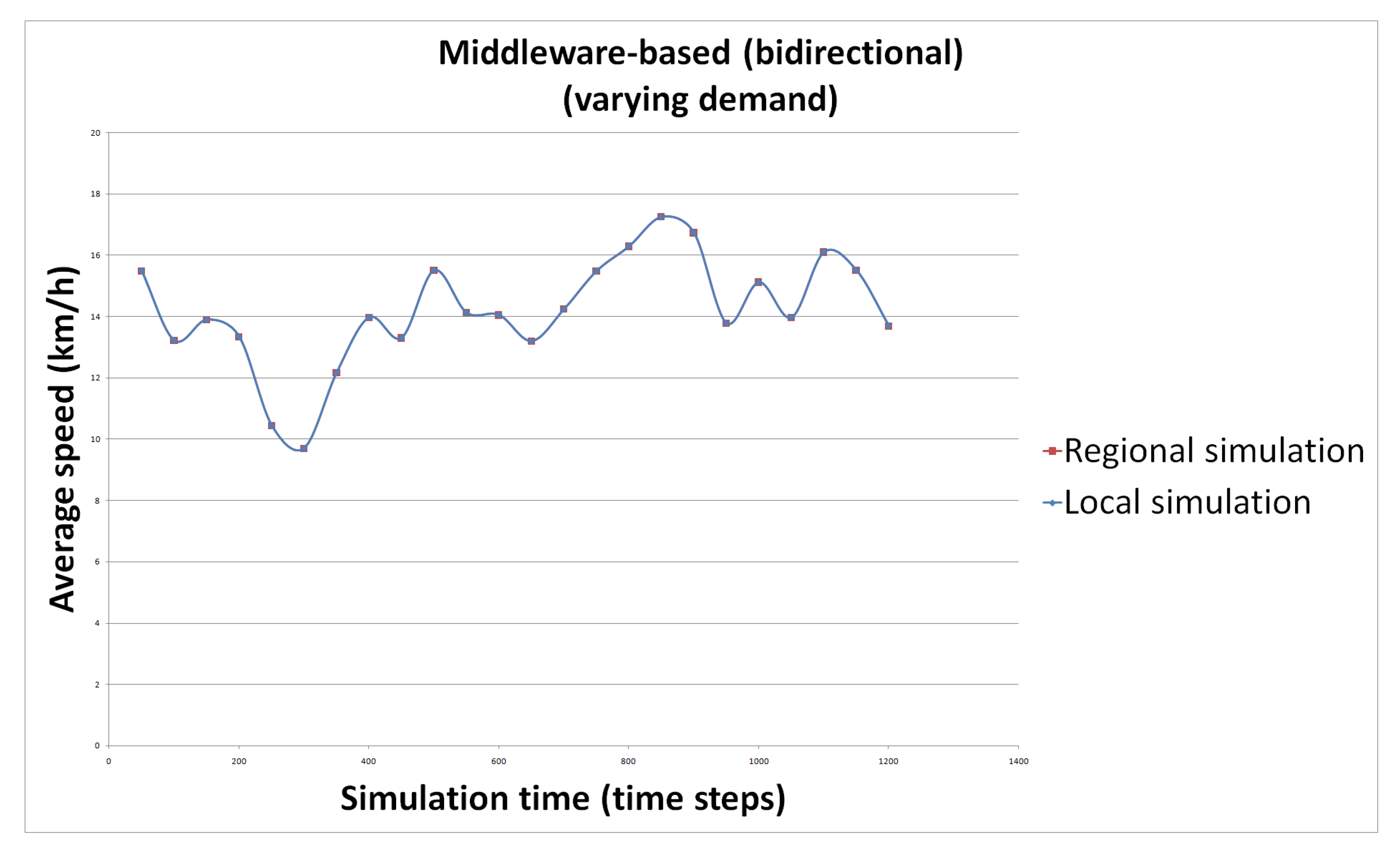
  • S6: we use the simulations interacting via the middleware. The interaction is bidirectional, meaning that a time step is executed twice as defined in Section 4. Demand is variable.
In every scenario, we compute the average speed observed in La Défense area (the local area). Indeed, since the local area is represented in both simulations, the impact of the middleware use is visible in this area. As we can observe in the input definition, the only source of randomness in our inputs concerns the temporized origin–destination matrix. To verify its impact, every set of scenarios is executed 10 times, with a different temporized origin–destination matrix. We observe a standard deviation of less than 0.2 km/h between the different executions of the same scenario. The results below report the average observed values.
The executed simulations represent 6 h and 40 min of travels. This corresponds to 1200 time steps of the local simulation and to 40 time steps of the regional simulation. In addition, 20,000 travelers are simulated in the local area during all the simulation.

5.6. Results

In Figure 7, Figure 8, Figure 9, Figure 10, Figure 11 and Figure 12, the x-axis represents the time steps of the local simulation, while the y-axis represents the observed average speeds.

5.6.1. Hypothesis 1

To verify this hypothesis (the use of the middleware allows for the behavioral convergence of two mobility simulations), we compare the scenario 1 (Figure 7) on the one side (average speeds for individual simulations) and scenarios 3 and 5 (average speeds for composed simulations) on the other side (Figure 9 and Figure 11). We note that the middleware succeeds in limiting (S3) and even eliminating (S5) the incoherence between the two simulations. The standard deviation of average speeds between the regional simulation and the local simulation is of 0.63 km/h in S1, 0.46 km/h in S3, and 0 km/h in S5. The difference may look small, but recall that the origin–destinations of the two simulations are quite similar ( ± 10 % ). Hypothesis 1 is then valid.

5.6.2. Hypothesis 2

To verify this hypothesis (the use of the middleware is more positive when the simulations have big behavioral difference), we compare the scenario 2 (Figure 8) on the one side (average speeds for individual simulations, with varying demand) and scenarios 4 and 6 (average speeds for composed simulations, with varying speeds) on the other side (Figure 10 and Figure 12). We note that the corrections of the middleware succeeds in limiting (S3) and even eliminating (S5) the incoherence between the two simulations. The standard deviation of average speeds is 0.92 km/h in S2, 0.52 km/h in S4 and 0 km/h in S6. The marginal correction is then of 0.4 (S4 compared to S2) and 0.92 (S6 compared to S2), while it was 0.17 (S3 compared to S1) and 0.63 (S5 compared to S1) with stable demand. Even if not very big, the difference is clearly there. Hypothesis 2 is then valid.

5.6.3. Hypothesis 3

To verify this hypothesis (bidirectional corrections via the middleware provides better results than unidirectional corrections), we compare the scenarios 3 and 5 on the one side (middleware without scheduling, cf. Figure 9 and Figure 11) and scenarios 4 and 6 on the other side (middleware wit scheduling, cf. Figure 10 and Figure 12). The standard deviations between average speeds is zero with the scheduling, while it is positive without it. Hypothesis 3 is valid.

5.6.4. Hypothesis 4

To verify this Hypothesis (the use of the middleware comes with a reasonable computational cost), we refer to Table 2 providing the computational times for the different scenarios. The use of the middleware with unidirectional correction provides reasonable increase in computational times compared to the regional simulation (which is the longest simulation between the two): 55 % (S3 compared to S1) and 65 % (S4 compared to S2). However, the use of the middleware with bidirectional correction results in a big increase in the computational times: 301 % (S5 compared to S1) and 369 % (S6 compared to S2) increase. The difference is big, and Hypothesis 4 is then not valid. Bidirectional correction has clear benefits, but it should be used when there are no tight constraints on execution times.

6. Conclusions

In the domain of software engineering, a lot of effort has been put for decades on applications’ interoperability. Now, several W3C standards, and industrial de facto standards, exist for applications deployed as web services (e.g., WS-* and Restful Web services) and on network representation (e.g., Openstreetmap). On the other side, in the domain of mobility simulations, the efforts on reusability of applications have mainly taken the form of open source deployment of simulations (e.g., SUMO [45], Matsim [46], etc.).
However, from a multi-scale simulation perspective, the designer of the middleware does not need to deeply master the implementation of the simulations; it only needs to use them as a service. It would therefore be very relevant to deploy mobility simulations as Web services, allowing for executing them, and to interact with them at a time step tempo. This effort is really worth it, since it would greatly simplify the design and implementation of new multi-scale simulations, with our middleware-based approach. In addition, this collective effort towards standard descriptions and use a service of simulations would greatly simplify the implementation of the interfaces described in Figure 6.
There is virtually an infinity of possible scenarios for mobility simulations. When facing a complex mobility scenario, involving several representation details (either spatial details, temporal details or details concerning the entities), the designer is often tempted to create a new simulation platform, fitting to his exact needs. However, tens of simulation platforms already exist, either as a research product or an industrial product. In many cases, there is no need to create a new simulation, and coupling existing simulations could be sufficient. If there is a general recommendation in this paper, it would be to consider carefully the creation of a new mobility simulation, and to verify if a composition of existing platforms fits the requirements of the scenario at hand.
For these cases, we propose a middleware model allowing for gluing existing mobility simulations working on different scales. Many of the presented methods in this paper are adaptations of existing methods in the literature. The results on a case study show that the use of the middleware limits, and can eliminate the incoherence between two simulations. However, having a perfect composition of the simulations with the middleware, including bidirectional correction, comes with a high computational cost. Depending on the requirements in terms of execution times, the designer might choose to use bidirectional or unidirectional corrections.
Our future work implies a great additional development effort: we will perform a systematic review of the existing mobility simulation platforms, create specific interfaces to interact with them (when possible), and use the middleware to assess the impact of the middleware on public mobility platforms and the relative easiness of coupling them with a middleware.

Author Contributions

Conceptualization, X.B. and M.Z.; methodology, M.Z.; software, X.B.; validation, X.B.; formal analysis, M.Z.; investigation, X.B.; resources, G.S. and F.L.; data curation, X.B.; writing—original draft preparation, X.B. and M.Z.; visualization, X.B.; supervision, M.Z., G.S., and F.L.; project administration, G.S. All authors have read and agreed to the published version of the manuscript.

Funding

This research received no external funding.

Data Availability Statement

Data available on request due to privacy restrictions.

Conflicts of Interest

The authors declare no conflict of interest.

References

  1. Nipa, T.J.; Kermanshachi, S.; Ramaji, I. Comparative analysis of strengths and limitations of infrastructure resilience measurement methods. In Proceedings of the 7th CSCE International Construction Specialty Conference (ICSC), Laval, QC, Canada, 12–15 June 2019; pp. 12–15. [Google Scholar]
  2. Ortega, F.A.; Pozo, M.A.; Puerto, J. On-line timetable rescheduling in a transit line. Transp. Sci. 2018, 52, 1106–1121. [Google Scholar] [CrossRef]
  3. Gan, H.; Ye, X. Will commute drivers switch to park-and-ride under the influence of multimodal traveler information? A stated preference investigation. Transp. Res. Part Traffic Psychol. Behav. 2018, 56, 354–361. [Google Scholar] [CrossRef]
  4. Bhattacharya, D.; Painho, M.; Mishra, S.; Gupta, A. Mobile traffic alert and tourist route guidance system design using geospatial data. Int. Arch. Photogramm. Remote Sens. Spat. Inf. Sci. 2017, 42, 11–18. [Google Scholar] [CrossRef] [Green Version]
  5. Nourinejad, M.; Roorda, M.J. Impact of hourly parking pricing on travel demand. Transp. Res. Part Policy Pract. 2017, 98, 28–45. [Google Scholar] [CrossRef]
  6. D’Ariano, A. Innovative decision support system for railway traffic control. IEEE Intell. Transp. Syst. Mag. 2009, 1, 8–16. [Google Scholar] [CrossRef]
  7. Toahchoodee, M.; Ray, I.; Anastasakis, K.; Georg, G.; Bordbar, B. Ensuring spatio-temporal access control for real-world applications. In Proceedings of the 14th ACM Symposium on Access Control Models and Technologies, Stresa, Italy, 3–5 June 2009; pp. 13–22. [Google Scholar]
  8. Zargayouna, M.; Othman, A.; Scemama, G.; Zeddini, B. Multiagent Simulation of Real-Time Passenger Information on Transit Networks. IEEE Intell. Transp. Syst. Mag. 2020, 12, 50–63. [Google Scholar] [CrossRef]
  9. Crociani, L.; Lämmel, G.; Vizzari, G. Multi-scale simulation for crowd management: A case study in an urban scenario. In Proceedings of the International Conference on Autonomous Agents and Multiagent Systems, Singapore, 9–13 May 2016; pp. 147–162. [Google Scholar]
  10. Zia, K.; Farrahi, K.; Riener, A.; Ferscha, A. An agent-based parallel geo-simulation of urban mobility during city-scale evacuation. Simulation 2013, 89, 1184–1214. [Google Scholar] [CrossRef]
  11. Mastio, M.; Zargayouna, M.; Scemama, G.; Rana, O. Distributed agent-based traffic simulations. IEEE Intell. Transp. Syst. Mag. 2018, 10, 145–156. [Google Scholar] [CrossRef]
  12. Anagnostopoulos, D. A methodological approach for model validation in faster than real-time simulation. Simul. Model. Pract. Theory 2002, 10, 121–139. [Google Scholar] [CrossRef]
  13. Hsu, C.; Lian, F.; Huang, C. A Systematic Spatiotemporal Modeling Framework for Characterizing Traffic Dynamics Using Hierarchical Gaussian Mixture Modeling and Entropy Analysis. IEEE Syst. J. 2014, 8, 1129–1138. [Google Scholar]
  14. Holmgren, J.; Ramstedt, L.; Davidsson, P.; Edwards, H.; Persson, J.A. Combining macro-level and agent-based modeling for improved freight transport analysis. Procedia Comput. Sci. 2014, 32, 380–387. [Google Scholar] [CrossRef] [Green Version]
  15. Fellendorf, M.; Vortisch, P. Microscopic traffic flow simulator VISSIM. In Fundamentals of Traffic Simulation; Springer: New York, NY, USA, 2010; pp. 63–93. [Google Scholar]
  16. Vliet, D.V. The Saturn Users Manual; Institute for Transportation Studies: Leeds, UK, 1998. [Google Scholar]
  17. Montero, L.; Codina, E.; Barceló, J.; Barceló, P. Combining macroscopic and microscopic approaches for transportation planning and design of road networks. In Proceedings of the 19 th ARRB Transport Research Conference, Sydney, Australia, 7–11 December 1998; pp. 93–108. [Google Scholar]
  18. Barceló, J.; Casas, J. Dynamic network simulation with AIMSUN. In Simulation Approaches in Transportation Analysis; Springer: New York, NY, USA, 2005; pp. 57–98. [Google Scholar]
  19. Sewall, J.; Wilkie, D.; Lin, M.C. Interactive hybrid simulation of large-scale traffic. ACM Trans. Graph. 2011, 30, 135. [Google Scholar] [CrossRef]
  20. Gaud, N.; Galland, S.; Gechter, F.; Hilaire, V.; Koukam, A. Holonic multilevel simulation of complex systems: Application to real-time pedestrians simulation in virtual urban environment. Simul. Model. Pract. Theory 2008, 16, 1659–1676. [Google Scholar] [CrossRef]
  21. Haman, I.T.; Kamla, V.C.; Galland, S.; Kamgang, J.C. Towards an multilevel agent-based model for traffic simulation. Procedia Comput. Sci. 2017, 109, 887–892. [Google Scholar] [CrossRef]
  22. Navarro, L.; Flacher, F.; Corruble, V. Dynamic level of detail for large scale agent-based urban simulations. In Proceedings of the 10th International Conference on Autonomous Agents and Multiagent Systems-Volume 2, Taipei, Taiwan, 2–6 May 2011; pp. 701–708. [Google Scholar]
  23. Navarro, L.; Corruble, V.; Flacher, F.; Zucker, J.D. A flexible approach to multi-level agent-based simulation with the mesoscopic representation. In Proceedings of the 2013 International Conference on Autonomous Agents and Multi-Agent Systems, Saint Paul, MN, USA, 6–10 May 2013; pp. 159–166. [Google Scholar]
  24. Biedermann, D.H.; Kielar, P.M.; Handel, O.; Borrmann, A. Towards TransiTUM: A generic framework for multiscale coupling of pedestrian simulation models based on transition zones. Transp. Res. Procedia 2014, 2, 495–500. [Google Scholar] [CrossRef] [Green Version]
  25. Joueiai, M.; Van Lint, H.; Hoogendoom, S.P. Multiscale traffic flow modeling in mixed networks. Transp. Res. Rec. 2014, 2421, 142–150. [Google Scholar] [CrossRef]
  26. Bishop, T.A.; Karne, R.K. A Survey of Middleware. In Proceedings of the ISCA 18th International Conference Computers and Their Applications, Honolulu, HI, USA, 26–28 March 2003; ISCA 2003. pp. 254–258. [Google Scholar]
  27. Klügl, F. A validation methodology for agent-based simulations. In Proceedings of the 2008 ACM Symposium on Applied Computing, Fortaleza, Brazil, 16–20 March 2008; pp. 39–43. [Google Scholar]
  28. Balci, O. Validation, verification, and testing techniques throughout the life cycle of a simulation study. Ann. Oper. Res. 1994, 53, 121–173. [Google Scholar] [CrossRef] [Green Version]
  29. Law, A.M. How to build valid and credible simulation models. In Proceedings of the Winter Simulation Conference, Orlando, FL, USA, 4–7 December 2005. [Google Scholar]
  30. Bayarri, M.; Berger, J.O.; Molina, G.; Rouphail, N.M.; Sacks, J. Assessing uncertainties in traffic simulation: A key component in model calibration and validation. Transp. Res. Rec. 2004, 1876, 32–40. [Google Scholar] [CrossRef] [Green Version]
  31. Ni, D. Multiscale modeling of traffic flow. Math. Aeterna 2011, 1, 27–54. [Google Scholar]
  32. Bourrel, E.; Lesort, J.B. Mixing microscopic and macroscopic representations of traffic flow: Hybrid model based on Lighthill–Whitham–Richards theory. Transp. Res. Rec. 2003, 1852, 193–200. [Google Scholar] [CrossRef]
  33. Gröger, G.; Kolbe, T.H.; Nagel, C.; Häfele, K.H. OGC City Geography Markup Language (CityGML) Encoding Standard; Technical Report; Open Geospatial Consortium: Wayland, MA, USA, 2012. [Google Scholar]
  34. Beil, C.; Kolbe, T.H. CityGML and the streets of New York-A proposal for detailed street space modelling. In Proceedings of the 12th International 3D GeoInfo Conference 2017, Melbourne, Australia, 26–27 October 2017; pp. 9–16. [Google Scholar]
  35. Lok, L.; Brent, R. Automatic generation of cellular reaction networks with Moleculizer 1.0. Nat. Biotechnol. 2005, 23, 131–136. [Google Scholar] [CrossRef] [PubMed]
  36. Szeto, W.; Wong, S. Dynamic traffic assignment: Model classifications and recent advances in travel choice principles. Cent. Eur. J. Eng. 2012, 2, 1–18. [Google Scholar] [CrossRef] [Green Version]
  37. Connors, R.D.; Watling, D.P. Assessing the demand vulnerability of equilibrium traffic networks via network aggregation. Netw. Spat. Econ. 2015, 15, 367–395. [Google Scholar] [CrossRef] [Green Version]
  38. Ksontini, F.; Zargayouna, M.; Scemama, G.; Leroy, B. Building a Realistic Data Environment for Multiagent Mobility Simulation. In Agent and Multi-Agent Systems: Technologies and Applications; Springer: New York, NY, USA, 2016; pp. 57–67. [Google Scholar]
  39. Raju, N.; Arkatkar, S.; Joshi, G. Evaluating performance of selected vehicle following models using trajectory data under mixed traffic conditions. J. Intell. Transp. Syst. 2019, 24, 617–634. [Google Scholar] [CrossRef]
  40. Szeto, W.Y. Dynamic modeling for intelligent transportation system applications. J. Intell. Transp. Syst. 2014, 18, 323–326. [Google Scholar] [CrossRef] [Green Version]
  41. Leurent, F. The theory and practice of a dual criteria assignment model with a continuously distributed value-of-time. In Proceedings of the Transportation and Traffic Theory Proceedings of the ISTTT Conference, Lyon, France, 24–26 July 1996; pp. 455–477. [Google Scholar]
  42. INSEE. Enquête Globale Transport. 2010. Available online: http://www.omnil.fr/IMG/pdf/-4.pdf (accessed on 19 January 2021).
  43. Eppstein, D. Finding the k shortest paths. SIAM J. Comput. 1998, 28, 652–673. [Google Scholar] [CrossRef] [Green Version]
  44. Treiber, M.; Kesting, A. Traffic flow dynamics. In Traffic Flow Dynamics: Data, Models and Simulation; Springer: Berlin/Heidelberg, Germany, 2013. [Google Scholar]
  45. Behrisch, M.; Bieker, L.; Erdmann, J.; Krajzewicz, D. SUMO- Simulation of Urban MObility—An Overview. In Proceedings of the Third International Conference on Advances in System Simulation, Barcelona, Spain, 23–28 October 2011; pp. 55–60. [Google Scholar]
  46. Maciejewski, M.; Nagel, K. Towards Multi-agent Simulation of the Dynamic Vehicle Routing Problem in MATSim. In Proceedings of the 9th International Conference on Parallel Processing and Applied Mathematics, Naleczow, Poland, 9–12 September 2012; pp. 551–560. [Google Scholar]
Figure 1. Simulations orchestrations (independent (left), sequential (middle), and parallel (right)).
Futureinternet 13 00022 g001
Figure 2. Different representations of the same area: Aggregated (left) and disaggregated (right).
Futureinternet 13 00022 g002
Figure 3. From travel times in the detailed representation (left) to the travel times in the aggregated representation (right).
Futureinternet 13 00022 g003
Figure 4. Calculation of the travel time of an arc of the detailed representation (right) from the aggregated representation (left).
Futureinternet 13 00022 g004
Figure 5. Use case study area (La Défense is located inside the red ellipse).
Futureinternet 13 00022 g005
Figure 6. Middleware implementation.
Futureinternet 13 00022 g006
Figure 7. Average speeds for Scenario S1.
Futureinternet 13 00022 g007
Figure 8. Average speeds for Scenario S2.
Futureinternet 13 00022 g008
Figure 9. Average speeds for Scenario S3.
Futureinternet 13 00022 g009
Figure 10. Average speeds for Scenario S4.
Futureinternet 13 00022 g010
Figure 11. Average speeds for Scenario S5.
Futureinternet 13 00022 g011
Figure 12. Average speeds for Scenario S6.
Futureinternet 13 00022 g012
Table 1. The different types of inter-dependency between multi-scale simulations.
# S 1 ’s Valid Function (s) S 2 ’s Valid Function (s)Inter-Dependency?
1Demand, Assign, Move-×
2-Demand, Assign, Move×
3DemandAssign, Move
4AssignDemand, Move
5MoveDemand, Assign
6Demand, AssignMove
7Demand, MoveAssign
8Assign, MoveDemand
Table 2. Execution times (in seconds) of the different scenarios in seconds.
ScenarioRegional SimulationLocal SimulationComposition
111003200-
215323840-
3--4945
4--6340
5--12,840
6--18,017
Publisher’s Note: MDPI stays neutral with regard to jurisdictional claims in published maps and institutional affiliations.

