An Extended Car-Following Model Considering Generalized Preceding Vehicles in V2X Environment

Abstract

Vehicle-to-everything (V2X) technology will significantly enhance the information perception ability of drivers and assist them in optimizing car-following behavior. Utilizing V2X technology, drivers could obtain motion state information of the front vehicle, non-neighboring front vehicle, and front vehicles in the adjacent lanes (these vehicles are collectively referred to as generalized preceding vehicles in this research). However, understanding of the impact exerted by the above information on car-following behavior and traffic flow is limited. In this paper, a car-following model considering the average velocity of generalized preceding vehicles (GPV) is proposed to explore the impact and then calibrated with the next generation simulation (NGSIM) data utilizing the genetic algorithm. The neutral stability condition of the model is derived via linear stability analysis. Numerical simulation on the starting, braking and disturbance propagation process is implemented to further study features of the established model and traffic flow stability. Research results suggest that the fitting accuracy of the GPV model is 40.497% higher than the full velocity difference (FVD) model. Good agreement between the theoretical analysis and the numerical simulation reveals that motion state information of GPV can stabilize traffic flow of following vehicles and thus alleviate traffic congestion.

1. Introduction

With the development of urbanization and motorization, the number of vehicles continues to grow, and congestion has become one of the main problems existing in cities around the world. Due to the limitation of urban space, previous methods of reducing traffic jams, such as building more infrastructure, have been producing very little effect. Regarded as an effective technological approach to improve transportation efficiency and alleviate traffic congestion, the intelligent transportation system (ITS) has received increasing attention. As one of the most important parts of ITS, V2X technology, which is the general term for communication and information technologies enabling vehicles to connect to everything [1,2], can significantly broaden the driver’s information perception range, enhance the driver’s information perception ability by enabling them to obtain the information about movement state of vehicles on the road. Compared with the ordinary traffic environment, driver’s car-following and other driving behavior, as well as traffic flow of following vehicles, will show different characteristics in the V2X environment [3,4,5]. The impact of the information mentioned above on car-following behavior and traffic flow was explored by scholars via constructing car-following models. Nagatani [6] proposed an extended car-following model and explored the impact of the non-neighboring front vehicle position information. Lenz et al. [7] and Ge et al. [8] respectively established a car-following model considering the headway of an arbitrary number of vehicles ahead in the current lane. Unlike Lenz believed that car-following behavior in the model was the result of multiple optimal velocity functions related to each headway, Ge believed that car-following behavior was the result of one optimal velocity function related to multiple headways. Chen et al. [9] further incorporated the desired following distance and explored the impact of this information by developing an improved car-following model. Li et al. [10] established an extended car-following model with consideration of the relative velocity of an arbitrary number of vehicles ahead. Hu et al. [11] further considered drivers’ reaction delay and extended the car-following model. Instead of drivers’ reaction delay, Guo et al. [12] further investigated velocity fluctuation feedback information. Peng et al. [13] presented an improved car-following model based on both headway and relative velocity information of an arbitrary number of preceding vehicles. Li et al. [14] proposed an extended car-following model to concurrently study headway, relative velocity and acceleration information of an arbitrary number of vehicles ahead in the current lane. Compared with the motion state information of an arbitrary number of vehicles ahead in the current lane, drivers incline to pay more attention to the motion state of vehicles that are in their view. For vehicles outside the field of view, drivers tend to focus on their overall motion state instead of individual motion state. Based on this, sun et al. [15] established an extended car-following model considering headway of the front vehicle and the average velocity of an arbitrary number of vehicles ahead in the current lane. Kuang et al. [16], Guo et al. [17] and Zhu et al. [18] presented modified car-following models to explore the information of average headway, average field velocity, the average desired velocity, respectively rather than than the average velocity. Soon afterward, Kuang et al. [19] built an extended car-following model with consideration of average velocity and average desired velocity in the meantime. Results of the above research revealed that providing motion state information of vehicles ahead in the current line to drivers could assist them to optimize car-following behavior and thus enhance the stability of traffic flow. However, urban roads are not all one-lane roads, and traffic flow on each lane of multi-lane roads is not independent of each other. Common driving experience also suggests that drivers will pay attention to motion state of vehicles ahead in the current and adjacent lanes at the same time. In recent years, a large number of research upon car-following behavior for different aims, such as traffic flow prediction [20], feedback control [21] or the safety analysis [22,23], and based on various idea, such as considering driver’ memory effect [24,25,26] or driver’s visual characteristics [27], communication delay [28], reaction delay [29], have been worked out. Among them, several efforts upon vehicle platoon control in V2X environment [30,31] or the influence of V2X technology on driving behavior [32,33] have been conducted. However, understanding about the impact exerted by motion state information, which is available for the drivers using V2X technology in ITS, of preceding vehicles including ones in the adjacent lanes on car-following behavior and traffic flow is still limited.

Motivated by the above contents, a concept called GPV is proposed to stand for the vehicles group consisted of the front vehicle, non-neighboring front vehicle, and neighboring front vehicles in the adjacent lanes (also known as left/right front vehicle), and average velocity is employed to represent motion state of GPV. Based on these, an extended car-following model is established in Section 2 and then calibrated with the NGSIM data set using the genetic algorithm in Section 3. The stability condition of the model is derived through linear stability analysis in Section 4, and the performance of our model is studied utilizing numerical simulation in Section 5. Based on these efforts, the impact of GPV motion state information on car-following behavior and traffic flow in the V2X environment is explored. Research results are discussed in Section 6, and the conclusion is given in Section 7.

2. Model

Car-following is the behavior, which is ubiquity in the traffic system, that driver manipulates his/her vehicle to follow the vehicles ahead. To study the characteristics of the car-following behavior and traffic flow, multi car-following models [34,35,36,37,38] were proposed based on various modeling ideas. Bando et al. [34] believe that drivers always attempt to keep a safe velocity depending on the headway between two successive vehicles when following the front vehicle. According to this, Bando proposed a car-following model called the optimal velocity (OV) model, and its motion equation is as follows:

$$\frac{d{v}_n(t)}{dt}=a\left[V\left(\Delta x_n\right)-v_n\left(t\right)\right]$$

(1)

where $a$ represents the sensitivity of the driver. $V\left(\Delta x_n\right)$ is the optimal velocity function, and $\Delta x_n=x_{n+1}(t)-x_n(t)$ denotes the headway of the two successive vehicles. $x_n(t)$ and $v_n(t)$ are, respectively, the position and velocity of the $n\hspace{0.17em}\mathrm{th}$ vehicle where $t$ represents time.

Helbing and Tilch [35] found that the OV model would work out excessive acceleration/deceleration during calibration of the optimal velocity function. To improve the OV model, Helbing established the generalized force (GF) model by introducing the negative velocity difference. Formulation of the GF model is as follows:

$$\frac{d{v}_n(t)}{dt}=a\left[V\left(\Delta x_n\right)-v_n\left(t\right)\right]+\lambda H\left[-\Delta v_n(t)\right]\Delta v_n(t)$$

(2)

where $a$ and $\lambda$ represent the sensitivity of the driver. $H$ is the Heaviside function and $\Delta v_n(t)=v_{j+1}-v_j$ is the velocity difference between the leading vehicle $j+1$ and the following vehicle $j$.

The GF model improved the OV model by solving the problem of excessive acceleration/deceleration. However, there are still some imperfections in the GF model. For instance, the following vehicle will not slow down when the headway is less than the minimum safety headway, and the preceding vehicle is going much faster. Motivated by these, Jiang et al. [36] constructed the full velocity difference (FVD) model by further considering the positive velocity difference. Its motion equation is as follows:

$$\frac{d{v}_n(t)}{dt}=a\left[V\left(\Delta x_n\right)-v_n\left(t\right)\right]+\lambda \Delta v_n(t)$$

(3)

Compared with the OV and CF models, the FVD model shows higher performance in simulating traffic flow and, especially, studying the stability of traffic flow.

However, the aforementioned models only reflect the interaction between the vehicle and its front vehicle. In a realistic traffic system, drivers not only focus on the vehicle ahead but also pay attention to multi preceding vehicles. Especially in a V2X environment, drivers can obtain massive information (for example, the velocity of an arbitrary number of vehicles ahead). Compared with an arbitrary number of vehicles ahead in the current lane, the driver would pay more attention to nearby vehicles, particularly the GPV, which are in the driver’s field of view. Among vehicles that are of GPV, the driver is primarily concerned with the vehicle in front of him/her to maintain a safe distance and avoid a collision. On this basis, the driver would also focus on GPV to optimize car-following behavior. Based on the above contents, an extended car-following model called the GPV model is proposed by introducing the average velocity of GPV, which can reflect the whole traffic situation on the segment [15]. The model’s dynamic equation is as follows:

$$\frac{d{v}_n(t)}{dt}=p\left\{a\left[V\left(\Delta x_n\right)-v_n\left(t\right)\right]+\lambda v_n\left(t\right)\right\}+\left(1-p\right)\left(\overline{v_n}-v_n\left(t\right)\right)$$

(4)

where $a$, $\lambda$ and $p$ respectively represent the sensitivity of driver about optimal velocity difference, velocity difference and the difference between GPV’s average velocity and self-vehicle velocity, and the drivers are assumed to be ideal and identical, which is expressed by a constant value of sensitivity in the GPV model. $\overline{v_n}$ is the average velocity of GPV and $\overline{v_n}=\left(v_{n+1}(t)+v_{n+2}(t)+v_l(t)+v_r(t)\right)/4$, where $v_{n+1}(t)$, $v_{n+2}(t)$, $v_l(t)$ and $v_r(t)$ are the velocity of the front vehicle, non-neighboring front vehicle, left and right front vehicles in the adjacent lanes.

In this research, the optimal velocity function calibrated with empirical data by Helbing [35] is employed:

$$V\left(\Delta x_n\right)=V_1+V_2\tanh \left[C_1\left(\Delta x_n-l_c\right)-C_2\right]$$

(5)

Parameters in Equation (5) are set, as shown in

Table 1. Parameters value in Equation (5).

Parameters	${\mathit{V}}_1$	${\mathit{V}}_2$	${\mathit{C}}_1$	${\mathit{C}}_2$	${\mathit{l}}_{\mathit{c}}$
	6.75	7.91	0.13	1.57	5

.

By substituting Equation (5) into Equation (4), Equation (4) can be rewritten as:

$$\frac{d{v}_n(t)}{dt}=p\left\{a\left[V_1+V_2\tanh \left[C_1\left(\Delta x_n-l_c\right)-C_2\right]-v_n\left(t\right)\right]+\lambda v_n\left(t\right)\right\}+\left(1-p\right)\left[{\overline{v}}_n-v_n\left(t\right)\right]$$

(6)

3. Parameter Calibration

NGSIM project initiated by the American Federal Highway Administration provides large-scale, high-precision vehicle trajectory data for the study of traffic flow theory, including the car-following model. The US101 data set of NGSIM is employed to celebrate the GPV model constructed in the previous section and then verify the celebration. To obtain suitable data for this specific work, selection of US101 data set need to be taken according to the following rules:

Rule 1: Lane number. The highway section where the US101 data set is collected is divided into 4 lanes, and 1 ramp numbered 1–5, as shown in Figure 1. Considering that lane 4 is next to ramp 5 and lane-changing behavior is frequent, vehicles in lane 4 and ramp 5 will not be regarded as object vehicle to eliminate interference on car-following behavior exerted by lane-changing behavior. Further considering that the front vehicles in the adjacent lanes are introduced into the GPV model, vehicles only in lane 2 can be regarded as an object vehicle.

Rule 2: Integrity of the vehicle group. GPV is comprehensively considered in our model, and thus the object vehicle for this research should have a complete GPV group. Based on this, the object vehicle for this research should have the front vehicle, non-neighboring front vehicle and left/right front vehicle to meet the integrity standard of the vehicle group.

Rule 3: Time headway between the object vehicle and its front vehicle. If time headway between the vehicle and its front vehicle exceeds 5 s [39], movement of the vehicle is no longer restricted by its front vehicle, and the vehicle will not be considered to be in a car-following state. Vehicles which are in the car-following state can be regarded as an object vehicle for our study.

Rule 4: Duration of car-following state. To ensure that the amount of data contained in each set of trajectory data are consistent and sufficient, the duration of the car-following behavior is set as 30 s considering characteristics of the US101 data set and its collection section.

According to rules 1–4, data filtering progress can be determined, as shown in Figure 2. Based on these, a selection of the US101 dataset is carried out, and 162 sets of trajectory data suitable for our research are obtained. Half of the datasets are randomly selected for calibrating model parameters, and the others are used to verify calibration results.

Calibration of parameters in the car-following model is a kind of optimum solution for nonlinear programming problems. In this work, the objective function is calculation error between actual data and model output, variables to be optimized are parameters in the model, and constraints are the physical boundaries of these parameters. The genetic algorithm is widely used and has shown high performance in dealing with this kind of problems [40,41]; parameters in the genetic algorithm used in this research are set as follows:

(a)

population size: 60;

(b)

crossover probability: 0.9;

(c)

mutation probability: 0.2;

(d)

iteration number: 500;

(e)

value range of parameters to be celebrated: $a\in \left[0,2\right]$, $\lambda \in \left[0,1\right]$, $p\in \left[0,1\right]$.

Utilizing MATLAB (Version 9.6) software, parameters in the GPV model is calibrated. The FVD model constructed in [36] is also calibrated for comparison and further exploration in the following sections. Calibration results are as shown in

Table 2. Calibration results of parameters in the generalized preceding vehicles (GPV) model and the full velocity difference (FVD) model.

Parameters	GPV Model	FVD Model
$a$	0.767	0.852
$\lambda$	0.301	0.389
$p$	0.769	—

.

To verify the calibration results of parameters in the GPV model and the FVD model, mean absolute error (MAE) and mean absolute relative error (MARE) are employed as the performance index. The equations of MAE and MARE are as follows:

$$MAE=\frac{1}{n}{\displaystyle \sum _{i=1}^n\left|y_i-y_i^m\right|}$$

(7)

$$MARE=\frac{1}{n}{\displaystyle \sum _{i=1}^n\left|\frac{y_i-y_i^m}{y_i}\right|}$$

(8)

where $y$ is the acceleration of the object vehicle. $y_i$ and $y_i^m$ represent, respectively, the $i\hspace{0.17em}\mathrm{th}$ measured value and $i\hspace{0.17em}\mathrm{th}$ calculated value with the model. The evaluation results of parameters calibration are as shown in

Table 3. Evaluation Results of the parameter calibrations.

Performance Index	GPV Model	FVD Model
MAE	1.4746	2.495
MARE	0.1712	3.2896

.

From Table 3, one can obtain that the calibration results are solid, and all performance indexes of the GPV model are superior to those of the FVD model. According to Table 3, we can obtain that the fitting accuracy of the GPV model to the data measured in the field is 40.497% higher than that of the FVD model. In order to further verify and evaluate the results of parameters calibration and explore the performance of the GPV model in fitting date measured in the field, we calculate acceleration using the GPV model and the FVD model with calibrated parameters and compare the calculation results with the 81 data sets which are randomly selected for verification in previous contents. Part of the comparison results is shown in Figure 3.

The comparison results reveal that the GPV model has higher fitting accuracy to data measured in the field than the FVD model. It is noteworthy that the fitting acceleration curve of the FVD model has bigger curvature in several places, and there is a certain delay in acceleration calculation results of the FVD model, especially in the deceleration phase. The causation of this phenomenon is that drivers adjust car-following behavior only according to the motion state of their front vehicle in the FVD model and cannot grasp the traffic situation further ahead, which will guide them to take measures in advance and thus reduce reaction delay. The above results suggest that GPV’s motion state, such as average velocity, plays an important role in improving the performance of the car-following model in fitting data measured in the field.

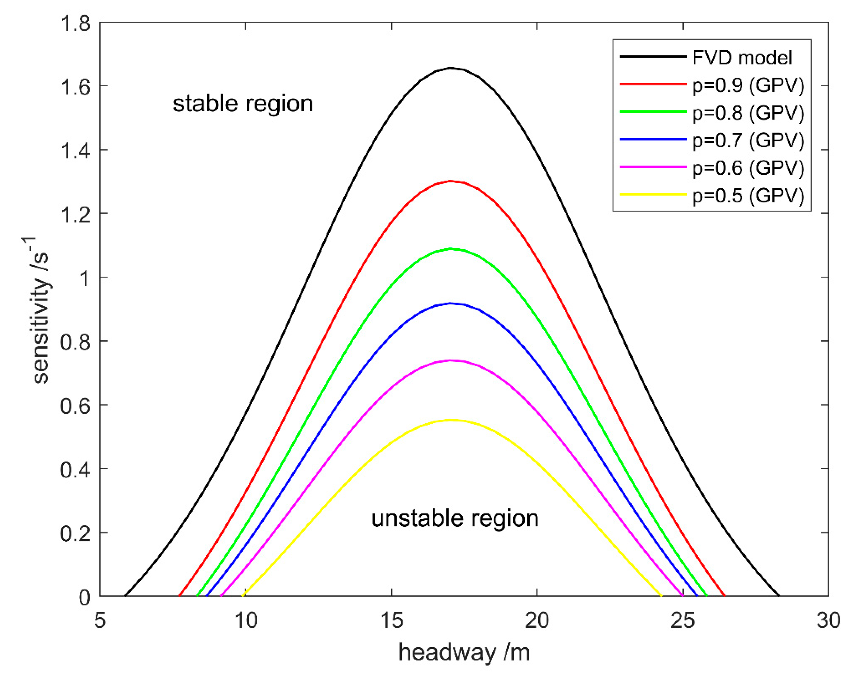
4. Stability Analysis

To explore the impact of average velocity information of GPV on traffic flow in the V2X environment, linear stability analysis is conducted based on the perturbation method [34,42,43]. Assuming that all three lanes in the system are in the same stable state, which means all vehicles maintain the same headway $h$ and velocity $V\left(h\right)$, at the initial moment, the position of the $n\hspace{0.17em}\mathrm{th}$ vehicle can be expressed as follows:

$$x_n^{(0)}(t)=hn+V\left(h\right)t$$

(9)

where $h=L/N$. $L$ is the length of the road and $N$ is the total number of vehicles on the road. $V\left(h\right)$ is the optimal velocity.

Suppose $y_n\left(t\right)$ to be a small deviation from the stable state solution $x_n^{(0)}(t)$

$$x_n(t)=x_n^{(0)}(t)+y_n\left(t\right)$$

(10)

Substituting Equations (9) and (10) into Equation (6) and linearizing the equation, one can obtain

$$\begin{array}{l}\frac{d^2{y}_n\left(t\right)}{d{t}^2}=p\left\{a\left[V’\left(h\right)\Delta y_n\left(t\right)-\frac{d{y}_n\left(t\right)}{dt}\right]+\lambda \frac{d\Delta y_n\left(t\right)}{dt}\right\}\\ +\left(1-p\right)\left[\frac{1}{4}\left(\frac{d{y}_{n+1}\left(t\right)}{dt}+\frac{d{y}_{n+2}\left(t\right)}{dt}+\frac{d{y}_l\left(t\right)}{dt}+\frac{d{y}_r\left(t\right)}{dt}\right)-\frac{d{y}_n\left(t\right)}{dt}\right]\end{array}$$

(11)

where $\Delta y_n\left(t\right)=y_{n+1}(t)-y_n(t)$ and $V’\left(h\right)={dV\left(\Delta x_n\right)/d\Delta x_n|}_{\Delta x_n=h}$. According to vehicles in all three lanes of the road are at the same stable state, one can obtain $\frac{d{y}_l\left(t\right)}{dt}=\frac{d{y}_r\left(t\right)}{dt}=\frac{d{y}_{n+1}\left(t\right)}{dt}$.

Substituting $y_n\left(t\right)=e^{ikn+zt}$ into Equation (11), one can obtain

$$z^2=p\left\{a\left[V’\left(h\right)\left(e^{ik}-1\right)-z\right]+\lambda z\left(e^{ik}-1\right)\right\}+\left(1-p\right)\left[\frac{1}{4}\left(3z{e}^{ik}+z{e}^{2ik}\right)-z\right]$$

(12)

By expanding $y_n\left(t\right)$, where $z=z_1\left(ik\right)+z_2{(ik)}^2+\cdots$, and inserting it into Equation (12), the first- and second-order terms of $ik$ can be obtained as follows:

$$z_1=V’\left(h\right)$$

(13)

$$z_2=\frac{2paV’\left(h\right)-4z_1{}^2+5(1-p)z_1+4p\lambda z_1}{4pa}$$

(14)

For long wavelength modes, the uniformly stable state traffic flow becomes unstable if $z_2<0$, while the uniformly stable state traffic flow remains stable if $z_2>0$. Therefore, the neutral stability condition is given as:

$$a=\frac{4V’\left(h\right)-5(1-p)-4p\lambda }{2p}$$

(15)

For small disturbances with long wavelengths, the uniform traffic flow is stable if

$$a>\frac{4V’\left(h\right)-5(1-p)-4p\lambda }{2p}$$

(16)

Based on Equation (15) and parameters calibrated in Section 3, the neutral stability curves of the GPV and FVD models in the headway-sensitivity space are as shown in Figure 4. From Figure 4, one can see that the headway-sensitivity phase space is divided into two regions by the neutral stability curves. The first is the stable region, which is above the corresponding neutral stability curve, and the second is the unstable region, which is below the corresponding neutral stability curve. In a stable region, traffic flow is stable, which means that small disturbances will be suppressed and, thus, traffic jams will not occur. In the unstable region, traffic flow is unstable, and density waves emerge. In this region, small disturbances cannot be suppressed effectively, and, on the contrary, it will gradually enlarge with propagation, which could lead to congestion eventually.

To explore the impact of the sensitivity parameter $p$ on the stability of traffic flow, the neutral stability curves of the GPV model with different $p$, as $p= 0.9,0.8,0.7,0.6,0.5$ respectively, are obtained when $\lambda =0.2$ as shown in Figure 5. From Figure 5, one can obtain that with the decrease p, the neutral stability curve gradually moves down, and the stable region keeps enlarging.

From Figure 4 and Figure 5, one can obtain that stable region of the GPV model is larger than that of the FVD model. This is because motion state of GPV considered in our model can assist driver with better grasping traffic condition ahead and taking measures in advance to maintain stable state as much as possible, and thus enhance the stability of traffic flow, which suggests that motion state such as average velocity of GPV plays an important role in enhancing the stability of traffic flow.

5. Numerical Simulation

To further verify analysis results in previous sections and study characterize features of the GPV model, numerical simulation on three typical traffic scenarios with comparison to the FVD model is carried out utilizing MATLAB (Version 9.6) software in this section. The three typical traffic scenarios, including the starting process, braking process as well as disturbance process, are constructed as shown in the following contents, and the motion state of vehicles in the scenarios are determined by the GPV model or the FVD model via numerical computation.

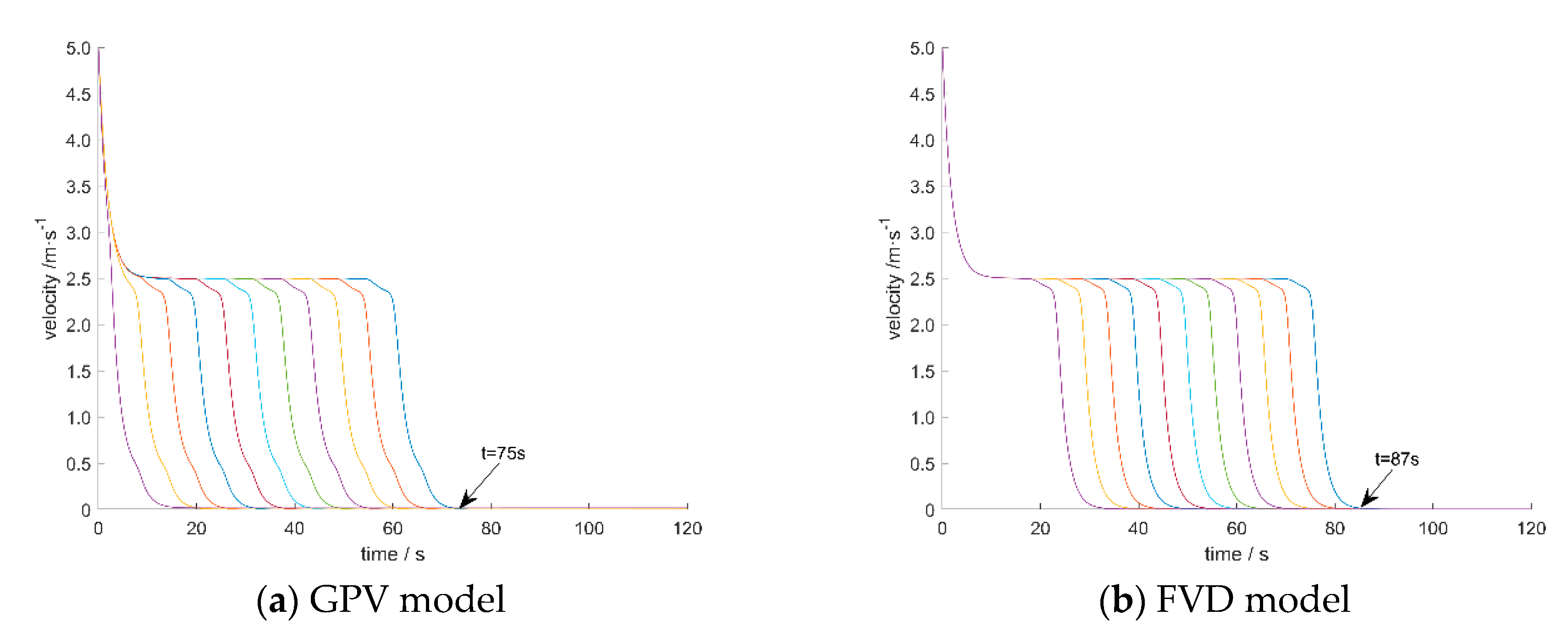
5.1. Simulation of Starting Process

To simulate the car-following behavior of vehicles in the starting process at the intersection when the traffic light turns from red to green in a realistic traffic system, the simulation scenario about vehicle starting process is set as the following: At an intersection with a traffic light, 10 identical vehicles stop and wait in every single of three lanes with the same headway of 10 m between any two consecutive vehicles, and all vehicles are about to start when the traffic light turns from red to green and move in the same direction. The vehicles in the middle of all three lanes are selected as object vehicles and marked as 1 to 10 according to the distance to the intersection from near to far. Considering that GPV is introduced in our model, the first object vehicle of the fleet is following its GPV in the scenario. At the beginning of the simulation, the traffic light turns green, and the vehicles start in sequence. The velocity limit of all object vehicles is set as 5 m/s, and the termination condition of this simulation is set as all object vehicles reach the velocity limit. The velocity and acceleration of all object vehicles are studied, as shown in Figure 6 and Figure 7.

Figure 6 illustrates the simulated velocity of the two models. As indicated in Figure 6a, it takes 19 s for all object vehicles to reach the preset velocity (5 m/s) in the simulation with the GPV model. By comparison, it takes 21 s to reach the same state with the FVD model, as shown in Figure 6b. (The lines with different color in Figure 6 as well as Figure 7, Figure 8 and Figure 9 respectively represents the object vehicles in the scenario.)

Figure 7 shows simulated acceleration with the two models. One can see that acceleration and accelerating time of the GPV model are less than those of the FVD model during the starting process. As shown in Figure 7a, the maximum acceleration is 1.6 m/s², and the acceleration process lasts 19 s with the GPV model. In contrast, the maximum acceleration is 1.8 m/s², and it cost an extra 3 s (total 21 s) to complete the acceleration process with the FVD model, as shown in Figure 7b.

5.2. Simulation of Braking Process

To simulate the car-following behavior of vehicles in the starting process at the intersection when the traffic light turns from red to green in a realistic traffic system, the simulation scenario about vehicle starting process is set as following: 10 identical vehicles in every single of three lanes are moving in the same direction with the same initial velocity 5 m/s and headway of 10 m between any two consecutive vehicles. The vehicles in the middle of all three lanes are selected as object vehicles and marked as 1 to 10 according to the distance to the intersection from near to far. Considering that GPV is introduced in our model, the first object vehicle of the fleet is following its GPV in the scenario. Moreover, regarding the comparability of simulation results, the scenario for simulation with the FVD model is set as the same. At the beginning of the simulation, the traffic light turns from green to red, and all vehicles brake in sequence. The termination condition of this simulation is set as all object vehicles have stopped. The velocity and the acceleration during the braking process of object vehicles are studied, as shown in Figure 8 and Figure 9.

Figure 8 depicts the simulated velocity of object vehicles with the GPV model and the FVD model, respectively, during the braking process. As shown in Figure 8a, it costs 16 s that the first vehicle of the fleet decelerates to 0 m/s, and all object vehicles stop at 75 s from the initial time in the simulation with the GPV model. By comparison, it takes 35 s that the first vehicle of the fleet decelerates to 0 m/s, and all object vehicles stop at 87 s from the beginning time in the simulation with the FVD model as shown in Figure 8b.

The simulated deceleration of object vehicles with the two models are as shown in Figure 9. In contrast with the FVD model, the deceleration of the GPV model is more rapid, and the response delay time is much shorter. As shown in Figure 9a, the first vehicle of the fleet reaches the maximum deceleration of 0.83 m/s² at 2.8 s, and the last vehicle of the fleet reaches the maximum deceleration of 0.5 m/s² at 61.1 s. By comparison, the first vehicle of the fleet reaches the maximum deceleration of 0.63 m/s² at 23.8 s, and the last vehicle of the fleet reaches the maximum deceleration of 0.63 m/s² at 76.1 s in this simulation with the FVD model as shown in Figure 9b.

From Figure 8 and Figure 9, one can see that there is a certain brake delay in the simulation with FVD and this result consistent with the results of data fitting in Section 3. Furthermore, it is worth noting that there are two deceleration fluctuations of each object vehicle during the braking process with the GPV model, while there is only one deceleration fluctuation with the FVD model. This phenomenon will be discussed in the following section.

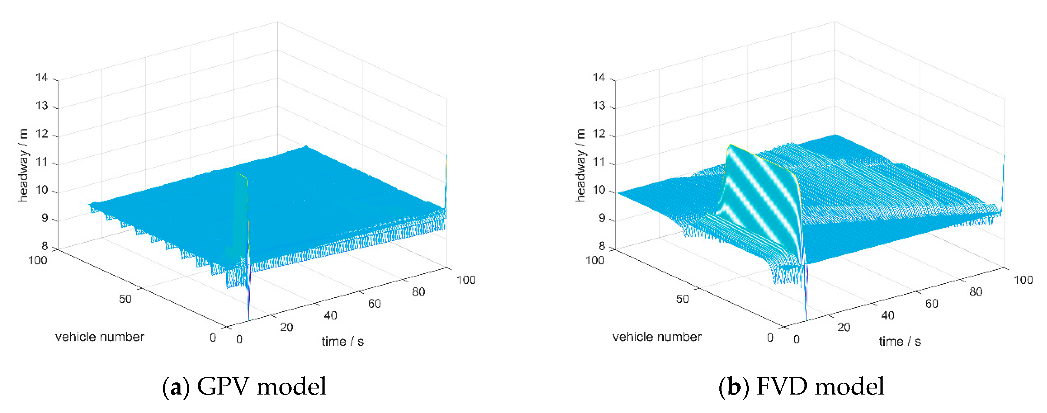
5.3. Simulation of Disturbance Propagation Process

The neutral stability curves of the GPV model and the FVD model are obtained in Section 4. According to the conclusion of the section, the headway–sensitivity phase diagram is divided into two regions. The region above neutral stability curves is the stable region, in which a small disturbance can be suppressed or absorbed. Simulation of the disturbance propagation process can represent the operation characteristics of traffic flow when an incident or accident occurs in a realistic traffic system and thus is employed to verify the above theoretical analysis results. The simulation scenario on propagation process of disturbance with the GPV model and the FVD model is set as following: 100 identical vehicles with a length of 5 m in each lane of three are moving towards the same direction on a 1500 m circular road with a constant velocity of 2 m/s and the same headway of 10 m. Then, a small disturbance of 1 m/s (half of the initial velocity) and 2 m (one-fifth of initial headway) is exerted on the vehicles, and the propagation process of this disturbance in the vehicle fleet is simulated as shown in Figure 10.

From Figure 10a, one can see that the same disturbance is rapidly suppressed to a small amplitude and finally absorbed with the GPV model. As shown in Figure 10b, this disturbance can be absorbed eventually with the FVD model. However, both the amplitude of the disturbance during the propagation process and the time for the disturbance to be absorbed are significantly greater than those of the GPV model, which has good agreement with the theoretical analysis results in Section 4.

6. Discussion

The information perception ability of the driver is significantly enhanced in the V2X environment. Utilizing V2X technology, drivers can obtain massive traffic information, and based on the information, adjust and optimize their car-following behavior. The impact of information about motion state of vehicle individuals such as headway, velocity and acceleration of preceding vehicles in the current lane on car-following behavior and traffic flow was studied in [6,7,8,9,10,11,12,13,14], and the impact of information about motion state of vehicles group including the average velocity of preceding vehicles in the current lane was explored in [15,16,17,18,19]. Although information about multi preceding vehicles, including left and the right front vehicle in the adjacent lanes, are available for drivers in the V2X environment, understanding about the influence of this information on car-following behavior and traffic flow is limited. Motived by this, a concept named GPV was proposed to represent the preceding vehicle group consisting of front vehicle, non-neighboring front vehicle and left/right front vehicle in the adjacent lanes, and average velocity was employed to represent the motion state of GPV. Based on these, an extended car-following model was established and then used to explore the impact exerted by motion state information of GPV on car-following behavior and traffic flow.

Research results reveal that motion state information of GPV can optimize driver’s car-following behavior and enhance the stability of traffic flow. In Section 3, the acceleration of object vehicles was calculated with the GPV model and the FVD model, respectively and compared with the verification data sets. The comparison (as shown in Figure 3) shows that the model established in this research with consideration of GPV motion state can better fit the data sets and reduce acceleration/deceleration delay existing in the FVD model. This illustrates that information about GPV motion state can enable drivers to grasp traffic situation ahead on the road instead of in the current lane and guide drivers to take measures in advance to decrease the response delay. The comparison results also reveal that taking GPV motion state account into the car-following model can make the model more in line with driving behavior characteristics, which is that drivers not only focus on the front vehicle but also pay attention to multi-preceding vehicles, including left/right front vehicles, and thus fit the measured data more accurately. In Section 4, the neutral stability condition of the GPV model was derived via linear stability analysis and then compared with that of the FVD model. The stability analysis results infer that considering the motion state of GPV can enhance the stability of traffic flow on a certain scale, and traffic flow will be more stable as more attention of drivers attached to the motion state of GPV. Explanation of these results are as follows: On one hand, information about the motion state of GPV can assist drivers with better understanding traffic situation ahead and guide them take measure earlier, which can effectively reduce reaction delay. On the other hand, with a better understanding of the traffic situation ahead, drivers can complete the maneuvering process with a relatively small acceleration/deceleration value to achieve a new stable driving state. Results in Section 3 and Section 4 suggest that GPV motion state information can effectively optimize driver’s car-following behavior and enhance traffic flow stability. Those results also confirm that it is necessary to take GPV into account into studying car-following behavior. To verify the above theoretical analysis results and to present the characteristics of the GPV model in an intuitive way, the numerical simulation based on three typical traffic scenarios with GPV and FDV model was conducted for contrastive analysis in Section 5. The results of numerical simulation agree well with the above analysis. Among the simulation results, one is noteworthy that there are two deceleration fluctuations during the braking process with the GPV model, and there is one fluctuation in the same scenario with the FVD model. This may be caused by drivers adopt larger deceleration values to maintain a safe distance and avoid a collision as the headway between the object vehicle and its front vehicle decreases, which in line with that, safety is the first primary interest for all drivers.

With these results, we believe that in the V2X environment, information of GPV motion state can assist drivers in optimizing car-following behavior and, thus, enhance the stability of traffic flow, which infer that traffic efficiency will be improved and energy consumption will be reduced with V2X technology in ITS. The above results also suggest that GPV should be taken into account in car-following research. Finally, it must be pointed out that we assumed all vehicles and their drivers are ideal and identical to eliminate the influence caused by the heterogeneity of the vehicles and their drivers, and we look forward to exploring this influence in our future research.

7. Conclusions

The impact of information about GPV motion state in V2X environment upon car-following behavior and traffic flow was studied by establishing an extended car-following model (called the GPV model) in this work. The fitting accuracy of the GPV model to the data measured in the field is 40.497% higher than that of the FVD model. Research results reveal that the motion state of GPV, which should be considered in research about car-following behavior, can assist drivers to optimize their car-following behavior and enhance the stability of traffic flow efficiently. These results confirm that the application of V2X technology in ITS will alleviate traffic jams, improve transportation efficiency, and thus reduce the energy consumption of the transportation system to a certain extent.

References

1. Seo, H.; Lee, K.-D.; Yasukawa, S.; Peng, Y.; Sartori, P. LTE evolution for vehicle-to-everything services. IEEE Commun. Mag. 2016, 54, 22–28. [Google Scholar] [CrossRef]
2. Storck, C.R.; Duarte-Figueiredo, F. A 5G V2X Ecosystem Providing Internet of Vehicles. Sensors 2019, 19, 550. [Google Scholar] [CrossRef] [PubMed] [Green Version]
3. Farah, H.; Koutsopoulos, H.N. Do cooperative systems make drivers’ car-following behavior safer? Transp. Res. Part C Emerg. Technol. 2014, 41, 61–72. [Google Scholar] [CrossRef]
4. Li, X.; Cui, J.; An, S.; Parsafard, M. Stop-and-go traffic analysis: Theoretical properties, environmental impacts and oscillation mitigation. Transp. Res. Part B Methodol. 2014, 70, 319–339. [Google Scholar] [CrossRef]
5. Jia, D.; Ngoduy, D. Enhanced cooperative car-following traffic model with the combination of V2V and V2I communication. Transp. Res. Part B Methodol. 2016, 90, 172–191. [Google Scholar] [CrossRef]
6. Nagatani, T. Stabilization and enhancement of traffic flow by the next-nearest-neighbor interaction. Phys. Rev. E 1999, 60, 6395–6401. [Google Scholar] [CrossRef] [Green Version]
7. Lenz, H.; Wagner, C.; Sollacher, R. Multi-anticipative car-following model. Eur. Phys. J. B 1999, 7, 331–335. [Google Scholar] [CrossRef]
8. Ge, H.X.; Shiqiang, D.; Dong, L.Y.; Xue, Y. Stabilization effect of traffic flow in an extended car-following model based on an intelligent transportation system application. Phys. Rev. E 2004, 70, 066134. [Google Scholar] [CrossRef]
9. Chen, J.; Liu, R.; Ngoduy, D.; Shi, Z. A new multi-anticipative car-following model with consideration of the desired following distance. Nonlinear Dyn. 2016, 85, 2705–2717. [Google Scholar] [CrossRef]
10. Li, Z.-P.; Liu, Y.-C. Analysis of stability and density waves of traffic flow model in an ITS environment. Eur. Phys. J. B 2006, 53, 367–374. [Google Scholar] [CrossRef]
11. Hu, Y.; Ma, T.; Chen, J. An extended multi-anticipative delay model of traffic flow. Commun. Nonlinear Sci. Numer. Simul. 2014, 19, 3128–3135. [Google Scholar] [CrossRef]
12. Guo, L.; Zhao, X.; Yu, S.; Li, X.; Shi, Z. An improved car-following model with multiple preceding cars’ velocity fluctuation feedback. Phys. A Stat. Mech. Appl. 2017, 471, 436–444. [Google Scholar] [CrossRef]
13. Peng, G.; Sun, D. A dynamical model of car-following with the consideration of the multiple information of preceding cars. Phys. Lett. A 2010, 374, 1694–1698. [Google Scholar] [CrossRef]
14. Li, Y.; Sun, D.; Liu, W.; Zhang, M.; Zhao, M.; Liao, X.; Tang, L. Erratum to: Modeling and simulation for microscopic traffic flow based on multiple headway, velocity and acceleration difference. Nonlinear Dyn. 2011, 66, 845. [Google Scholar] [CrossRef] [Green Version]
15. Sun, D.; Kang, Y.; Yang, S. A novel car following model considering average speed of preceding vehicles group. Phys. A Stat. Mech. Appl. 2015, 436, 103–109. [Google Scholar] [CrossRef]
16. Kuang, H.; Xu, Z.-P.; Li, X.-L.; Lo, S. An extended car-following model accounting for the average headway effect in intelligent transportation system. Phys. A Stat. Mech. Appl. 2017, 471, 778–787. [Google Scholar] [CrossRef]
17. Guo, Y.; Xue, Y.; Shi, Y.; Wei, F.-P.; Lü, L.-Z.; He, H.-D. Mean-field velocity difference model considering the average effect of multi-vehicle interaction. Commun. Nonlinear Sci. Numer. Simul. 2018, 59, 553–564. [Google Scholar] [CrossRef]
18. Wen-Xing, Z.; Li-Dong, Z. A new car-following model for autonomous vehicles flow with mean expected velocity field. Phys. A Stat. Mech. Appl. 2018, 492, 2154–2165. [Google Scholar] [CrossRef]
19. Kuang, H.; Wang, M.-T.; Lu, F.-H.; Bai, K.-Z.; Li, X.-L. An extended car-following model considering multi-anticipative average velocity effect under V2V environment. Phys. A Stat. Mech. Appl. 2019, 527, 121268. [Google Scholar] [CrossRef]
20. Xiao, X.; Duan, H.; Wen, J. A novel car-following inertia gray model and its application in forecasting short-term traffic flow. Appl. Math. Model. 2020, 87, 546–570. [Google Scholar] [CrossRef]
21. Jin, Y.; Meng, J. Dynamical analysis of an optimal velocity model with time-delayed feedback control. Commun. Nonlinear Sci. Numer. Simul. 2020, 90, 105333. [Google Scholar] [CrossRef]
22. Jian, M.; Shi, J. Analysis of impact of elderly drivers on traffic safety using ANN based car-following model. Saf. Sci. 2020, 122, 104536. [Google Scholar] [CrossRef]
23. Jiao, S.; Zhang, S.; Zhou, B.; Zhang, L.; Xue, L. Dynamic performance and safety analysis of car-following models considering collision sensitivity. Phys. A Stat. Mech. Appl. 2020, 564, 125504. [Google Scholar] [CrossRef]
24. Cao, B.-G. A car-following dynamic model with headway memory and evolution trend. Phys. A Stat. Mech. Appl. 2020, 539, 122903. [Google Scholar] [CrossRef]
25. Zhai, C.; Wu, W. A new continuum model with driver’s continuous sensory memory and preceding vehicle’s taillight. Commun. Theor. Phys. 2020, 72, 105004. [Google Scholar] [CrossRef]
26. Ma, G.; Ma, M.; Liang, S.; Wang, Y.; Guo, H. Nonlinear analysis of the car-following model considering headway changes with memory and backward looking effect. Phys. A Stat. Mech. Appl. 2021, 562, 125303. [Google Scholar] [CrossRef]
27. Mai, M.; Wang, L.; Prokop, G. Advancement of the car following model of Wiedemann on lower velocity ranges for urban traffic simulation. Transp. Res. Part F Traffic Psychol. Behav. 2019, 61, 30–37. [Google Scholar] [CrossRef]
28. Zhang, G.; Yin, L.; Pan, D.-B.; Zhang, Y.; Cui, B.-Y.; Jiang, S. Research on multiple vehicles’ continuous self-delayed velocities on traffic flow with vehicle-to-vehicle communication. Phys. A Stat. Mech. Appl. 2020, 541, 123704. [Google Scholar] [CrossRef]
29. Ma, L.; Qu, S. A sequence to sequence learning based car-following model for multi-step predictions considering reaction delay. Transp. Res. Part C Emerg. Technol. 2020, 120, 102785. [Google Scholar] [CrossRef]
30. Wang, P.; Di, B.; Zhang, H.; Bian, K.; Song, L. Platoon Cooperation in Cellular V2X Networks for 5G and Beyond. IEEE Trans. Wirel. Commun. 2019, 18, 3919–3932. [Google Scholar] [CrossRef]
31. Li, Y.; Chen, W.; Peeta, S.; Wang, Y. Platoon Control of Connected Multi-Vehicle Systems under V2X Communications: Design and Experiments. IEEE Trans. Intell. Transp. Syst. 2020, 21, 1891–1902. [Google Scholar] [CrossRef]
32. Sequeira, L.; Szefer, A.; Slome, J.; Mahmoodi, T. A Lane Merge Coordination Model for a V2X Scenario. In Proceedings of the 2019 European Conference on Networks and Communications (EuCNC); Institute of Electrical and Electronics Engineers (IEEE), Valencia, Spain, 18–21 June 2019; pp. 198–203. [Google Scholar]
33. Jia, B.; Yang, D.; Zhang, X.; Wu, Y.; Guo, Q. Car-following model considering the lane-changing prevention effect and its stability analysis. Eur. Phys. J. B 2020, 93, 1–9. [Google Scholar] [CrossRef]
34. Bando, M.; Hasebe, K.; Nakayama, A.; Shibata, A.; Sugiyama, Y. Dynamical model of traffic congestion and numerical simulation. Phys. Rev. E 1995, 51, 1035–1042. [Google Scholar] [CrossRef] [PubMed]
35. Helbing, D.; Tilch, B. Generalized force model of traffic dynamics. Phys. Rev. E 1998, 58, 133–138. [Google Scholar] [CrossRef] [Green Version]
36. Jiang, R.; Wu, Q.; Zhu, Z. Full velocity difference model for a car-following theory. Phys. Rev. E 2001, 64, 017101. [Google Scholar] [CrossRef] [Green Version]
37. Treiber, M.; Helbing, D. Memory effects in microscopic traffic models and wide scattering in flow-density data. Phys. Rev. E 2003, 68, 046119. [Google Scholar] [CrossRef] [Green Version]
38. Peng, Y.; Liu, S.; Yu, D.Z. An improved car-following model with consideration of multiple preceding and following vehicles in a driver’s view. Phys. A Stat. Mech. Appl. 2020, 538, 122967. [Google Scholar] [CrossRef]
39. Yang, X.; Zhang, N. An Improved Method of Determining Car-Following State. J. Transp. Syst. Eng. Inf. Technol. 2006, 14–17. [Google Scholar] [CrossRef]
40. Sangster, J.; Rakha, H.; Du, J. Application of Naturalistic Driving Data to Modeling of Driver Car-Following Behavior. Transp. Res. Rec. J. Transp. Res. Board 2013, 2390, 20–33. [Google Scholar] [CrossRef]
41. Zhu, M.; Wang, X.; Tarko, A.; Fang, S. Modeling car-following behavior on urban expressways in Shanghai: A naturalistic driving study. Transp. Res. Part C Emerg. Technol. 2018, 93, 425–445. [Google Scholar] [CrossRef] [Green Version]
42. Yu, L.; Shi, Z.; Zhou, B. Kink–antikink density wave of an extended car-following model in a cooperative driving system. Commun. Nonlinear Sci. Numer. Simul. 2008, 13, 2167–2176. [Google Scholar] [CrossRef]
43. Yao, Z.; Xu, T.; Jiang, Y.; Hu, R. Linear stability analysis of heterogeneous traffic flow considering degradations of connected automated vehicles and reaction time. Phys. A Stat. Mech. Appl. 2021, 561, 125218. [Google Scholar] [CrossRef]
Figure 1. Lane setting of US101 collection section.
Futureinternet 12 00216 g001
Figure 2. Data filtering progress of the US101 data set.
Futureinternet 12 00216 g002
Figure 3. Comparison of computational acceleration between the GPV model and the FVD model with the verification data sets (part).
Futureinternet 12 00216 g003
Figure 4. The neutral stability curves of the GPV model and the FVD model with calibrated parameters.
Futureinternet 12 00216 g004
Figure 5. The neutral stability curves of the GPV model with different p compared with that of the FVD model when λ = 0.2 .
Futureinternet 12 00216 g005
Figure 6. Comparison of velocity during the starting process between the two models.
Futureinternet 12 00216 g006
Figure 7. Comparison of acceleration during the starting process between the two models.
Futureinternet 12 00216 g007
Figure 8. Comparison of velocity during the braking process between the two models.
Futureinternet 12 00216 g008
Figure 9. Comparison of deceleration during the braking process between the two models.
Futureinternet 12 00216 g009
Figure 10. Propagation process of disturbance in the vehicle fleet with the two models.
Futureinternet 12 00216 g010