1. Introduction
The last, very important stage of the CRISP-DM (Cross-industry standard process for data mining) framework [
1] is the final implementation of the learned models at the disposal of end users. The ways in which models are placed, their security, and quick access for many users is a significant problem for computer system administrators and developers of decision-support devices. In this work, we have developed a way of placing decision-making rules in database tables and a method of making decisions that is based on individual database queries. This is a very simple and effective way to use decision support systems based on IF THEN type rules. The users can send queries to the Database and get the answer for their decision problem without local computations. It was possible to build a model under the assumption that the rules are consistent and built on the Riisanen’s Minimal Description Length (MDL) rule [
2]. The MDL rule, among other things, refers to the exclusion of longer rules, which contain previously accepted shorter rules generated by a specific method.
In the next section we define the goal set in the work.
1.1. The Aim of the Work
The main objective of the research was to develop a method of classification using rules collected in database tables (i.e., a previously learned rule-based model), which works through single queries to database tables. This has been achieved by assuming that we use non-contradictory rules that belong entirely to only one decision-making class and meet the condition set by the MDL rule; long rules cannot contain the correct short rules. In the following subsections, we introduce our solution and finally show an example of the method in
Section 4.3.
In the next section we present a brief approach to the methods.
1.2. Brief Approach to the Methods
To achieve the goal, we needed to design a database system supported by a data mining module assessing the usefulness of a rule-based model. To assess the usefulness, we proposed the Cross Validation method, which allows us to estimate the quality of the rules generated in the model. This means that the model, which has been trained and embedded in a database table, works with a specific, real efficiency. This element can be seen in the diagram
Figure 1.
As the heart of the data mining model, we have chosen the most popular methods of generating decision-making rules-exhaustive rules, sequentially covering and LEM2 rules usually applied in medical diagnosis solutions. We presented these methods in examples (see
Section 4.1) and we have given examples of effectiveness in models based on these rules in
Figure 2.
As a container containing learned models we used SQL database tables. We have worked out how to put the rules in the proposed form in the database. The general scheme is in
Figure 1. And the detailed concept approach in
Section 4.2.
In order to achieve the correct classification, which is described in
Section 4.3, we have proposed a specific form of rules, and a method for extracting the parameters that determine the classification, by creating an appropriate query to the database. Our queries (consisting in passing the problem to the database to be solved) to the database directly return the name of the decision class that is most likely according to the available rules.
The rest of the paper is constructed as follows. In
Section 2, we introduce basic information about rule-based systems and we mention the existing similar solutions to the one presented in this work. In
Section 3 we present the basic assumptions about the database system. In
Section 4 we provide an introduction to the steps needed to build the system. In the following subsections we present the next steps in detail with examples. In
Section 4.1 we discuss selected techniques of rule generation, in
Section 4.2 we introduce the way of communication with the database and the representation of rules, in
Section 4.3 we have an introduction to the sample classifier used on rules downloaded from the database, and we present an additional test showing the potential effectiveness of the system. In
Section 5 we conduct a critical analysis of the features of rule generation techniques. In
Section 6 we benchmark our system, verifying linear computational complexity. In
Section 7 we summarize the results of the work and discuss future plans.
Let us move on to the matter of rule-based decision-making models.
2. Background
We are thinking about rule-based systems through the prism of the rough set theory-see Pawlak [
4]. Where we start from the definition of the decision system as a triple
, where
U is a universe of objects,
A is a set of conditional attributes,
d is a decision attribute fulfilling a condition (
). To clarify this definition, see
Table 1 for a sample decision system. In our example, the universe of objects
, the set of conditional attributes
A is
and the decision attribute
.
For the formal representation of decision rules, we need to introduce a descriptor notation
. For example
is a general reference to all objects of the decision system that have the value 1 on the conditional attribute
. Exemplary IF THEN rules can be defined as:
There are several basic types of rule generation algorithms, for instance an exhaustive set of rules [
5] is dedicated to problems, where the decision must be made with the greatest possible raw knowledge available-this is a Brute Force technique. The sequential covering type [
6] gives brief solutions to all problems by using short rules, which fully cover the universe of objects. The last important family of techniques worth mentioning is based on Modules of data (non conflicting data blocks), an example method is the LEM2 algorithm [
7], which allows to create long characteristic, most trusted patterns from data. Such methods are used for medical data. Most other methods use elements of these basic three approaches. If someone would like to use decision rules in uncertain conditions, the indiscernibility degree of descriptors should be defined. It is not our goal to review all available variants of rule generation algorithms, but to present system operation on a representative set of rules.
Let us move on to a discussion of selected work on the application of decision-making rules in databases. The seemingly simple subject of using rule-based systems in databases is a specific niche, in which there is not much research or many technical reports. We will mention the following examples of work on this subject. In [
8] authors use a database (ORACLE) to implement the functionality of an expert system shell by a simple rule language which is automatically translated into SQL. In [
9] we have a presentation on how to maintain rule-based knowledge in temporal databases. In the paper [
10] we have implementation of a rule based system at MTBC, for applying billing compliance rules on medical claims. In article [
11] the author considers the problem of searching for rules in relational databases for potential use in data mining. Then in the article [
12] we can see discussion of generation of Apriori-Based Rules in SQL. Finally, at work [
13] authors apply an active database system in an academic information system, to plan academic business rules.
3. The Basic Assumptions for Our Distributed Decision Support System
In the
Figure 1 represents the general view of our distributed decision system. The whole system can be divided into 3 logical components:
Block of main distributed decision-making systems methods,
Block of rules which stores in database,
User’s requests and responses.
The first block has the following components: The knowledge base is a set of resolved problems in a fixed context. The set of decision rules is the set of rules created by a selected algorithm. Estimation of effectiveness by CV (Cross Validation) is the block in which we have the internal estimation of the decision process effectiveness. The estimation is needed to show how the stored rules possibly work on new data. It is just the quality of the decision-making product. Conversion to the format for DB it’s the converter, which lets you put the rules into the Database. DB is simply Database. USER is the person who asks the questions to the database and expects the solution for the decision problem. In the block USER (Question) the user asks the question to DB. In the block USER (Answer from DB), the USER gets an answer from the DB to his question.
Allow us to introduce the design of our system.
4. Stages in the Design of a Rule-Based Database System
: We calculate (IF THEN) decision rules for the selected technique, (1st block of
Figure 1)
: We create a database table containing all conditional attributes, decision attribute, rule support and rule length, where empty attribute values (not used in the rule) are marked as ’-’, (2nd block of
Figure 1)
: On the client’s side we load the problem to be solved. The decision is made by a single database query. (3rd block of
Figure 1)
4.1. 1 in Detail-Discussion of Selected Rule Generation Techniques
Allow us to present some toy examples of selected rule generation techniques based on the system from
Table 2.
The implementation of the methods described below can be tested with the RSES (Rough Set Exploration System) [
5] tool. We will begin by presenting the exhaustive method.
4.1.1. Exhaustive Set of Rules
Calculation of an exhaustive set of rules consists of browsing through combinations without repetition of attributes, starting from the shortest, and checking their consistency against the decision. The MDL (Minimal description length) concept is used in this method. MDL consists in not accepting longer rules, which contain the correct shorter ones. This method is from the Brute Force family of techniques. Despite the fact that it uses the greatest possible knowledge from decision systems, it is at risk of using rules calculated from data noise. The method is quantitative, not necessarily giving the best possible results for a specific subgroup of objects. The exponential computational complexity limits usability on large data. It is worth knowing that a tool useful in calculating exhaustive rules is the relative indiscernibility matrix-see [
15].
Considering the decision system from
Table 2, the exhaustive set of rules is as follows:
Now allow us to present a toy example of a sequential covering type algorithm.
4.1.2. Sequential Covering Variant
The sequential type of methods comes from Mitchell [
16] works. It consists of searching for the shortest possible rules, superficially covering the decision system. Covered objects are removed from consideration. An exemplar of implementation can be seen in the RSES tool [
5]. This type of technique is used when the data set is large and the solution is needed quickly.
Now allow us to discuss a sample technique particularly designed for medical data.
4.1.3. Minimal Sets of Rules: LEM2
The methods consist in searching for the smallest set of rules representing the most common patterns in data. An illustrative technique is LEM2 (Learn from Examples by Modules 2) introduced by Grzymala-Busse [
7,
17,
18]. LEM2 is based on a general heuristic principle, cf, Michalski’s AQ [
19], Clark’s CN2 [
20], or PRISM, Cendrowska [
21], by which, rule descriptors are selected based on an established criterion (e.g., frequency) and rule-covered objects removed from consideration. We only remember to include them always in the rule support. The calculation is continued until the system is covered by rules, or until there are completely contradictory combinations in the system.
The LEM2 set of rules from the
Table 2 is as follows:
In order to present the effectiveness of the techniques described in the section, we conducted a demonstration experiment using the RSES system on selected data from UCI Repository [
3]-see
Figure 2.
Let us present samples of real rules and related statistics, generated from the heart disease system [
3]. The meaning of the individual attribute names [
3]:
,
,
,
,
,
,
,
,
,
,
,
(0–3),
.
Using the defined notation of
attributes of the rules, an example of the most supported exhaustive rules is in
Table 3-based on RSES tool [
5]. A similar example for the LEM2 algorithm can be seen in
Table 4. And finally for the sequential covering technique in
Table 5.
4.2. 2 in Detail-Rule Converter for Database
We need to write the rules in the form, which can be uploaded into the Database. The rules listed in point 1 are inserted into the database table. Creating an array looks like this.
Considering the training decision system
,
as the cardinality of set
A. In general, the common form or all SQL-queries can be represented with the following syntax:
attributes not used in the rule are initialized with a value ′-′. A demonstration of the representation of the true rule calculated from the system 2 is shown in
Table 6.
4.3. 3: Decision-Making Based on a Database Query
Allow us now to present a query to the trained database, which will return the decision to our test object .
Basically there are many ways to perform classification based on decision rules. One of the simplest techniques is to find out which rules fit the test object one hundred percent and use their supports and lengths to perform the competition between classes. The support is the number of training objects, which fits the rule. Length is the number of conditional attributes of a rule. Considering the set of rules, which fits to the exemplary object
. Assuming that
is the number of conditional attributes of
i-th rule and
is the support of this rule. The scheme of classification inside the Database system can be as follows.
Allow us to go to a sample database query. Let’s assume that our test object (problem to be solved) is in
Table 7.
The database query that performs the classification process described above on the selected test object is in
Table 8.
In this way, we select only the rules that fit the test object one hundred percent and carry out the classification based on them. The query returns the decision for the test object. For noteworthy variants of classifiers based on rules we refer the reader to works [
22,
23].
5. Critical Analysis
Making decisions based on rules is a very natural process, but people are not able to use too complex rules. In complex problems and large amounts of data, rule-based decision support systems come in handy. Each of the techniques of rule generation has their own advantages and disadvantages. The exhaustive method, for example, has exponential complexity and it is often difficult to count rules in a reasonable time. The LEM2 method gives very accurate rules, but often does not give decisions to objects. Sequential covering techniques, on the other hand, give too general and short rules that have little classification efficiency when there is little data. That is, the application of a set of rules in the database is associated with the problems mentioned above.
6. Verification of System Speed by Benchmarking
The technical details concerning our method. As a computational environment we have used phpMyAdmin a free software tool written in PHP, intended to handle the administration of MySQL over the Web. We were making a series of automatically generated queries inside. In the experiments we used automatically generated data, the samples of which we can see in
Table 9,
Table 10 and
Table 11.
Figure 3,
Figure 4 and
Figure 5 show the speed of our technique in different variants. Examples of random queries used in benchmarking can be found in
Table 9 and
Table 11. The code used to test the query speed can be seen in
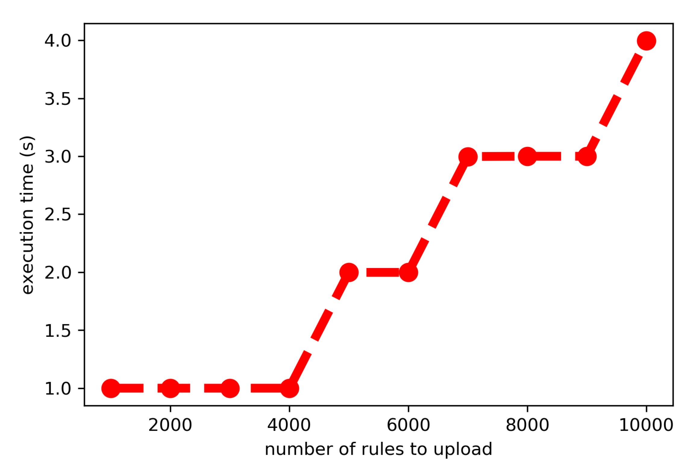
Table 12. The presented verification of the speed of our classification method shows its linear computational complexity.
7. Conclusions
This work is about rule-based decision support systems designed for a Database environment. We present the project in a detailed way, step by step, starting from the generation of decision rules and inserting them into the database with appropriate queries. The project is concluded with the presentation of a query allowing an appropriate classification using the rules stored in the database. The presented scheme allows us to build a real-time working (IF THEN) rule-based classifier. The use of our solution is limited to methods generating IF THEN type rules, whose sets of rules do not contain contradictions or longer rules containing correct shorter ones. Other limitations are mainly due to computational complexity of individual methods-and the level of accuracy of covering the knowledge contained in the decision-making systems by the rules generated. Despite initial results that proved to be very promising a great amount of work is left to be done to evaluate the final performance and determine the application of our new method. This work calls for several perspectives. In future implementation of the presented system in selected mobile devices is planned. We are also going to use the system in real-life data mining projects.
Author Contributions
Conceptualization, P.A., L.R. and O.M.; methodology, software, validation, formal analysis and investigation, P.A. and O.M.; data acquisition and classification P.A., L.R.; resources, P.A. and L.R.; writing—original draft preparation, P.A. and L.R.; writing—review and editing, P.A. and L.R.; funding acquisition, P.A. and L.R. All authors have read and agreed to the published version of the manuscript.
Funding
This research received no external funding.
Acknowledgments
The research has been supported by grant 23.610.007-300 from Ministry of Science and Higher Education of the Republic of Poland.
Conflicts of Interest
The authors declare no conflict of interest.
References
- Shearer, C. The CRISP-DM model: The new blueprint for data mining. J. Data Warehous. 2000, 5, 13–22. [Google Scholar]
- Rissanen, J. Modeling by shortest data description. Automatica 1978, 14, 445–471. [Google Scholar] [CrossRef]
- UCI (University of California at Irvine) Repository. Available online: http://archive.ics.uci.edu./ml/ (accessed on 2 August 2020).
- Pawlak, Z. Rough sets. Int. J. Comput. Inf. Sci. 1982, 11, 341–356. [Google Scholar] [CrossRef]
- RSES. Available online: http://mimuw.edu.pl/logic/~rses/ (accessed on 1 April 2014).
- Skowron, A. Boolean reasoning for decision rules generation. In Proceedings of the ISMIS’93. Lecture Notes in Artificial Intelligence; Springer: Berlin, Germany, 1993; Volume 689, pp. 295–305. [Google Scholar]
- Grzymala–Busse, J.W. LERS–A system for learning from examples based on rough sets. In Intelligent Decision Support: Handbook of Advances and Applications of the Rough Sets Theory; Słowiński, R., Ed.; Kluwer Academic Publishers: Dordrecht, The Netherlands, 1992; pp. 3–18. [Google Scholar]
- Skarek, P.; László, Z.V. Rule-Based Knowledge Representation Using a Database. In Proceedings of the Conference on Artificial Intelligence Applications, Paris, France, 21–22 October 1996. [Google Scholar]
- Lorentzos, N.A.; Yialouris, C.P.; Sideridis, A.B. Time-evolving rule-based knowledge bases. Data Knowl. Eng. 1999, 29, 313–335. [Google Scholar] [CrossRef]
- Abdullah, U.; Sawar, M.J.; Ahmed, A. Design of a Rule Based System Using Structured Query Language. In Proceedings of the 2009 Eighth IEEE International Conference on Dependable, Autonomic and Secure Computing, Chengdu, China, 12–14 December 2009; pp. 223–228. [Google Scholar] [CrossRef]
- Spits Warnars, H.L.H. Classification Rule with Simple Select SQL Statement; National Seminar University of Budi Luhur: Jakarta, Indonesia; University of Budi Luhur: Jakarta, Indonesia, 2010. [Google Scholar]
- Liu, C.; Sakai, H.; Zhu, X.; Nakata, M. On Apriori-Based Rule Generation in SQL—A Case of the Deterministic Information System. In Proceedings of the 2016 Joint 8th International Conference on Soft Computing and Intelligent Systems (SCIS) and 17th International Symposium on Advanced Intelligent Systems (ISIS), Sapporo, Japan, 25–28 August 2016; pp. 178–182. [Google Scholar] [CrossRef]
- Miftakul Amin, M.; Andino, M.; Shankar, K.; Eswaran Perumal, R.; Vidhyavathi, M.; Lakshmanaprabu, S.K. Active Database System Approach and Rule Based in the Development of Academic Information System. Int. J. Eng. Technol. 2018, 95–101. [Google Scholar] [CrossRef]
- Salzberg, S.L. C4.5: Programs for Machine Learning by J. Ross Quinlan; Morgan Kaufmann Publishers: Burlington, MA, USA, 1993; Mach Learn 16, 235–240 (1994). [Google Scholar] [CrossRef]
- Artiemjew, P. On Strategies of Knowledge Granulation with Applications to Decision Systems. Ph.D. Thesis, Polish–Japanese Institute of Information Technology, Warszawa, Polish, 2009. [Google Scholar]
- Mitchell, T. Machine Learning; McGraw-Hill: Englewood Cliffs, NJ, USA, 1997. [Google Scholar]
- Chan, C.C.; Grzymala-Busse, J.W. On the two local inductive algorithms: PRISM and LEM2. Found. Comput. Decis. Sci. 1994, 19, 185–204. [Google Scholar]
- Grzymala-Busse, J.W.; Lakshmanan, A. LEM2 with interval extension: An induction algorithm for numerical attributes. In Proceedings of the Fourth International Workshop on Rough Sets, Fuzzy Sets, and Machine Discovery (RSFD’96); The University of Tokyo: Tokyo, Japan, 1996; pp. 67–76. [Google Scholar]
- Michalski, R.S.; Mozetic, I.; Hong, J.; Lavrac, N. The multi–purpose incremental learning system AQ15 and its testing to three medical domains. In Proceedings of AAAI-86; Morgan Kaufmann: San Mateo, CA, USA, 1986; pp. 1041–1045. [Google Scholar]
- Clark, P.; Niblett, T. The CN2 induction algorithm. Mach. Learn. 1989, 3, 261–283. [Google Scholar] [CrossRef]
- Cendrowska, J. PRISM, an algorithm for inducing modular rules. Int. J. Man Mach. Stud. 1987, 27, 349–370. [Google Scholar] [CrossRef]
- Artiemjew, P. On clasification of data by means of rough mereological granules of objects and rules. In Proceedings of the International Conference on Rough Set and Knowledge Technology RSKT’08, Chengdu, China, 17–19 May 2008; LNAI. Springer: Berlin, Germany, 2008; Volume 5009, pp. 221–228. [Google Scholar]
- Polkowski, L.; Artiemjew, P. Granular Computing in Decision Approximation, An Application of Rough Mereology. In Series: Intelligent Systems Reference Library; Springer: Berlin, Germany, 2015; Volume 77, 452p. [Google Scholar]
Figure 1.
Basic scheme of the database system vs. rule-based knowledge based system.
Figure 1.
Basic scheme of the database system vs. rule-based knowledge based system.
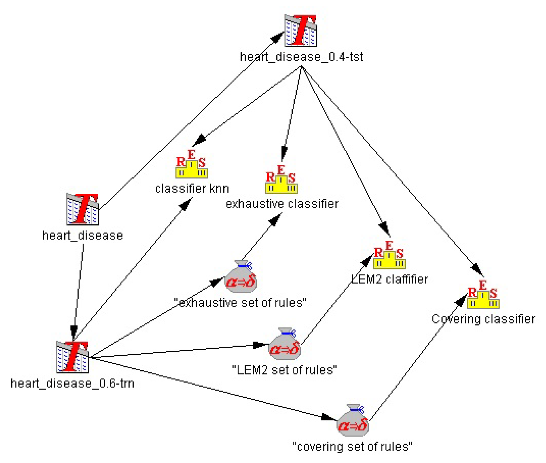
Figure 2.
Considering Train and Test with split ratio
for Statlog (Heart) Data Set (270 objects, 14 attributes) [
3], the Training system has 162 objects, the test system 108. Exemplary classification result; in case of knn we have total and balanced
,
; in case of an exhaustive classifier we have total and balanced
= 0.824,
,
; in case of an LEM2 classifier we have total
, balanced
,
,
; in case of a Covering classifier we have total
, balanced
,
,
.
Figure 3.
The speed of loading rules into the database for batches of 1000, 2000, …, 10,000 rules.
Figure 3.
The speed of loading rules into the database for batches of 1000, 2000, …, 10,000 rules.
Figure 4.
Speed of classification of 1000 random test objects in databases containing from 1000 to 10,000 rules.
Figure 4.
Speed of classification of 1000 random test objects in databases containing from 1000 to 10,000 rules.
Figure 5.
The classification speed of 100 to 1000 test objects by 10,000 rules in the database table.
Figure 5.
The classification speed of 100 to 1000 test objects by 10,000 rules in the database table.
Table 1.
The exemplary decision system .
Table 1.
The exemplary decision system .
| | | | d |
|---|
| red | | |
| green | | |
| blue | | |
Table 2.
The exemplary decision system-for rule induction [
14].
Table 2.
The exemplary decision system-for rule induction [
14].
| Day | Weather | Temperature | Humidity | Wind | Play_Tennis |
|---|
| D1 | Sunny | Hot | High | Weak | No |
| D2 | Sunny | Hot | High | Strong | No |
| D3 | Overcast | Hot | High | Weak | Yes |
| D4 | Rain | Mild | High | Weak | Yes |
| D5 | Rain | Cold | Normal | Weak | Yes |
| D6 | Rain | Cold | Normal | Strong | No |
| D7 | Overcast | Cold | Normal | Strong | Yes |
| D8 | Sunny | Mild | High | Weak | No |
| D9 | Sunny | Cold | Normal | Weak | Yes |
| D10 | Rain | Mild | Normal | Weak | Yes |
| D11 | Sunny | Mild | Normal | Strong | Yes |
| D12 | Overcast | Mild | High | Strong | Yes |
| D13 | Overcast | Hot | Normal | Weak | Yes |
| D14 | Rain | Mild | High | Strong | No |
Table 3.
Examples of real rules-exhaustive algorithm, Statlog (heart) Data Set [
3], Rule statistics: 5352 rules, Support of rules Minimal: 1, Maximal: 32, Mean:
, Length of rule premises, Minimal: 1, Maximal: 6, Mean:
, Distribution of rules among decision classes, Decision class 1: 2732, Decision class 2: 2620.
| (attr1=0)&(attr5=0)&(attr6=0)&(attr8=0)&(attr12=30)=>(attr13=1[32]) |
| (attr1=0)&(attr2=30)&(attr12=30)=>(attr13=1[29]) |
| (attr1=0)&(attr6=0)&(attr10=10)=>(attr13=1[26]) |
| (attr2=40)&(attr6=20)&(attr10=20)&(attr12=70)=>(attr13=2[25]) |
| (attr1=0)&(attr6=0)&(attr8=0)&(attr11=0)=>(attr13=1[25]) |
| (attr1=0)&(attr2=30)&(attr11=0)=>(attr13=1[24]) |
| (attr2=20)&(attr5=0)&(attr10=10)&(attr12=30)=>(attr13=1[22]) |
| (attr1=0)&(attr5=0)&(attr8=0)&(attr10=20)&(attr12=30)=>(attr13=1[20]) |
| (attr1=0)&(attr2=30)&(attr10=10)=>(attr13=1[20]) |
Table 4.
Examples of real rules-LEM2 algorithm, Statlog (heart) Data Set [
3], Rule statistics: 99 rules, Support of rules Minimal: 1, Maximal: 23, Mean:
, Length of rule premises, Minimal: 4, Maximal: 10, Mean:
, Distribution of rules among decision classes, Decision class 1: 43, Decision class 2: 56.
| (attr5=0)&(attr8=0)&(attr12=30)&(attr1=0)&(attr2=30)=>(attr13=1[23]) |
| (attr5=0)&(attr8=0)&(attr12=30)&(attr11=0)&(attr1=0)&(attr6=0)=>(attr13=1[22]) |
| (attr5=0)&(attr8=0)&(attr12=30)&(attr10=10)&(attr6=0)&(attr1=0)=>(attr13=1[21]) |
| (attr5=0)&(attr1=10)&(attr2=40)&(attr12=70)&(attr8=10)&(attr10=20)&(attr6=20)=>(attr13=2[13]) |
| (attr5=0)&(attr1=10)&(attr2=40)&(attr8=10)&(attr6=20)&(attr11=10)=>(attr13=2[12]) |
| (attr8=0)&(attr1=10)&(attr11=0)&(attr5=10)=>(attr13=1[11]) |
| (attr5=0)&(attr8=0)&(attr12=30)&(attr11=0)&(attr6=20)&(attr1=0)&(attr10=20)=>(attr13=1[9]) |
Table 5.
Examples of real rules-Sequential covering algorithm, Statlog (heart) Data Set [
3], Rule statistics: 199 rules, Support of rules Minimal: 1, Maximal: 7, Mean:
, Length of rule premises, Minimal: 1, Maximal: 1, Mean: 1, Distribution of rules among decision classes, Decision class 1: 106, Decision class 93: 56.
| (attr7=1720)=>(attr13=1[7]) |
| (attr7=1780)=>(attr13=1[5]) |
| (attr4=2040)=>(attr13=1[4]) |
| (attr4=2110)=>(attr13=1[4]) |
| (attr4=2260)=>(attr13=1[4]) |
| (attr4=2820)=>(attr13=2[4]) |
| (attr7=1510)=>(attr13=1[4]) |
| (attr7=1790)=>(attr13=1[4]) |
Table 6.
An example of how to upload rules into the database.
Table 6.
An example of how to upload rules into the database.
| Original Rule | SQL QUERY |
|---|
|
|
|
|
Table 7.
The demonstration problem to be solved.
Table 7.
The demonstration problem to be solved.
| Test Object |
|---|
Weather is Sunny
Temperature is Mild
Humidity is Normal
Wind is Weak |
Table 8.
The demonstration of the query used to classify the test object.
Table 8.
The demonstration of the query used to classify the test object.
| Decision-Making by Single Query |
|---|
|
Table 9.
Sample of random rules created by the generator for benchmarking purposes. In experiments we use 10,000 randomly generated rules.
Table 9.
Sample of random rules created by the generator for benchmarking purposes. In experiments we use 10,000 randomly generated rules.
| Rules in the Form of a Database Query |
|---|
| INSERT INTO rules(Weather,Temperature,Humidity,Wind,Play_Tennis,length,support)VALUES(’Rain’,’-’,’-’,’-’,’Yes’,4,5);
|
| INSERT INTO rules(Weather,Temperature,Humidity,Wind,Play_Tennis,length,support)VALUES(’Overcast’,’Mild’,’-’,’Strong’,’No’,1,4);
|
| INSERT INTO rules(Weather,Temperature,Humidity,Wind,Play_Tennis,length,support)VALUES(’Overcast’,’Cold’,’Normal’,’Strong’,’Yes’,2,4);
|
Table 10.
Creating tables to test the classification process, In experiments we upload to Tables 10000 randomly generated rules.
Table 10.
Creating tables to test the classification process, In experiments we upload to Tables 10000 randomly generated rules.
| Creating Database Tables |
|---|
| CREATE TABLE rules1000(Weather TEXT, Temperature TEXT, Humidity TEXT, Wind TEXT, Play_Tennis TEXT, length int, support int);
|
| CREATE TABLE rules2000(Weather TEXT, Temperature TEXT, Humidity TEXT, Wind TEXT, Play_Tennis TEXT, length int, support int);
|
| CREATE TABLE rules3000(Weather TEXT, Temperature TEXT, Humidity TEXT, Wind TEXT, Play_Tennis TEXT, length int, support int);
|
Table 11.
Sample of random generated classification query.
Table 11.
Sample of random generated classification query.
| Classification Based on Single Query |
|---|
SELECT Play_Tennis FROM rules10000
WHERE Weather in(’Sunny’,’-’)
AND Temperature in(’Mild’,’-’ )
AND Humidity in(’Normal’,’-’)
AND Wind in(’Weak’,’-’)
GROUP BY Play_Tennis
ORDER BY SUM(support∗length) DESCLIMIT 1; |
Table 12.
The code for calculating the speed of execution of database operations.
Table 12.
The code for calculating the speed of execution of database operations.
| SET @start_time = (TIMESTAMP(NOW()) * 1000000 + MICROSECOND(NOW(6))); |
| select @start_time; |
| ... |
| SET OF DATABASE QUERIES |
| ... |
| SET @end_time = (TIMESTAMP(NOW()) * 1000000 + MICROSECOND(NOW(6))); |
| select @end_time; |
| select (@end_time-@start_time)/1000; |
| Publisher’s Note: MDPI stays neutral with regard to jurisdictional claims in published maps and institutional affiliations. |
© 2020 by the authors. Licensee MDPI, Basel, Switzerland. This article is an open access article distributed under the terms and conditions of the Creative Commons Attribution (CC BY) license (http://creativecommons.org/licenses/by/4.0/).


