NFV-Enabled Efficient Renewable and Non-Renewable Energy Management: Requirements and Algorithms


Abstract
1. Introduction
- The description of an NFV-enabled energy management ecosystem, the requirements, and the mechanisms to perform adaptive energy management of available supply, whether or not it is renewable.
- The ILP formulation of the adaptive energy management model.
- An exact algorithmic strategy, defined as OptTs, which based on a brute-force search combinatorial analysis solves the ILP optimally.
- The discussion of possible algorithms to tackle the hardness of the ILP and the computational complexity of OptTs.
- A heuristic solution defined as FastTs that based on a prepartitioning method produces solutions with a reduced running time (as compared to the optimal) and is applicable to large-scale environments.
- The evaluation of the strategies OptTs and FastTs through extensive simulations in order to confirm the improvements in energy consumption and demand processing.
2. Related Work
2.1. ICT-Based Energy Management Systems
2.2. Features of Our Proposal
3. Adaptive Energy Managements: Requirements, Components, and Mechanisms
3.1. Problem Statement and Overview of the Energy Management Ecosystem
3.2. Requirements for Adaptive Energy Management
- Adaptive consumption of available energy: for optimal use of available energy, the consumption pattern must be adapted to the existing energy resources at all times, whether or not they are deterministic (this is the case when the energy comes from renewable sources). In order to carry out this procedure, the ECs must collaborate with the ES and be willing to shift the execution of services (i.e., advance or delay consumption) according to availability. In this way, the ES can stimulate consumption or propose the deferment of services during periods of surplus or shortage, respectively. The cooperation between ES and ECs is defined by means of contracts in which technical (service parameters) and economic (pricing schemes) aspects are established. Technically, the consumption adaptation procedure is executed through management mechanisms, such as those described in Section 3.3.3.
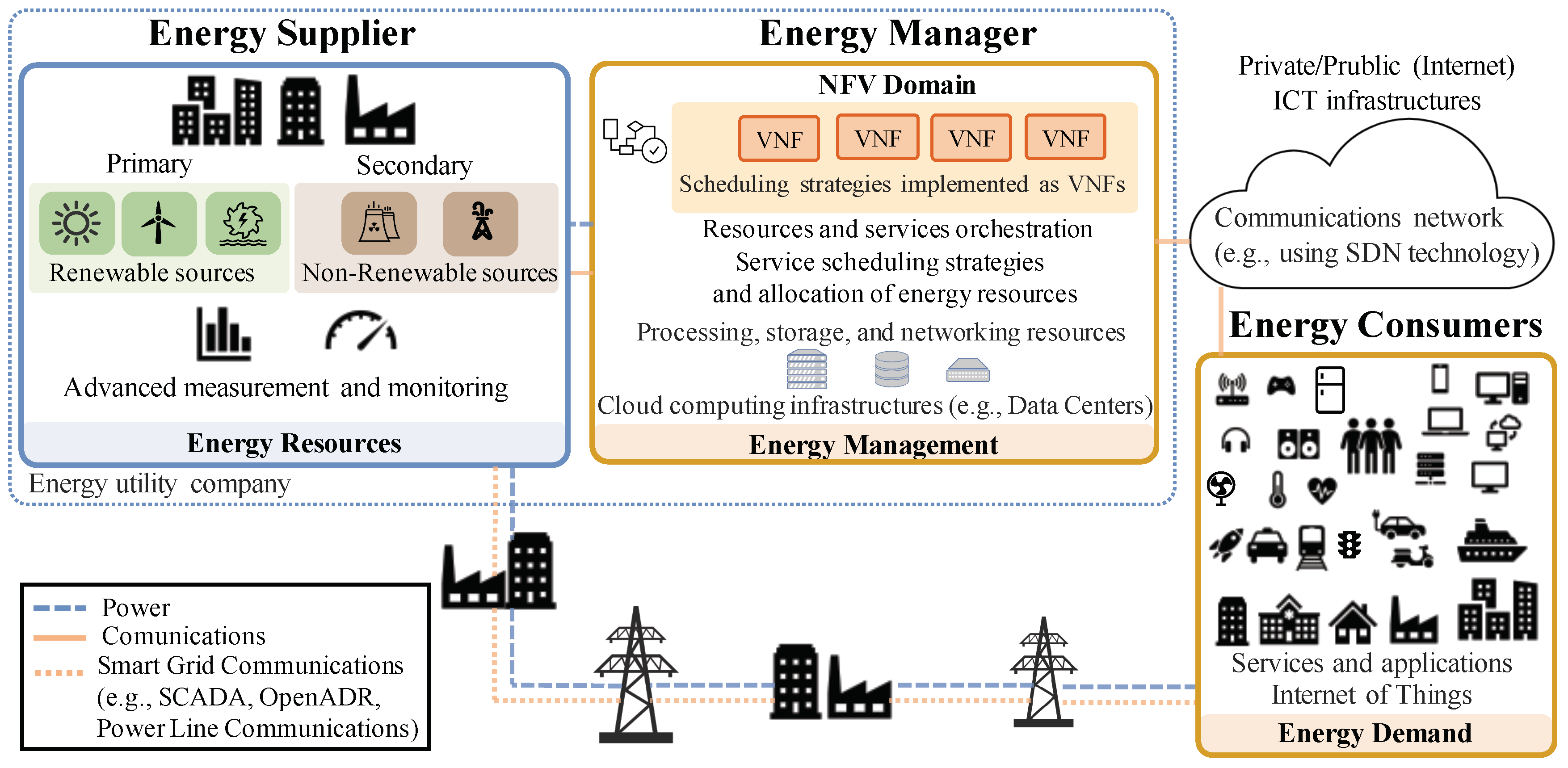
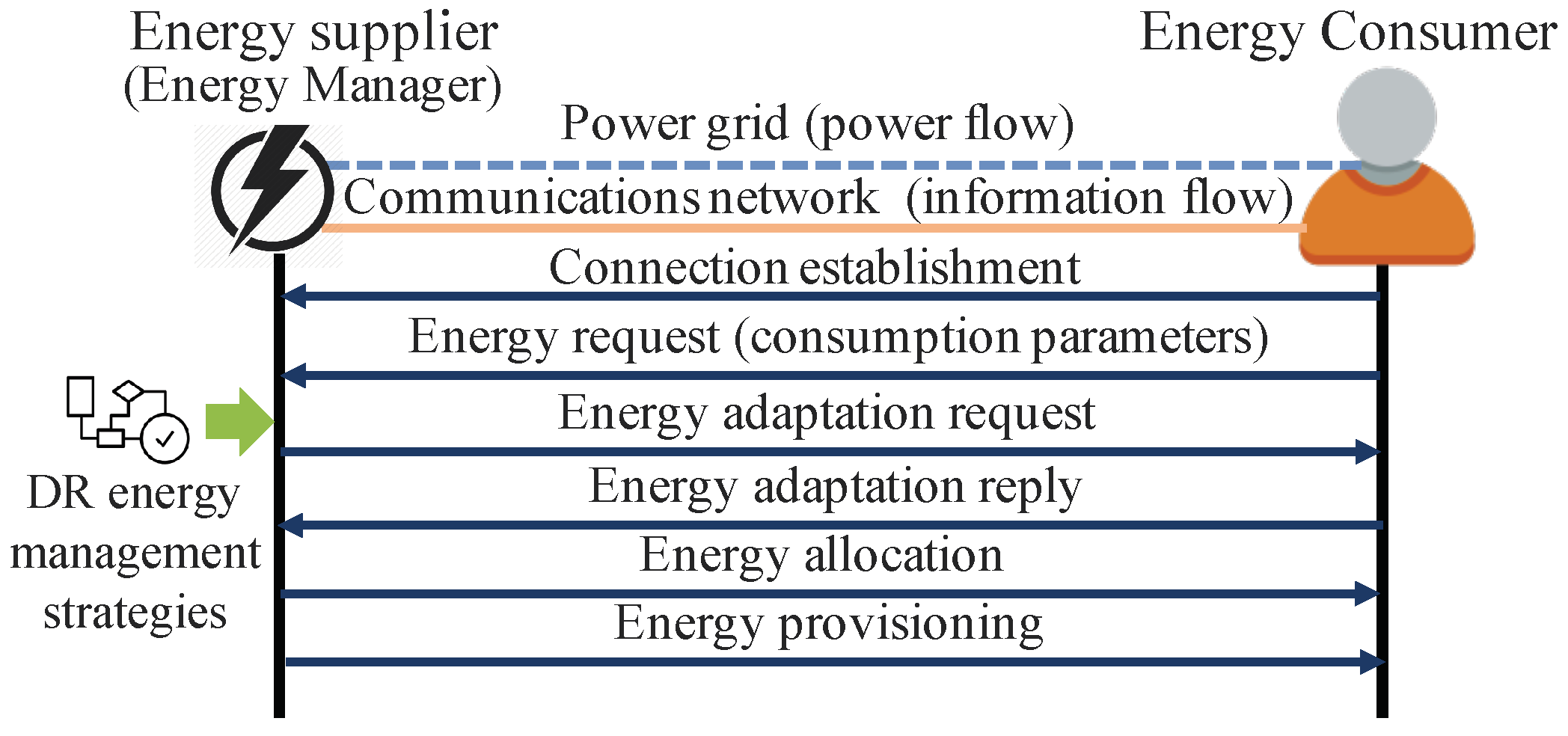
- Customer-side participation in the energy management process: in an adaptive energy management system, the ECs must interact with the ES. The level of interaction between these stakeholders can be fully automated or may require end-user participation, depending on the characteristics of each service and application environment (e.g., residential, industrial, or public infrastructures scenarios). In summary, each time an EC requests energy for service execution, a handshake process must be established with the ES (technically, this process is performed by the EM; see Figure 1), in which information on energy demands and available resources is exchanged. With the collected information, the ES (technically, the EM) must perform the corresponding calculations in order to inform the ECs of the consumption conditions (i.e., the services to which energy can be allocated and their respective execution time). This procedure is described in more detail in Section 3.3.3. Regarding the functional requirement, in order for ECs to participate in the energy management ecosystem, they must have automated IoT capabilities to allow communication (with the ES) and manageability (activation/deactivation of consumption). Currently, a large number of devices are manufactured with embedded communication systems. In addition, if needed, affordable platforms (e.g., Arduino, Raspberry, or ESP32 platforms) can be integrated into virtually any device in order to provide connectivity and automation capabilities. In this context, different protocols, interfaces, and IoT solutions can be used for different purposes and applications. However, a discussion of specific solutions for these purposes is beyond the scope of this paper.
- ICT infrastructure for the establishment of communication between components: the communications infrastructure is a fundamental component of an adaptive energy management system [10]. This infrastructure must enable the reliable and secure exchange of information and instructions related to energy management (i.e., information on service parameters, notifications, and consumption indications). Different communication technologies can be used to interconnect the components (ES-EM-ECs), as shown in Figure 1. However, the most suitable option of an underlying network to communicate the different stakeholders is the Software Defined Networking (SDN) technology due to complementarity with the NFV realm [24]. Regarding the ownership, operation, and maintenance aspects of the ICT infrastructure, different options can be analyzed. In the first instance, the ICT infrastructure could be leased by energy suppliers and distributors, but it is expected that, with the massive connectivity and IoT and IoE trends, the energy sector will invest and deploy sophisticated communications networks. The current smart grids could be used as a baseline infrastructure for this purpose.
- ICT infrastructure for performing management strategies: the ecosystem for adaptive energy management requires an entity that coordinates all actions between the ES and the ECs. In the scheme presented in Figure 1 these functionalities are performed by the EM; this component is normally part of the ES and is in charge of performing all calculations and executing all strategies (algorithms) that are associated with energy management from ES to ECs. In this regard, Ref. [5] demonstrates that NFV technology deployed on cloud computing infrastructures is an ideal solution to meet the scalability, flexibility, and reconfigurability requirements of adaptive energy consumption. An NFV-enabled EM can grow proportionally (increase in computing, storage, and networking resources) according to the varied requirements of the ECs, and it can dispose of the Management and Orchestration (MANO) entities [6], so that all the components of the generation and consumption ecosystem work in a coordinated manner. Thanks to NFV technology, the manageability of the ECs through the underlying network (e.g., SDN) is separated (abstracted) from the functionality (i.e., management strategies), a feature that enables energy management in different scenarios (e.g., HEMS, companies, or smart cities).
- Primary use of renewable energy sources and control of their contribution: although this requirement is not indispensable in optimizing the consumption of the available supply, our proposal encourages the primary use of green energy and the transition to 100% renewable energy systems, as an emissions-aware and sustainable solution. In this regard, the proposed energy management mechanisms, such as workload scheduling through time-shifting capabilities, prioritization in energy supply, or rejection of energy demands if necessary, enable the optimal use of the sporadic energy capacity from green sources such as solar or wind. Furthermore, given that the change towards zero-emission energy systems is gradual and it requires the co-existence of both renewable and non-renewable sources, controlling the contribution of each source according to its availability and need is an important parameter in the operation of the ES.
3.3. Components of the NFV-Enabled Ecosystem and Proposed Energy Management Mechanisms
3.3.1. Energy Supplier
3.3.2. Energy Consumers
3.3.3. NFV-Enabled Energy Manager and Mechanisms for Adaptive Consumption
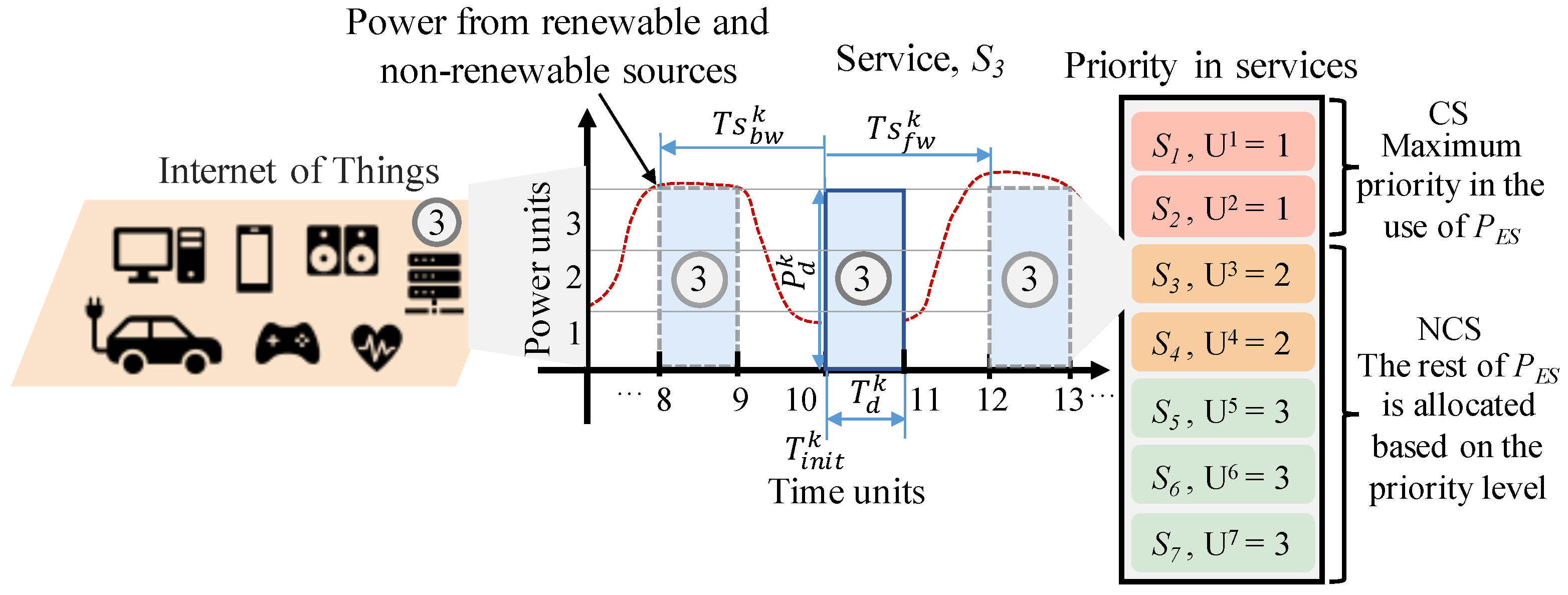
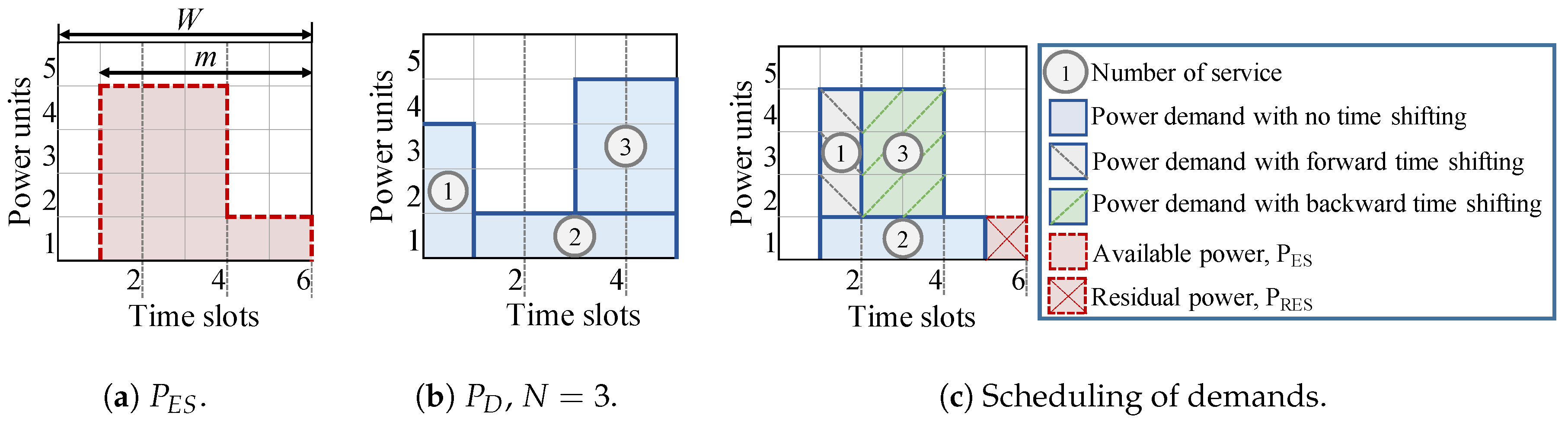
- Adaptation of consumption to availability by exploiting time-shifting capabilities of services: the adaptation of the consumption pattern to the availability, is achieved with the use of temporary displacement on the service. Thus, a service k () can be affected by a time-shifting () forward (i.e., ) or backward (i.e., ) within a finite interval of time horizon W. These parameters are independent for each service , and the management strategies (algorithms as shown in Section 5) deployed in the NFV domain determine the efficient (optimal) scheduling of services to optimize the use of .
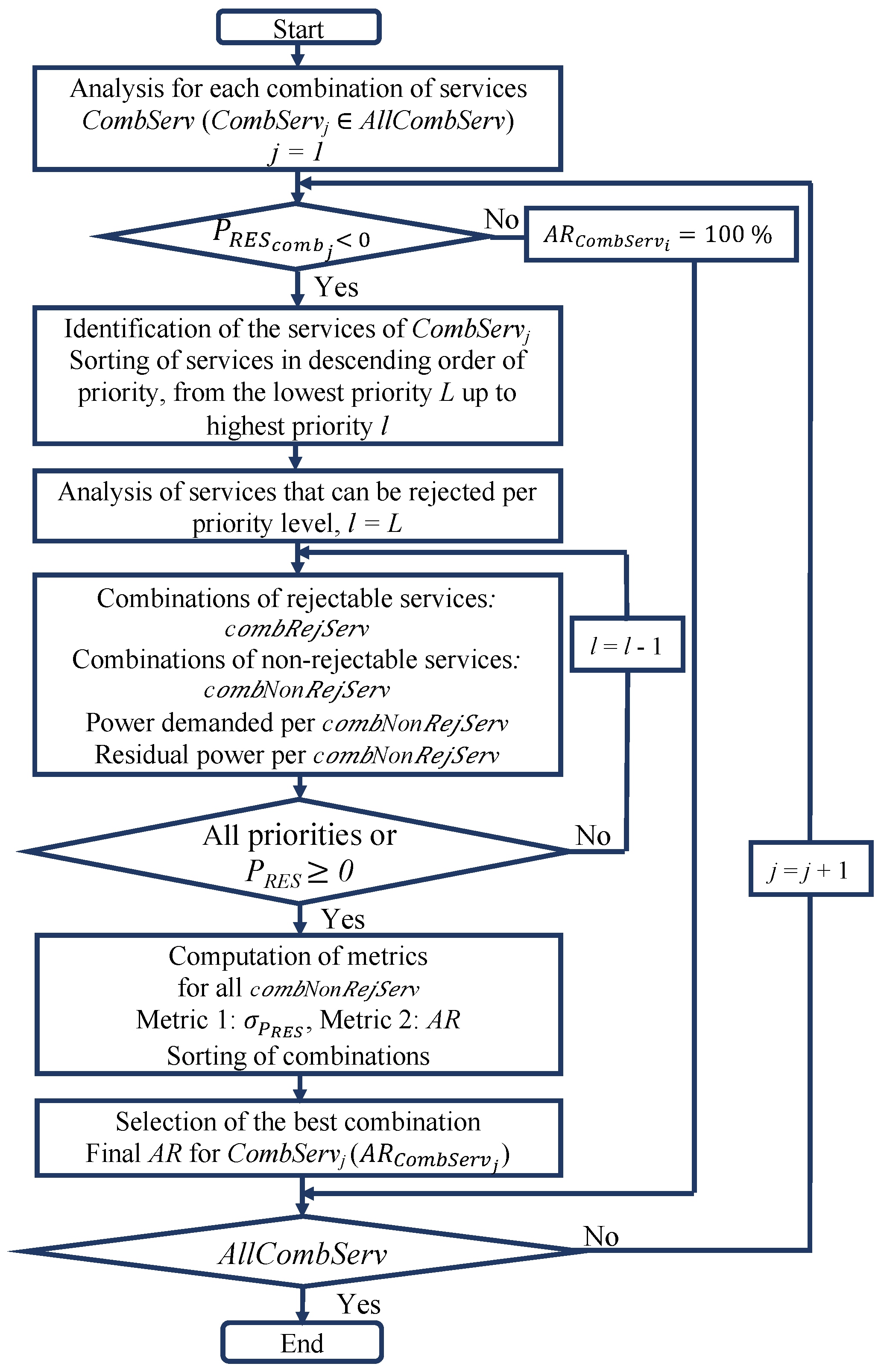
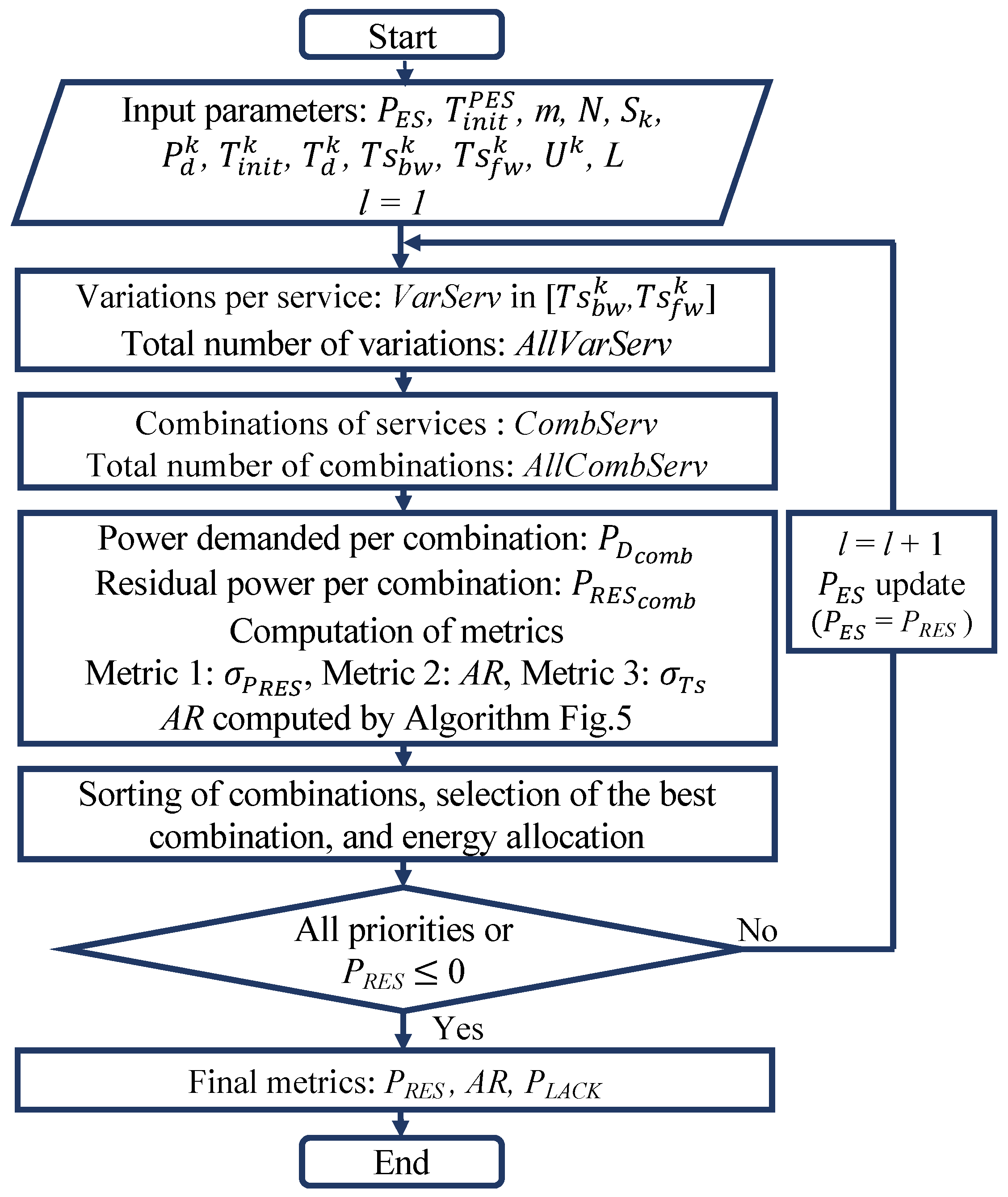
- Prioritization in energy distribution and rejection of demands: if , the the EM allocates the energy resources to the services according to the category to which they belong, i.e., the supply is prioritized for the execution of CS (). The remaining energy is allocated to the NCS in decreasing order according to their priority level (from down to ). Thus, services with a lower priority level are more likely to be unprocessed or rejected. If all services have an equal level of priority, the service scheduling algorithms aim to use energy as efficiently as possible and, second, to try to meet as many demands (services) as possible. This procedure is explained in detail in the algorithm in Figure 3. Other alternatives that could be analyzed in future work, if , are the degradation of the quality of services (e.g., decrease in display brightness of a device), and the use of energy stored in batteries during energy surplus periods. A service is completely defined by the parameters that are listed in Table 3, and an example is illustrated in Figure 4.
4. ILP Problem Formulation: OptTs
4.1. Objective Function
Domain Constraints
4.2. Capacity Constraint
4.3. Time Constraints
4.4. Hardness of the Problem
5. Exact Solution: OptTs
5.1. Metrics
5.1.1. Standard Deviation of Residual Power ()
5.1.2. Acceptance Ratio ()
5.1.3. Standard Deviation of Time-Shifting ()
5.2. Optimal Power Management Strategy OptTs
5.2.1. Variations Per Service
5.2.2. Combinations of Services and Computation of Metrics
5.2.3. Sorting of Combinations and Selection of the Best Combination
5.2.4. Iterative Analysis of Priorities
5.3. Complexity Analysis of OptTs
6. Analysis of Heuristic Strategies
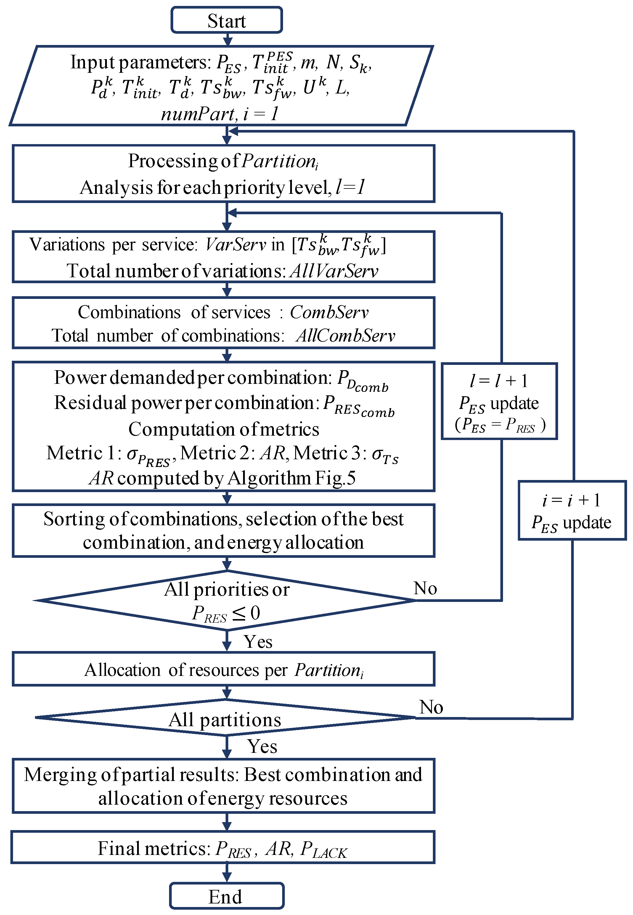
7. Heuristic Solution: FastTs
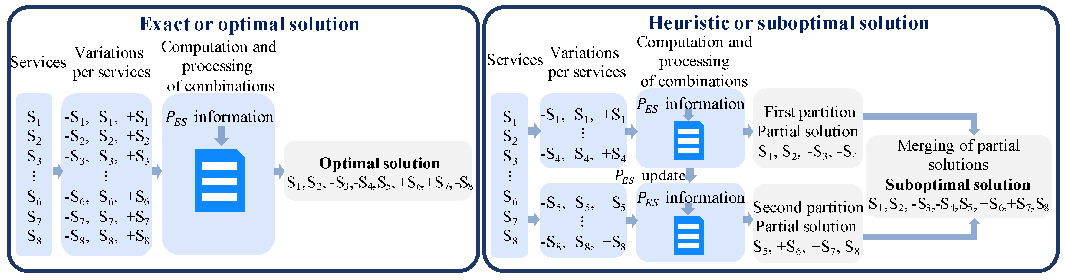
7.1. Suboptimal Power Strategy FastTs
7.1.1. Prepartition Phase
7.1.2. Computation of Combinations Per Partition
7.1.3. Iterative Process
7.1.4. Merging of Partial Solution
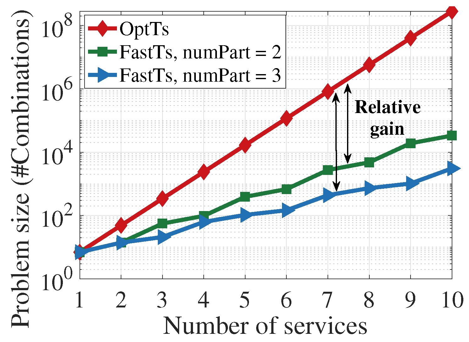
7.2. Complexity Analysis of FastTs
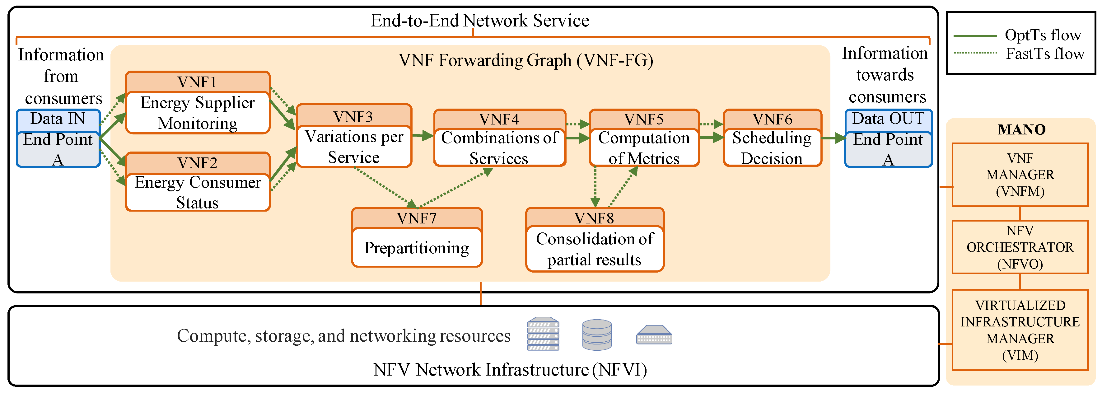
8. Energy Management Algorithmic Strategies a Service Function Chains
- : - - - - - .
- : - - - - - - - - .
9. Evaluation
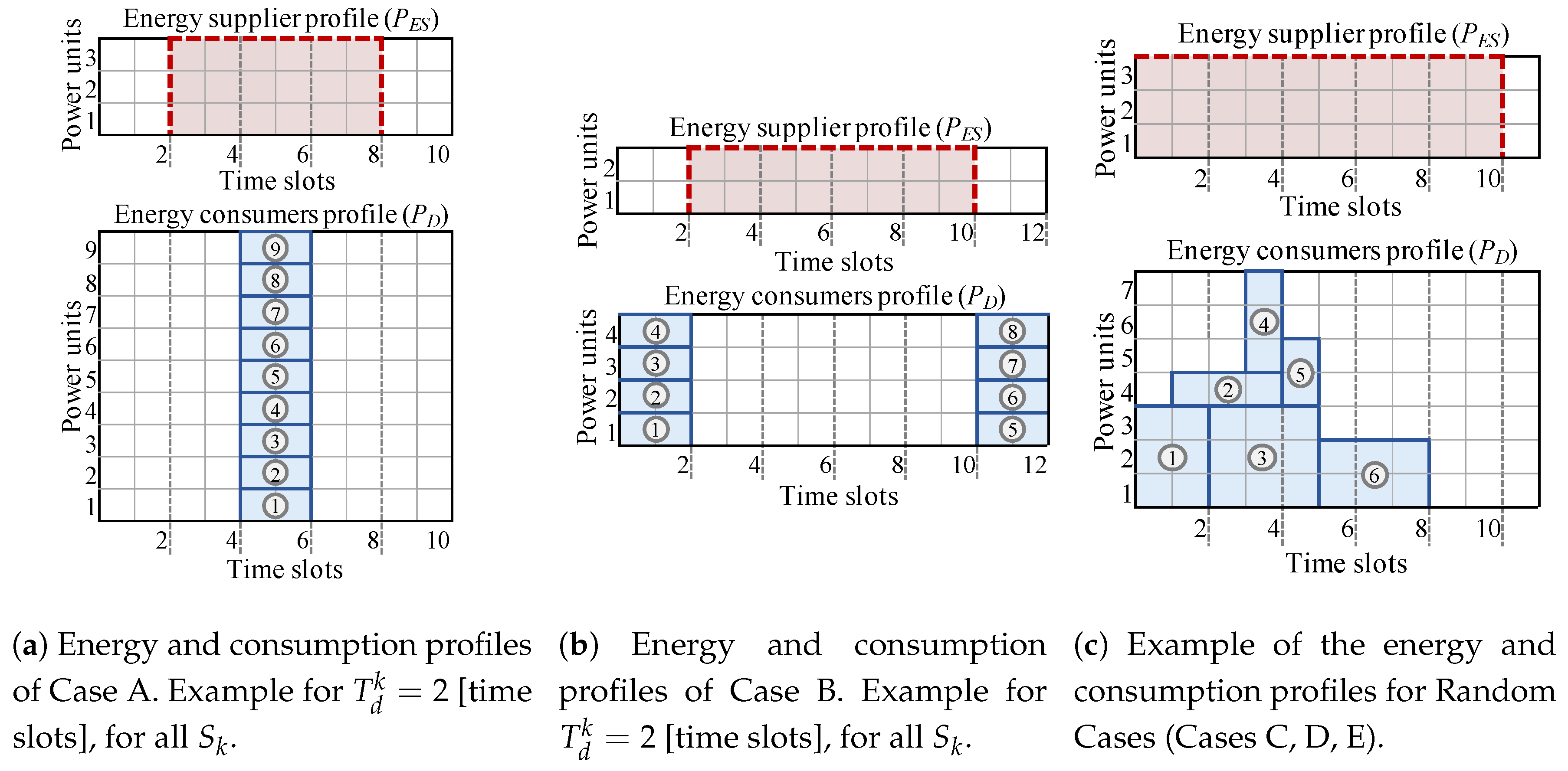
9.1. Case Studies
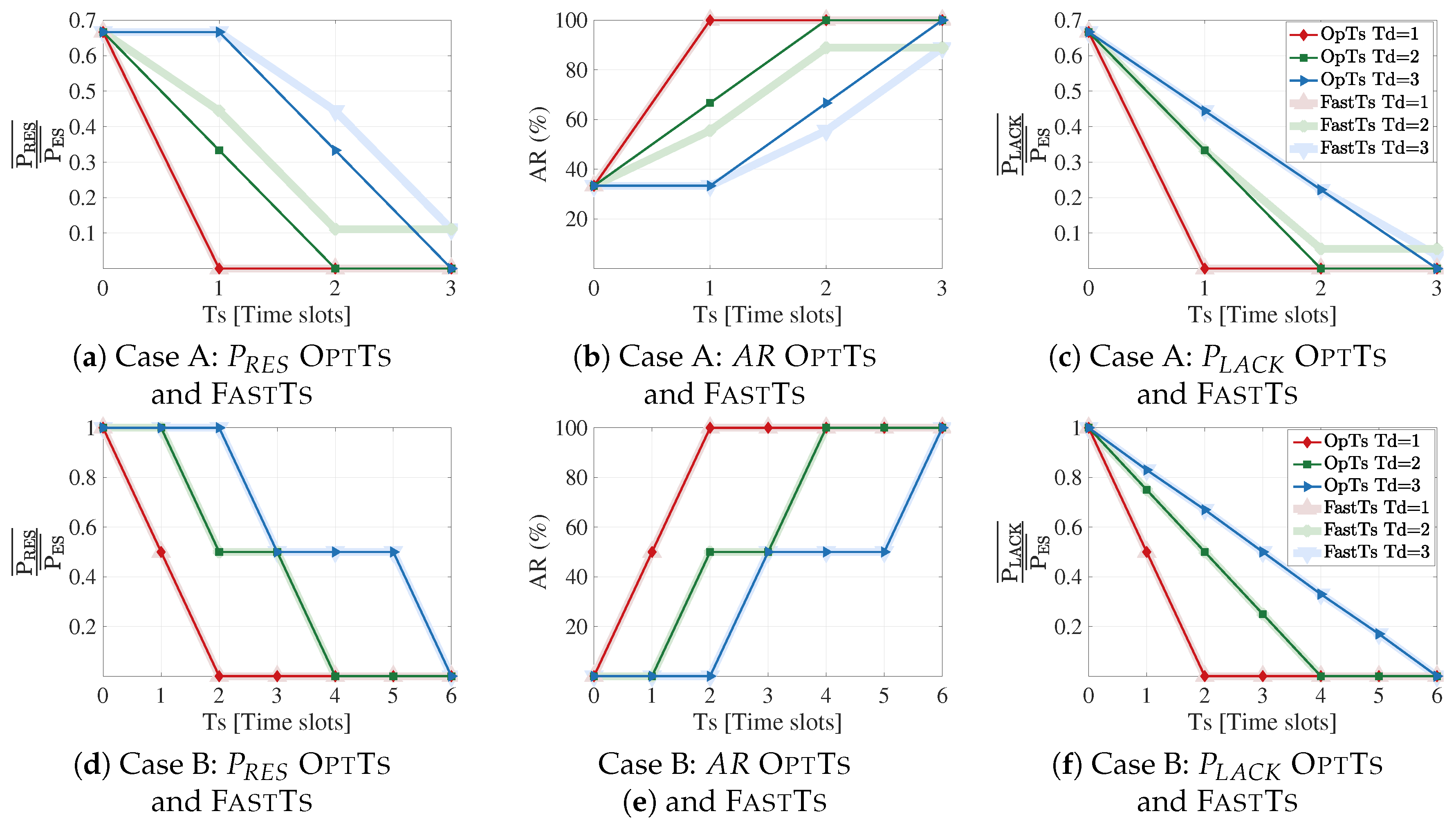
9.2. Analysis for Small-Scale Scenarios
9.2.1. Results in Small-Scale Scenarios
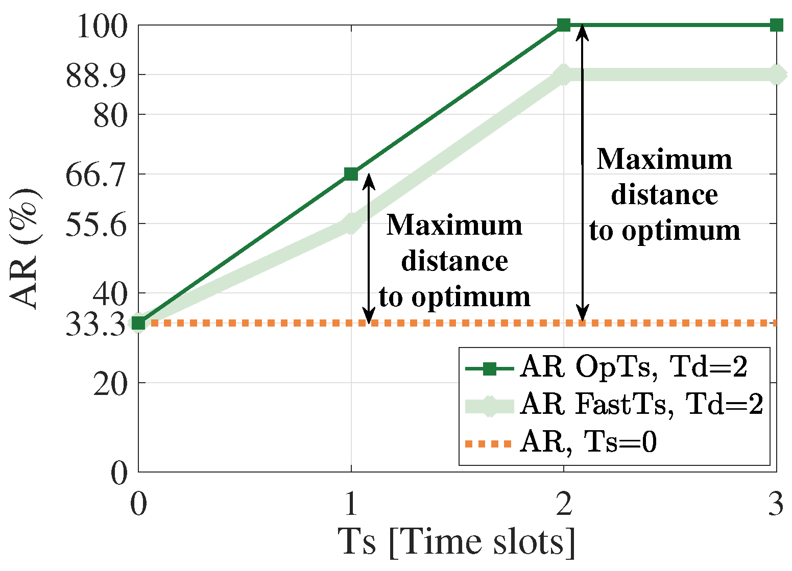
9.2.2. Comparison between OptTs and FastTs
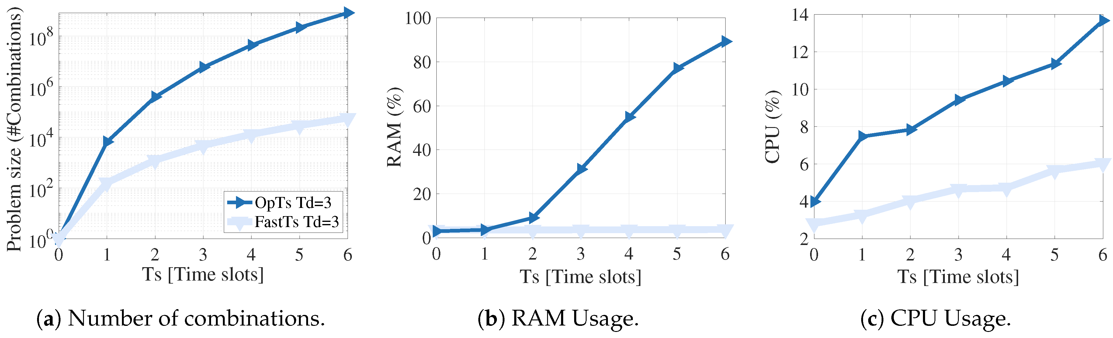
9.2.3. Running Time Analysis
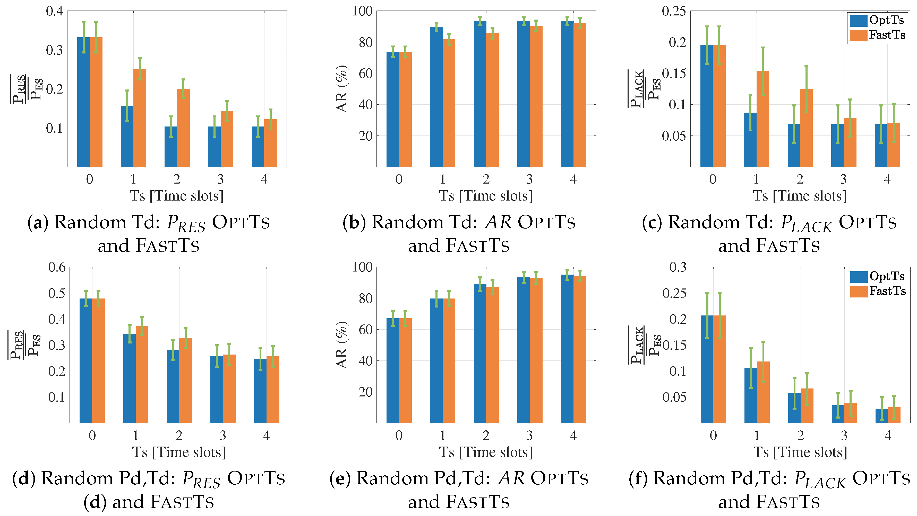
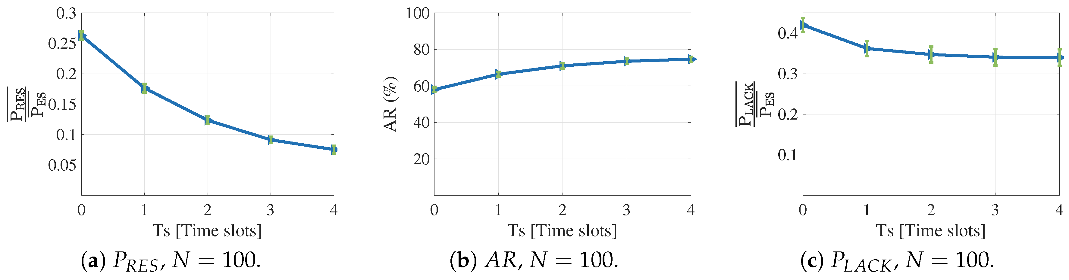
9.3. Analysis for Large-Scale Scenarios
Results Large-Scale Scenarios
9.4. Summary of Results
10. Conclusions
Author Contributions
Funding
Acknowledgments
Conflicts of Interest
References
- Global e-Sustainability Initiative. SMARTer2030, ICT Solutions for 21st Century Challenges; GeSI, Accenture Strategy: Brussels, Belgium, 2015. [Google Scholar]
- Lima, J.M. Data centres of the World Will Consume 1/5 of Earth’s Power by 2025; Technical Report; Euromoney Institutional Investor PLC: London, UK, 2017. [Google Scholar]
- Carrasco, J.M.; Garcia Franquelo, L.; Bialasiewicz, J.T.; Galván, E.; Portillo Guisado, R.C.; Martín Prats, M.d.l.Á.; León, J.I.; Moreno-Alfonso, N. Power-electronic systems for the grid integration of renewable energy sources: A survey. IEEE Trans. Ind. Electron. 2006, 53, 1002–1016. [Google Scholar] [CrossRef]
- Medina, J.; Muller, N.; Roytelman, I. Demand response and distribution grid operations: Opportunities and challenges. IEEE Trans. Smart Grid 2010, 1, 193–198. [Google Scholar] [CrossRef]
- Tipantuña, C.; Hesselbach, X. NFV/SDN Enabled Architecture for Efficient Adaptive Management of Renewable and Non-renewable Energy. IEEE Open J. Commun. Soc. 2020, 1, 357–380. [Google Scholar] [CrossRef]
- ETSI. Network Functions Virtualisation, An Introduction, Benefits, Enablers, Challenges & Call for Action. ETSI White Pap. 2012, 1–16. [Google Scholar]
- Shakerighadi, B.; Anvari-Moghaddam, A.; Vasquez, J.C.; Guerrero, J.M. Internet of things for modern energy systems: State-of-the-art, challenges, and open issues. Energies 2018, 11, 1252. [Google Scholar] [CrossRef]
- Cisco, V. Cisco visual networking index: Forecast and trends, 2017–2022. White Pap. 2018, 1, 1. [Google Scholar]
- Zhou, K.; Yang, S.; Shao, Z. Energy internet: The business perspective. Appl. Energy 2016, 178, 212–222. [Google Scholar] [CrossRef]
- Huang, B.; Bai, X.; Zhou, Z.; Cui, Q.; Zhu, D.; Hu, R. Energy informatics: Fundamentals and standardization. ICT Express 2017, 3, 76–80. [Google Scholar] [CrossRef]
- Ghatikar, G.; Ganti, V.; Matson, N. Demand Response Opportunities and Enabling Technologies for Data Centers: Findings from Field Studies. Lawrence Berkeley Natl. Lab. 2012, LBNL-5763E, 1–48. [Google Scholar]
- Wei, M.; Hong, S.H.; Alam, M. An IoT-based energy-management platform for industrial facilities. Appl. Energy 2016, 164, 607–619. [Google Scholar] [CrossRef]
- AlFaris, F.; Juaidi, A.; Manzano-Agugliaro, F. Intelligent homes’ technologies to optimize the energy performance for the net zero energy home. Energy Build. 2017, 153, 262–274. [Google Scholar] [CrossRef]
- Allience, O. OpenADR 2.0 Profile Specification B Profile; Technical Report; OpenADR Alliance: Morgan Hill, CA, USA, 2013. [Google Scholar]
- Basmadjian, R.; Botero, J.F.; Giuliani, G.; Hesselbach, X.; Klingert, S.; De, H. Making Data Centres Fit for Demand Response: Introducing GreenSDA and GreenSLA Contracts. IEEE Trans. Smart Grid 2017, 9, 3453–3464. [Google Scholar] [CrossRef]
- Niedermeier, M.; De Meer, H. Constructing dependable smart grid networks using network functions virtualization. J. Netw. Syst. Manag. 2016, 24, 449–469. [Google Scholar] [CrossRef]
- Mijumbi, R. On the energy efficiency prospects of network function virtualization. arXiv 2015, arXiv:1512.00215. [Google Scholar]
- GreenTouch. G.W.A.T.T. (Global What if Analyzer of NeTwork Energy ConsumpTion). OnlineWeb Tool to Provide an End-to-End View of the GreenTouch Portfolio of Technologies and Solutions on Network Energy Consumption. 2015. Available online: http://alu-greentouch-dev.appspot.com/intro/1 (accessed on 1 September 2020).
- Li, X.; Ferdous, R.; Chiasserini, C.F.; Casetti, C.E.; Moscatelli, F.; Landi, G.; Casellas, R.; Sakaguchi, K.; Chundrigar, S.B.; Vilalta, R.; et al. Novel Resource and Energy Management for 5G integrated backhaul/fronthaul (5G-Crosshaul). In Proceedings of the 2017 IEEE International Conference on Communications Workshops (ICC Workshops), Paris, France, 21–25 May 2017; pp. 778–784. [Google Scholar]
- Al-Quzweeni, A.N.; Lawey, A.Q.; Elgorashi, T.E.; Elmirghani, J.M. Optimized energy aware 5G network function virtualization. IEEE Access 2019, 7, 44939–44958. [Google Scholar] [CrossRef]
- Tipantuña, C.; Hesselbach, X.; Sánchez-Aguero, V.; Valera, F.; Vidal, I.; Nogales, B. An NFV-Based Energy Scheduling Algorithm for a 5G Enabled Fleet of Programmable Unmanned Aerial Vehicles. Wirel. Commun. Mob. Comput. 2019, 2019, 4734821. [Google Scholar] [CrossRef]
- Tsoukalas, L.; Gao, R. From smart grids to an energy internet: Assumptions, architectures and requirements. In Proceedings of the 2008 Third International Conference on Electric Utility Deregulation and Restructuring and Power Technologies, Nanjing, China, 6–9 April 2008; pp. 94–98. [Google Scholar]
- Strasser, T.; Andrén, F.; Kathan, J.; Cecati, C.; Buccella, C.; Siano, P.; Leitao, P.; Zhabelova, G.; Vyatkin, V.; Vrba, P.; et al. A review of architectures and concepts for intelligence in future electric energy systems. IEEE Trans. Ind. Electron. 2014, 62, 2424–2438. [Google Scholar] [CrossRef]
- ETSI. Network Functions Virtualisation (NFV); Ecosystem; Report on SDN Usage in NFV Architectural Framework. ETSI Netw. Funct. Virtualisat. Ind. Specif. Group GS NFV-EVE 2015, 5, V1. [Google Scholar]
- Keles, C.; Kaygusuz, A.; Alagoz, B.B. Multi-source energy mixing by time rate multiple PWM for microgrids. In Proceedings of the 4th International Istanbul Smart Grid Congress and Fair, ICSG 2016, Istanbul, Turkey, 20–21 April 2016. [Google Scholar] [CrossRef]
- Garey, M.R.; Johnson, D.S. Computers and Intractability: A Guide to the Theory of NP-Completeness, 1st ed.; WH Free. Co.: San Francisco, CA, USA, 1979; p. 340. [Google Scholar]
- Pisinger, D. Algorithms for Knapsack Problems; Dept. of Computer Science, University of Copenhagen: København, Denmark, 1995. [Google Scholar]
- Vazirani, V.V. Approximation Algorithms; Springer Science & Business Media: Berlin/Heidelberg, Germany, 2013. [Google Scholar]
- Cormen, T.H.; Leiserson, C.E.; Rivest, R.L.; Stein, C. Introduction to Algorithms; MIT Press: Cambridge, MA, USA, 2009. [Google Scholar]
- Shao, B.B.; Rao, H.R. A parallel hypercube algorithm for discrete resource allocation problems. IEEE Trans. Syst. Man Cybern. Part Syst. Hum. 2006, 36, 233–242. [Google Scholar] [CrossRef]
- Tomassilli, A.; Huin, N.; Giroire, F.; Jaumard, B. Energy-Efficient Service Chains with Network Function Virtualization; HAL: Houston, TX, USA, 2016. [Google Scholar]
- Kim, S.; Han, Y.; Park, S. An energy-aware service function chaining and reconfiguration algorithm in NFV. In Proceedings of the 2016 IEEE 1st International Workshops on Foundations and Applications of Self* Systems (FAS* W), Augsburg, Germany, 12–16 September 2016; pp. 54–59. [Google Scholar]
- Ayan, O.; Turkay, B. Energy Management Algorithm for Peak Demand Reduction. In Proceedings of the 2018 20th International Symposium on Electrical Apparatus and Technologies (SIELA), Bourgas, Bulgaria, 3–6 June 2018; pp. 1–4. [Google Scholar]


| Acronym | Definition | Acronym | Definition |
|---|---|---|---|
| CS | Critical Services | IoE | Internet of Energy |
| DC | Data Center | IoT | Internet of Things |
| DR | Demand Response | MANO | Management and Orchestration |
| EC | Energy Consumer | NCS | Non-Critical Services |
| EM | Energy Manager | NFV | Network Functions Virtualization |
| ES | Energy Supplier | NFVO | NFV Orchestrator |
| HEMS | Home Energy Management System | SDN | Software Defined Network |
| ICT | Information and Communications Technologies | SFC | Service Function Chain |
| ILP | Integer Linear Programming | VNF | Virtual Network Function |
| Notation | Definition | Notation | Definition |
|---|---|---|---|
| l | Priority identifier, | Lifetime of the service k | |
| L | Number of priority levels | Starting time of the service k | |
| m | Time interval where | Starting time of | |
| N | Number of services | General or maximum time-shifting value | |
| Optimal or exact algorithmic strategy | Backward time-shifting of service k | ||
| Power demanded by service k with priority l | Forward time-shifting of service k | ||
| Aggregated power demanded | Priority of service k | ||
| Available power in the system | W | Maximum time horizon in the system | |
| Power from Non-Renewable sources | Weight associated to renewable energy | ||
| Power from Renewable sources | Standard deviation of | ||
| Service identifier, | Standard deviation of |
| Parameter | Description | Unit/Comment |
|---|---|---|
| N | Number of services | Integer number |
| Service identifier | ||
| L | Number of priority levels | Integer number |
| l | Priority identifier | |
| Power demanded by service k | Power units | |
| Starting time of service k | Time units | |
| Lifetime of service k | Time units | |
| Backward time-shifting of service k | Time units | |
| Forward time-shifting of service k | Time units | |
| Priority of service k | Integer number |
| Strategy/Technique | General Description | Features and Challenges |
|---|---|---|
| Pre-partitionig Strategy | Strategy based on a divide-and-conquer method. In this strategy, the original set of N is divided into subsets. The OptTs strategy is applied to each of these subsets. This operation reduces the complexity by reducing the and the in each processed subset. This heuristic strategy iteratively processes all sub-problems, and the solution is obtained as a combination of partial solutions. |
|
| Greedy Approach | Iterative and constructive algorithm, in which the to be processed, one at time, is selected based on the value of a parameter (e.g., , or the ratio between and ), respecting the and with the aim of first minimizing and then increasing . |
|
| Genetic Algorithm | Strategy inspired by the behavior of biological systems. First, an initial population of chromosomes is created, in which each chromosome represents a possible (solution) formed by randomly selected . Later, the population evolves along with generations considering the action of the genomic operators (crossover and mutation) and the selection of fittest individuals (combinations with the best metric). Finally, in the last generation, the solution with the best fitness function (minimum ) is selected. |
|
| Dynamic Programming Approach | Strategy that uses a dynamic programming method. The algorithm simplifies the analysis of N simultaneous services by analyzing and solving them one at a time. Systematically, using a bottom-up approach, the results of a previous set of services (considering their ) are stored and used for solving a greater N. |
|
| Scenario | m | N | |||||
|---|---|---|---|---|---|---|---|
| Case A: Demands within | 3 constant within m | 3, 2, 1, for = 1, 2, 3 | given by Equation (26) | 9 | 4, | 1–3 | 1, |
| Case B: Demands outside | 2 constant within m | given by Equation (26) | 8 | 0, for and , for | 1–3 | 1, | |
| Case C: Random Td | 2 constant within m | 0 | 6 | 6 | , | uniform dist. random [1–3], | 1, |
| Case D: Random Pd and Td | 3 constant within m | 0 | 10 | 6 | , | uniform dist. random [1–3], | uniform dist. random [1–3], |
| Case E: Large scale Random Pd and Td | 3 constant within m | 0 | 50, 100, 1000 | 50, 100, 1000 | , | uniform dist. random [1–3], | uniform dist. random [1–3], |
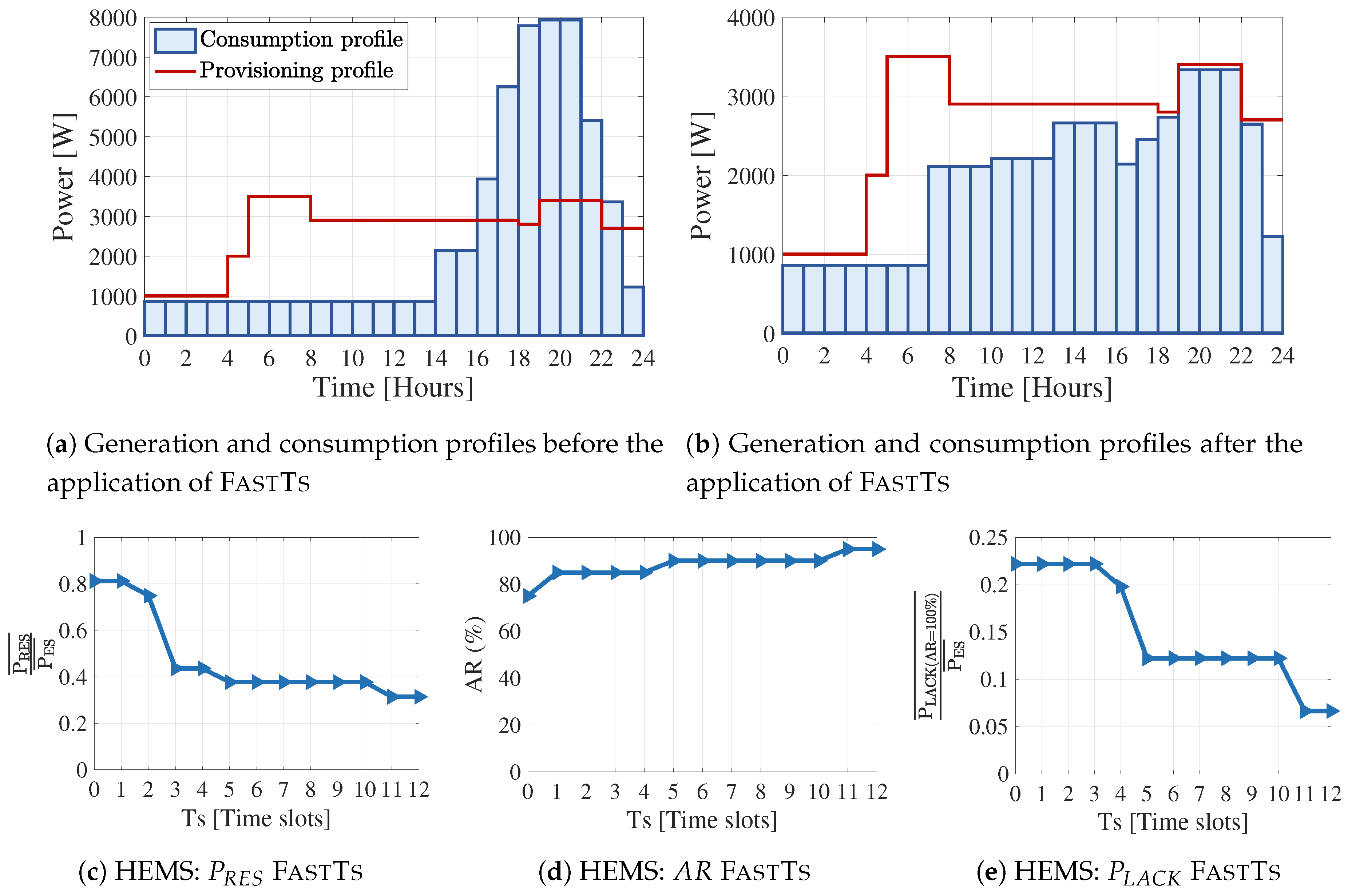
| Case F: HEMS | according to Figure 12a and within m | 0 | 24 | 20 | according to Table 6 | according to Table 6 | according to Table 6 |
| Load Description | Demanded Power [W] | Quantity | l | ||
|---|---|---|---|---|---|
| Freezer | 210 | 1 | 1 | 0 | 24 |
| Refrigerator | 650 | 1 | 1 | 0 | 24 |
| Oven | 1800 | 1 | 3 | 16 | 3 |
| Lighting | 25 | 9 | 1 | 17 | 7 |
| TV | 140 | 1 | 1 | 18 | 5 |
| Laptop | 90 | 1 | 1 | 17 | 5 |
| PC | 140 | 1 | 1 | 18 | 6 |
| Vacuum Cleaner | 600 | 1 | 1 | 19 | 3 |
| Water Heater | 2000 | 1 | 2 | 17 | 6 |
| Air-Conditioner | 1280 | 1 | 2 | 14 | 7 |
| Washing Machine | 1350 | 1 | 3 | 19 | 3 |
| Dishwasher | 1250 | 1 | 3 | 18 | 3 |
| Scenario | No Strategy | OptTs | FastTs | ||
|---|---|---|---|---|---|
| Initial AR | Final AR | AR Gain | Final AR | AR Gain | |
| Case A | 33.33% | 100% | 66.67% | 92.59% | 59.26% |
| Case B | 0% | 100% | 100% | 100% | 100% |
| Case C | 74% | 93% | 19% | 92% | 18% |
| Case D | 67% | 95% | 28% | 94% | 27% |
| Case F | 75% | – | – | 95% | 20% |
| Case A | Case B | Case C | Case D | |||||
|---|---|---|---|---|---|---|---|---|
| Td1 | Td2 | Td3 | Td1 | Td2 | Td3 | |||
| 1 | 0.78 | 0.83 | 1 | 1 | 1 | 0.70 | 0.87 | |
| 1 | 0.78 | 0.83 | 1 | 1 | 1 | 0.73 | 0.97 | |
| 1 | 0.92 | 0.98 | 1 | 1 | 1 | 0.71 | 0.95 | |
| Cases | Running Time OptTs [s] | Running Time FastTs [s] | |
|---|---|---|---|
| Case A | ∼5000× | ||
| Case B | ∼4400× | ||
| Random scenarios, 50 iterations | ∼230× | ||
| Case F | - | - |
| Parameters | AR (%) | (%) | Running Time, 50 Iterations [s] | ||||||
|---|---|---|---|---|---|---|---|---|---|
| N | numPart | No Strategy | FastTs | No Strategy | FastTs | No Strategy | FastTs | FastTs | FastTs |
| 50 | 15 | 0.26 | 0.08 | 0.42 | 0.34 | 59.20 | 74.56 | 15.36 | |
| 20 | 0.09 | 0.35 | 72.72 | 13.52 | |||||
| 25 | 0.10 | 0.36 | 72.66 | 13.46 | |||||
| 100 | 30 | 0.26 | 0.08 | 0.42 | 0.34 | 57.90 | 74.55 | 16.65 | |
| 40 | 0.09 | 0.35 | 73.02 | 15.12 | |||||
| 50 | 0.10 | 0.36 | 72.68 | 14.78 | |||||
| 1000 | 300 | 0.26 | 0.07 | 0.43 | 0.35 | 58.80 | 74.77 | 15.97 | |
| 400 | 0.08 | 0.35 | 73.99 | 15.19 | |||||
| 500 | 0.10 | 0.36 | 72.89 | 14.09 | |||||
| Requirement | Proposed Solution | Comments |
|---|---|---|
| Adaptive consumption constrained to availability |
| The adaptation process must be carried out constantly, and one or all of the proposed management mechanisms can be used for this purpose. |
| Consumer-side participation |
| The participation of the ECs in the energy management process is established through contracts with the ES. These agreements detail all of the technical aspects that are related to the energy demands (e.g., priority) and the possible incentives (e.g., reduce bills) that the ECs can receive by modifying consumption patterns to the availability. |
| Dynamic behavior and scalable computational capacity for adaptive energy management |
| The NFV technology could be deployed on the operations centers available in current smart grids. Additionally, the communications standards, such as SCADA, could migrate to programmable solutions such as SDN. Through these updates, current energy systems could begin their transition to adaptive consumption management. |
| The primary use of renewable energy |
| To ensure energy sustainability, future energy, and communication systems demand the progressive use of green energy sources. Additioonally, the generation from renewable energy sources is a key enabler in the road to a true IoE. In this regard, adaptive energy management solutions are essential to delivering reliable and high-performance energy systems. |
| Adaptive energy management with applicability to small-scale scenarios |
| The optimal solution OptTs is implemented using a brute-force search method and it has an exponential complexity that depends on the maximum values of N and , as shown in Equation (30). Reported limits in the simulation scope are N = 9 services and = 6 time slots. |
| Adaptive energy management with applicability to large-scale scenarios |
| The heuristic solution FastTs is implemented while using a divide-and-conquer approach. The complexity of FastTs in non-linear, but the growth rate is much lower than OptTs. Reported limits on simulation scope are N = 1000 services and = 12 time slots. |
Publisher’s Note: MDPI stays neutral with regard to jurisdictional claims in published maps and institutional affiliations. |
© 2020 by the authors. Licensee MDPI, Basel, Switzerland. This article is an open access article distributed under the terms and conditions of the Creative Commons Attribution (CC BY) license (http://creativecommons.org/licenses/by/4.0/).
Share and Cite
Tipantuña, C.; Hesselbach, X. NFV-Enabled Efficient Renewable and Non-Renewable Energy Management: Requirements and Algorithms. Future Internet 2020, 12, 171. https://doi.org/10.3390/fi12100171
Tipantuña C, Hesselbach X. NFV-Enabled Efficient Renewable and Non-Renewable Energy Management: Requirements and Algorithms. Future Internet. 2020; 12(10):171. https://doi.org/10.3390/fi12100171
Chicago/Turabian StyleTipantuña, Christian, and Xavier Hesselbach. 2020. "NFV-Enabled Efficient Renewable and Non-Renewable Energy Management: Requirements and Algorithms" Future Internet 12, no. 10: 171. https://doi.org/10.3390/fi12100171
APA StyleTipantuña, C., & Hesselbach, X. (2020). NFV-Enabled Efficient Renewable and Non-Renewable Energy Management: Requirements and Algorithms. Future Internet, 12(10), 171. https://doi.org/10.3390/fi12100171