Article

Dynamic Group Recommendation Based on the Attention Mechanism

School of Information Science and Engineering, Shandong Normal University, Jinan 250358, China
*
Author to whom correspondence should be addressed.
Future Internet 2019, 11(9), 198; https://doi.org/10.3390/fi11090198
Submission received: 29 July 2019 / Revised: 7 September 2019 / Accepted: 16 September 2019 / Published: 17 September 2019

Abstract

:
Group recommendation has attracted significant research efforts for its importance in benefiting group members. The purpose of group recommendation is to provide recommendations to group users, such as recommending a movie to several friends. Group recommendation requires that the recommendation should be as satisfactory as possible to each member of the group. Due to the lack of weighting of users in different items, group decision-making cannot be made dynamically. Therefore, in this paper, a dynamic recommendation method based on the attention mechanism is proposed. Firstly, an improved density peak clustering ( DPC ) algorithm is used to discover the potential group; and then the attention mechanism is adopted to learn the influence weight of each user. The normalized discounted cumulative gain (NDCG) and hit ratio (HR) are adopted to evaluate the validity of the recommendation results. Experimental results on the CAMRa2011 dataset show that our method is effective.

1. Introduction

With the rapid development of information technology, the recommendation system has become an important tool for people to solve information overload issues. The recommendation system has been widely used in many online information systems, such as social media sites, E-commerce platforms, etc., to help users choose products [1,2,3] that meet their needs. In addition, the recommendation system is also widely used in medical diagnosis, for example, similar patients may be recommended for similar treatment in one group [4].
Now most of the recommendation systems are designed for individual users, however, group activities have become more and more popular, such as, watching a movie with friends, and planning a trip with other travelers, and having dinner with spouses. Therefore, this requires recommendations for a group of users. Group recommendation [5,6,7] is different from individual recommendation. In a group recommendation, it is used not only to consider the preferences of individual users, but also to consider the preferences of users in the whole group, trying to meet the individual preferences of all members in the group, as much as possible. This requires considering the influence of each member in the group and balancing the preference differences among users. The process is complex and dynamic. For example, a member may play different roles and influences in deciding different types of items due to his/her different expertise. Most of the existing group recommendation methods based on memory and a model adopt predefined group recommendation strategies, which cannot make group decisions dynamically. As a result, the recommendation effect is not ideal.
As a premise of group recommendation, we ask how to discover the potential group, and how to aggregate the preferences of the members of the group to get the results of group recommendation. Specifically, in this work, we propose an improved density peak clustering method to realize group discovery, and use the neural attention network to explore the weight of each user in the group recommendation. By comparing random groups that take the family as the unit, we conclude that the groups with high similarity can be obtained by clustering, and the higher the similarity, the better the group recommendation effect is.
The main work of this paper is summarized as follows:
  • This paper proposes a method for constructing potential groups based on the density peak clustering algorithm. The original density peak clustering algorithm is improved to construct highly similar user sets and realize group division. Improve group recommendation performance.
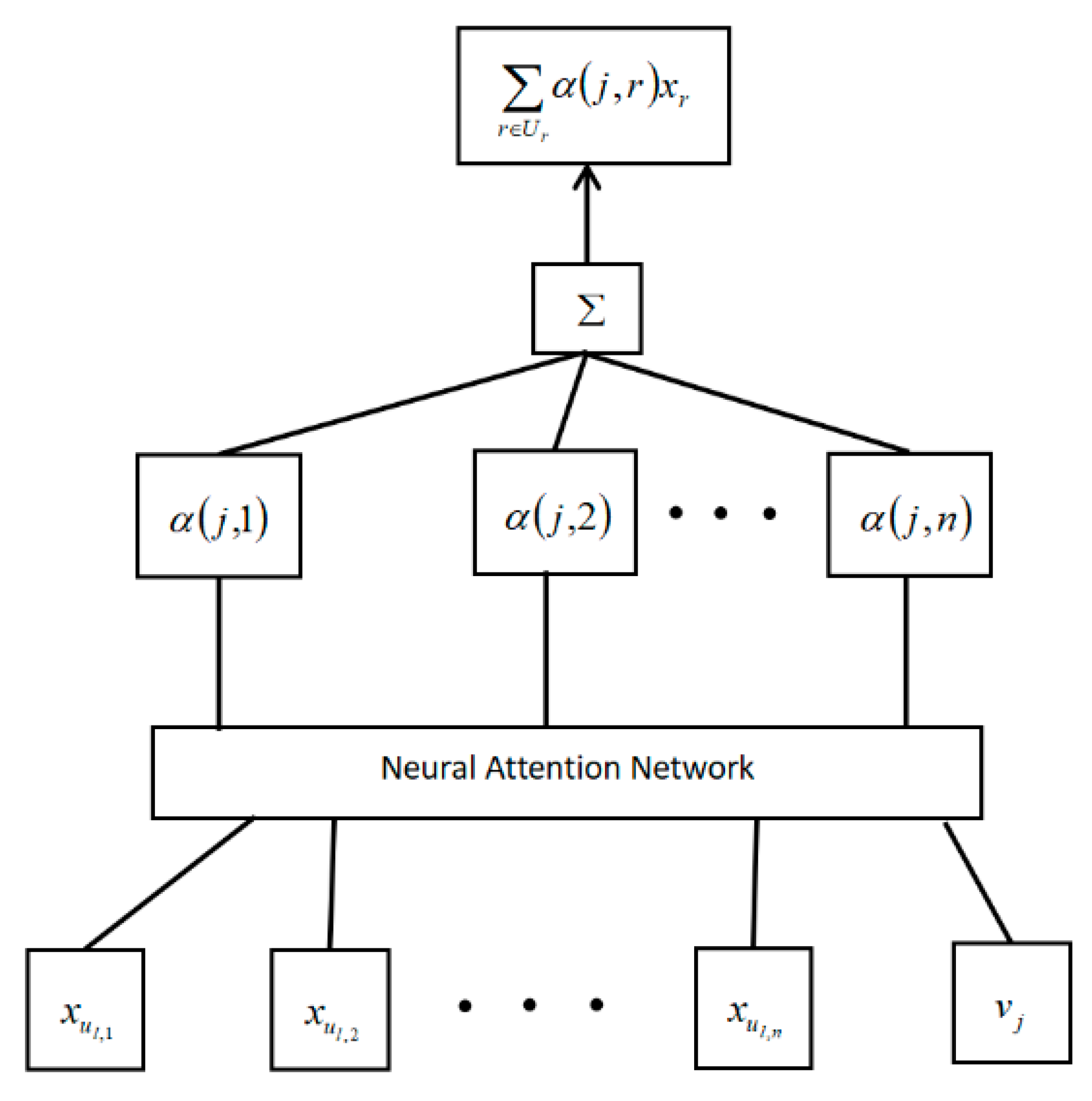
  • Construct the AMGR (attention mechanism group recommended) model and use the neural attention network to dynamically fuse the weight of user preferences within the group to implement group recommendation.
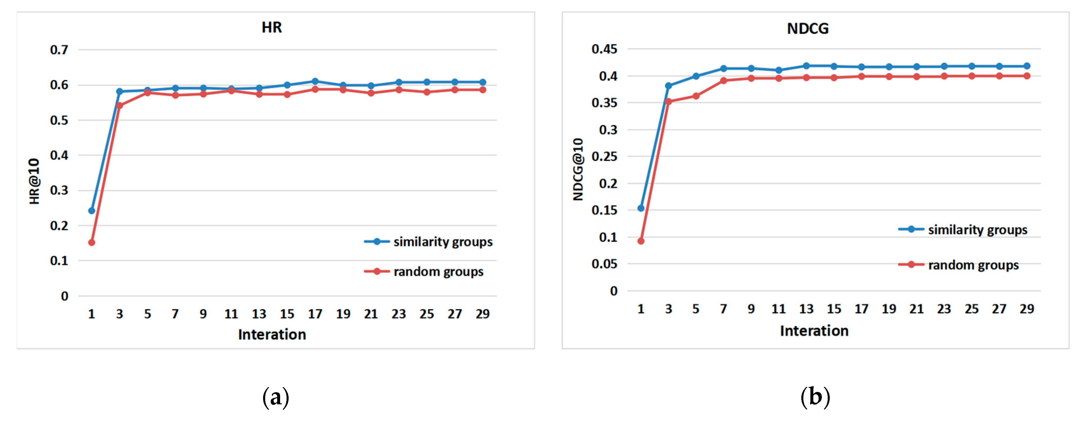
  • We have conducted experiments on a public data set. The experimental results show that the attention network can dynamically capture the overall decision-making process of the group, and the more alike the users in the group are, the better the group recommendation effect will be.

2. Related Work

2.1. Group Division

In group recommendation, since most data sets might not include user group information, or users form groups by random combination, in the research work related to the recommendation system, people propose different user clustering methods according to the user information in the data set. In the work of this paper we attempted to have higher similarity of users together to constitute a group. According to different clustering characteristics, clustering methods can be roughly divided into: Partition-based methods [8,9], hierarchy-based methods [10,11], density-based methods [12,13], grid-based methods [14] and model-based methods [15].
The k-means [16] algorithm is the most commonly used clustering algorithm based on partition. The basic idea is to divide the data into k partitions and then iterative optimize each partition, and divide the samples according to the distance to the cluster represented by the nearest cluster center, and the cluster center is iterative updated. CBoost (cluster-based boosting algorithm) [17], which is an application of the k-means algorithm and uses the k-means algorithm to customize the initial weight value of each data point to deal with the clustering imbalance problem. This algorithm has the advantages of simple and efficient understanding, but the cluster center needs to be selected in advance and only spherical clusters can be found. The validity of the clustering results subject to the selection of the initial cluster center and cluster number.
CURE (clustering using representatives) [18] algorithm is a representative clustering method based on hierarchical decomposition. It does not need to use a single center or object to represent a cluster, but selects a fixed number of representative points in the data space to jointly represent the corresponding cluster, to realize a cluster of arbitrary shape. However, the CURE algorithm has a great impact on the quality of data collection. Hierarchical agglomerative clustering ( HAC ) [19] is a bottom-up clustering algorithm. In the HAC algorithm, each data point is considered as a single cluster, and then the distance between all clusters is calculated to merge the clusters, until all clusters are synthesized into one cluster It has the advantage of being insensitive to the selection of distance metrics, but its efficiency is low.
DBSCAN (density based spatial clustering of applications with noise) [20] is a typical density clustering algorithm, which defines the core object as the data containing the minimum number of data objects MinPts within the neighborhood radius eps, and generates clusters by constantly expanding the data objects reachable with the core object. The DBSCAN algorithm can cluster dense data sets of any shape and is not sensitive to noise data. However, the algorithm has the problems of not being able to reflect the changing density of data sets well, being sensitive to input parameters and has large time cost.
In response to the above problems, many researchers have proposed different solutions. In June 2014, Alex Rodriguez et al. published in Science a new density-based clustering algorithm. The density peak clustering ( DPC ) [21], which can automatically determine the number and center of clusters. The algorithm can quickly find the density peak point (class cluster center) of an arbitrary shape data set. The author thinks that the cluster centers have the characteristics of high local density and larger relative distance with other points with higher density. The DPC algorithm calculates the local density and relative distance of the point, and draws the decision graph (the image with the local density as the X axis and the relative distance as the Y axis). According to the decision graph, the clustering center is manually selected, and then the non-clustering center is merged to achieve the goal of clustering. The DPC algorithm is simple in principle, high in efficiency and suitable for the clustering analysis of large-scale data. However, the algorithm needs to manually set the threshold parameter d c , and the most suitable d c often requires numerous experiments, resulting in low efficiency of the algorithm. In view of this deficiency, this paper improves the selection of the parameter d c of the density peak clustering algorithm.

2.2. Group Recommended

In recent years, the recommendation system has been widely applied to various industries, such as social, e-commerce, medical diagnosis and many studies have been conducted on individual recommendation technology, but research on group recommendation is limited. At present, group recommendation methods can be divided into two categories: Memory-based methods and model-based methods [22,23].
The memory-based methods in group recommendation include the preference aggregation method [24] and score aggregation method [25]. The preference aggregation method is to aggregate the profiles of users in all groups into a new profile, and then perform group recommendations for the user. The score aggregation method calculates the score of each candidate item for each user in the group, and then aggregates the score through a predefined strategy to represent the group’s predictive preference.
Common predefined strategies include the average strategy ( AVG ) [26], the least misery strategy ( LM ) [27], most pleasure strategy ( MP ) [28], etc. AVG first calculates the preference score of each user in the group for each item, and takes the average score as the group preference score. LM selects the lowest of all items scores as the group item recommendation final score. MP selects the highest of all items scores as the final score of group item recommendation. However, these methods are not flexible.
The model-based method is different from the memory-based method. The model-based method first uses the interaction between users in the group to model according to preference information, and then aggregates to generate the preference model of the group. For example, in the personal impact topic model ( PIT ) [29], select the most influential user by considering the influence of the group members, whose decision should represent the group decision. However, this is not the case. Only when the most influential user is an expert in the relevant field, his decision-making is helpful for group recommendation. For example, a food expert may decide which restaurant a group of people go to eat, but may not be the person who decides which movie to go to the theater. The consensus model ( COM ) [30] proposes that the influence of the user depends on the group decision-making theme, and the decision-making process is influenced by two aspects: The group preference topic and the user’s personal preference. The downside of the model at this point is that users cannot dynamically make decisions across groups. In addition, there is a recommendation algorithm based on matrix factorization ( MF ) [31] methods. MF is the decomposition of a matrix into the product of two or more matrices, in which the most basic data is the user–item scoring matrix, and the missing score can be converted into a regression problem based on machine learning. The advantage of this method is that the prediction accuracy is high, but the model training is time-consuming and does not have a good interpretation.
In recent years, deep learning has been widely applied to the recommendation system by the research community, which combines the deep learning method with the recommendation system to capture various relationships between users and item. The literature [32,33] has a comprehensive review. However, there are relatively few researches on group recommendation using deep learning. In this paper, we used the neural network and attention mechanism to dynamically learn the weights of users in the group and make group recommendations. The specific details will be shown below.

3. Methods

In this section, we will introduce the use of the improved density peak algorithm to construct a group with higher similarity, and then introduce our AMGR model to implement a group recommendation.

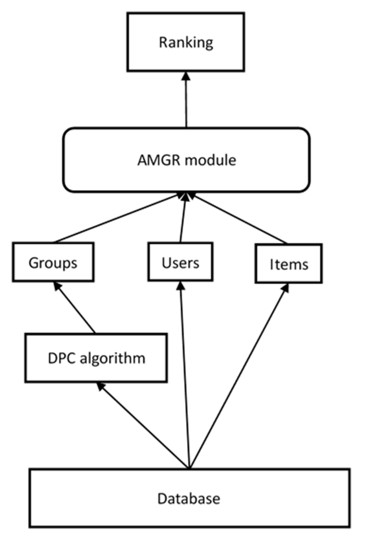
3.1. Overview of the Group Recommended

Our goal was to recommend the item to a group of users, and the result of the recommendation was to maximize the satisfaction of all users in the group. As shown in Figure 1. Firstly, we used the improved density peak clustering algorithm to aggregate users with high similarity and discover potential groups. Then group recommendation was implemented using the AMGR model we built. The AMGR model consists of two components: Fusion group preference and interactive learning to use the NCF (neural collaborative filtering) [34] framework.

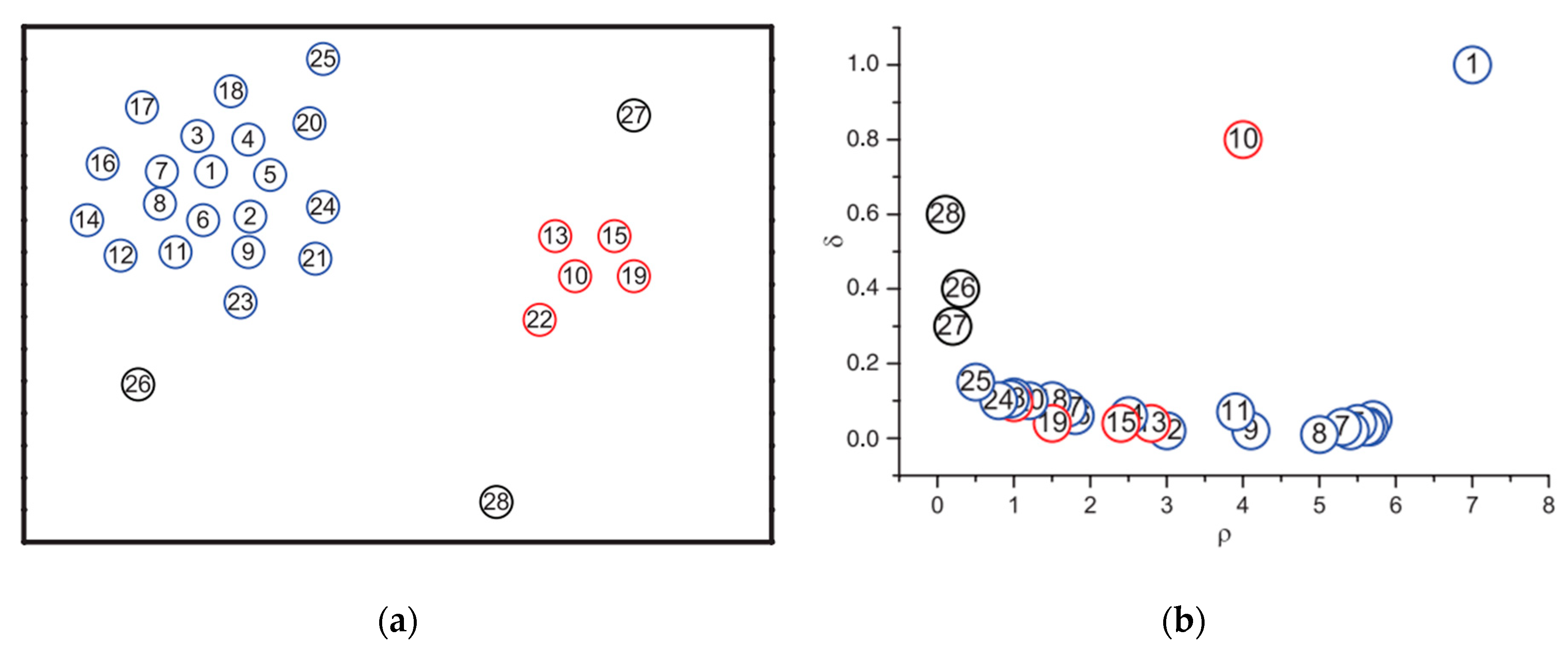
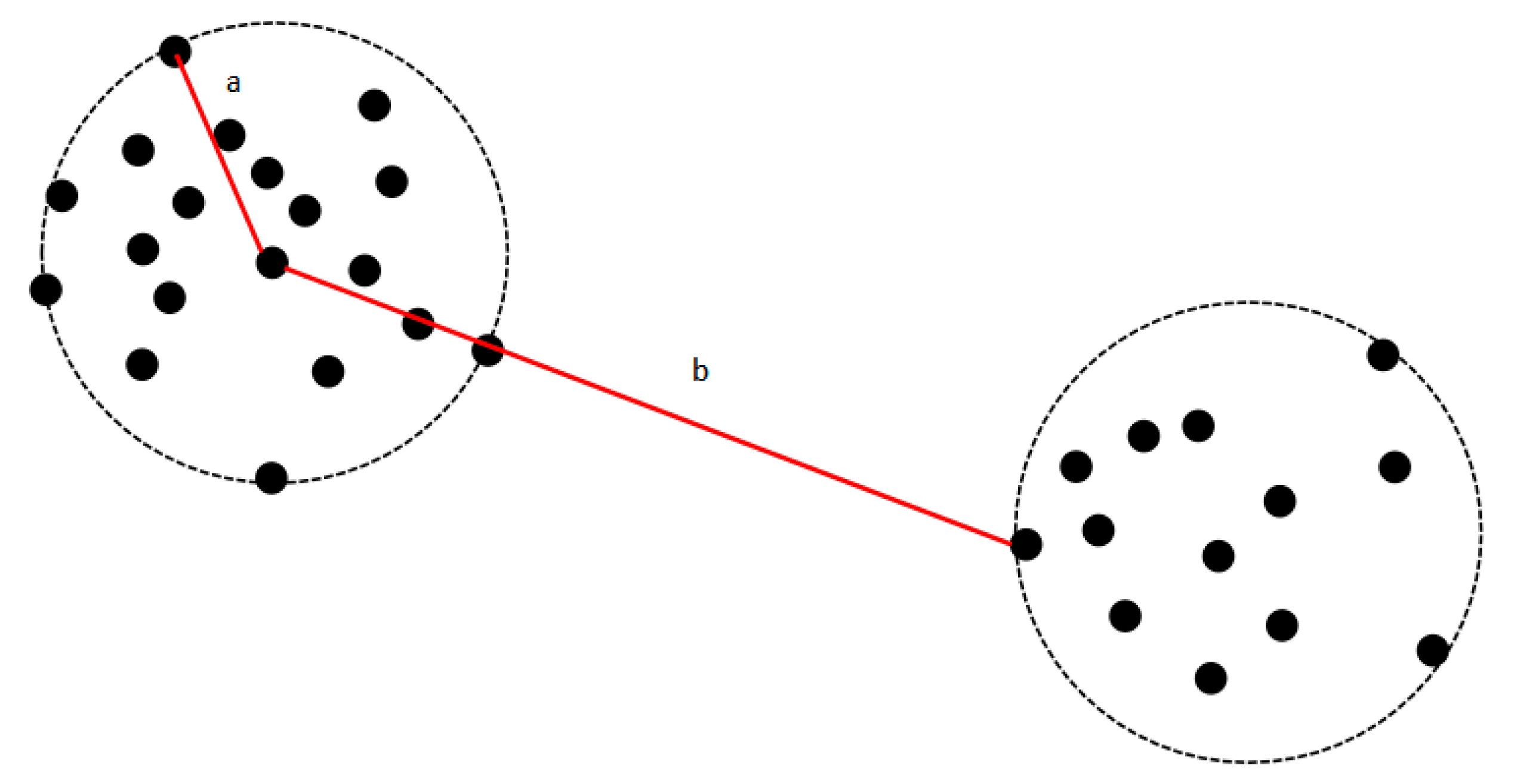
3.2. Density Peak Clustering Algorithm

The idea of the DPC algorithm is to represent the distance of a certain number of points based on the local density. The more points around a point, the larger the local density. The clustering center has the following two characteristics: (1) The local density of data points is relatively large, which is surrounded by some data objects with low local density and (2) the points with high local density are relatively far away from other points with high local density. The local density and relative distance of the algorithm use ρ i and δ i to represent these two features, respectively, and the clustering center is to select the point where ρ i and δ i are relatively large. The processing flow of DPC algorithm can be summarized as the following steps: (1) Setting the cutoff distance d c , calculate the local density ρ i and high-density distance δ i according to the set d c distance value, and marking the point that has a higher density than each other point. (2) The density peak needs to be found in the decision graph, i.e., the clustering center. (3) Assign the remaining data points to the class where the density is higher than itself and the nearest point is located.
For the local density ρ i of the data object x i , there are two calculation methods: Cut-off kernel and Gaussian kernel.
Cut-off kernel is defined as:
ρ i = j χ ( d i j d c ) ,
where d i j represents the certain distance between data points x i and x j and d c is a preset value, which indicates that the cutoff distance ( d c > 0 ) . Generally, the first 2% of the distance between two data objects in ascending order is regarded as the cutoff distance and the χ () function is defined as follows:
χ ( x ) = { 1   ,   x < 0 0   ,   x 0 .
Gaussian kernel is defined as:
ρ i = j e ( d i j d c ) 2 .
The difference between the cut-off kernel and Gaussian kernel is that the cut-off kernel results are discrete values while Gaussian kernel results are continuous values. Relatively speaking, the conflicts generated by the latter (that is, different data points have the same local density) are less probable. Literature [35] adopted the cut-off kernel and Gaussian kernel local density calculation methods for classical data set path-based2 respectively, which proves that the DPC algorithm adopted Equation (3), Gaussian kernel, to measure the local density clustering effect better.
For the relative distance of data point x i , there are the following calculation methods:
δ i = m i n j : ρ j > ρ i ( d i j ) .
From Equation (4), δ i indicates the relative distance, that is, for each data point x i , finds all data points x j , which are denser than the data point x i , and selects the smallest d i j as δ i . If data point x i is the highest local density data point, δ i is defined as δ i = m a x j ( d i j ) , which is the maximum distance from all data points to data point x i .
The decision graph is an innovation in the DPC algorithm. For each data point x i in the data set, it needs to calculate the local density ρ i and relative distance δ i separately, Then, according to the calculated values, each data point is in the form of a binary pair ( ρ i , δ i ) , and a two-dimensional planar decision diagram is drawn (with ρ i as the horizontal axis and δ i as the vertical axis). Figure 2 is a distribution with 28 two-dimensional data points, and the data points are arranged in descending order of density.
As can be seen from Figure 2b, numbers 1 and 10 stands out because they have both larger values of ρ and δ , which are the two clustering centers in the data set of Figure 2a. The numbering number 26, number 27 and number 28 is characterized by a small value of ρ , but a large value of δ , which is called an outlier.

3.3. Improvement

This algorithm needs to solve two problems: (1) The distance d i j between different nodes needs to be calculated. In this paper, the similarity between users is taken as the distance between nodes. The similarity distance between user i and user j is based on the score of the same item that is determined, and the similarity is calculated as follows:
d i j = 1 | M |   m M s m i s m j ,
where d i j represents the difference distance between user i and user j , s m i indicating the score of user i for item m , similarly s m j indicating the score of user j for item m , the set of items graded by both user i and user j is represented by M and | M | denotes the number of elements in the set. The greater the difference between the two users, the farther the distance.
(2) The calculation of local density ρ i and distance δ i in DPC depends on the cutoff distance d c . The selection of d c is based on a manual setting, and the optimal d c usually needs the experimenter to obtain through many experiments. Whether d c selection is appropriate or not has a certain influence on the DPC algorithm. If d c is too large, all data points will be classified into one class in extreme cases, on the other hand, if d c is too small, all data points become a single class in extreme cases. Since d c selection is particularly important, in this paper, the d c to select has made the improvement.
The vector: c i = { d i 1 , d i 2 , , d i n } where d i j is the distance between user i and user j , i.e., similarity, and sorts them in ascending order to get the vector f i = { a i 1 , a i 2 , , a i n } , then the cutoff distance of user i can be defined as:
d c i = a i j | m a x ( a i ( j + 1 ) a i j ) .
According to Equation (6), the cutoff distance d c i of user i is taken as the maximum value of the difference between two elements of vector f i . Obviously, the distance difference between users belonging to the same cluster is relatively small, whereas the distance difference between users in different clusters is relatively large, as shown in Figure 3.
Select the a i j with the largest difference between the two adjacent elements in f i , where a i j = a , a i ( j + 1 ) = b and d c i = a i j | m a x ( a i ( j + 1 ) a i j ) = a .
The equation is still applicable when a i ( j + 1 ) is an outlier. The set D c = { d c 1 , d c 2 , , d c n } represents the set of d c i corresponding to each user i . In order to reduce the influence of the points on the cluster boundary and the outliers and avoid excessive d c , d c should take the minimum value of the set D c , ρ i and δ i should be calculated according to the Equations (1) or (3) and (4), after d c is determined.
This method of determining d c is based on the distance between data objects, so it does not add extra calculation burden and is simple and easy to implement.

3.4. Group Recommendation Method

3.4.1. Problem Formulation

In this paper, we used uppercase letters and lowercase letters to represent the matrix and vector respectively, and the set was represented by skewed letters. Let X = { x 1 , x 2 , , x n } , V = { v 1 , v 2 , , v w } and G = { g 1 , g 2 , , g e } be the sets of n users, w items and e groups, respectively. g l represents the l -th specific group ( g l G ), and the user who constitutes g l is expressed as U l = { u l 1 , u l 2 , , u l r , } , r is the size of the group g l , Q = [ q l j ] e × w and S = [ s i j ] n × w represents the group–item interaction matrix and the user–item interaction matrix.
Input: X , V , G , Q , S .
Output: Give scores about an item for each group and each user by two personalized ranking functions.

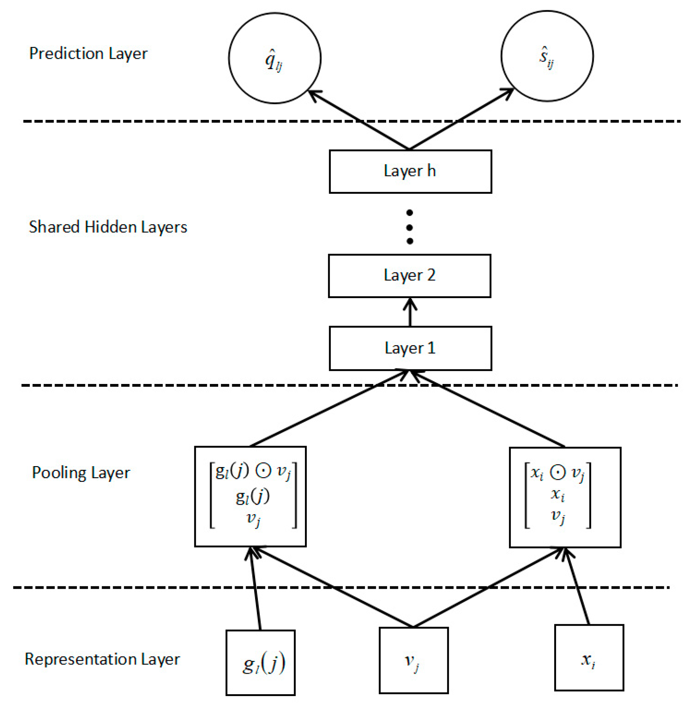
3.4.2. Attention Mechanism Model

In recent years, the attention mechanism has been successfully applied to a variety of machine learning tasks. Attention is that when people see an object, they tend to focus on the important parts of the object rather than the whole of the object. Inspired by this, we recommended that we use the neural attention mechanism [36], which can learn aggregation strategy for groups. The main idea was to learn the weight of a user relative to other users in the group as a whole. The weights were learned in neural networks. The weight was learned by the neural network. The higher the user weight, the more important the user’s decision is.
In the representation learning (RL) paradigm, we represent each entity as an embedded vector, which encodes the attributes of the entity, such as user gender, hobbies, etc. Let user x i and v j represent the embedding vectors of user x i and item v j , and group embedding is defined as:
g l ( j ) = f a ( v j , { x r } r U l ) ,
The embedding of the group depends on the embedding of its user members and target items, where g l ( j ) represents the preference prediction of the embedded group g l for the item v j , f a is the specified aggregate function, which can be further expressed as:
f a = r U l α ( j , r ) x r ,
For item v j , the weight parameter α ( j , r ) is defined to represent the weight corresponding to item embedding of the group depends on the embedding of its user members and target items v j and user x r . That is to say, if the user has more professional knowledge about an item or similar item, then he has greater influence on the selection of the item in the group, and the weight is greater. The calculation method is as follows:
o ( j , r ) = h T R e L U ( p v v j + p u x r + b ) ,
α ( j , r ) = s o f t m a x ( o ( j , r ) ) = e x p o ( j , r ) r U l e x p o ( j , r ) ,
The user embedding vector the x r , the target item embedding vector v j as the input of the neural attention network, the weight matrix of the attention network is expressed by p v , p u , b , as the bias vector, It is activated by the Rectifier Linear Unit ( R e L U ) [37] function, and then item to the weight vector h . Finally, the score o ( j , r ) is normalized by softmax [38]. The process is shown in Figure 4.

3.4.3. Predicted Score

Our goal is to achieve both individual recommendation and group recommendation. Since the neural network has strong data fitting ability, NCF framework is used. Its basic idea is to feed embed users and items into the dedicated neural network to learn interactive functions. Figure 5 is a sketch of NCF framework.
Specifically, given a group–item pair or user–item pair, returning the corresponding embedding vector to each entity in the presentation layer (the specific method is 3.4.2). Suppose the group–item pair we input, the pooling layer performs the element connection, where corresponds to element-wise multiplication i.e.,:
z 0 = Φ p o o l i n g ( g l ( j ) , v j ) = [ g l ( j ) v j g l ( j ) v j ] ,
Since group embedding is obtained by user embedding aggregation, they are in the same semantic space, so it is a shared hidden layer on the pooling layer, capturing non-linearity and high-order correlation among users, groups and items.
{ z 1 = R e L U ( W 1 z 0 + b 1 ) z 2 = R e L U ( W 2 z 1 + b 2 ) z h = R e L U ( W h z h 1 + b h ) ,
W h , b h , and z h represent the weight matrix, bias vectors and output neurons of the hidden layer of layer respectively. They are activated by R e L U function. Finally, the last layer z h is output to calculate the prediction score:
{ q ^ l j = W T z h ,   i f   z 0 = Φ ( g l ( j ) , v j ) s ^ i j = W T z h ,   i f   z 0 = Φ ( x i , v j ) ,
W represents the weight of the prediction layer, q ^ l j and s ^ i j respectively represent the prediction scores of the group–item pair and user–item pair, respectively.

3.4.4. Objective Function

We used pairwise learning to optimize model parameters, assuming that the predictive scores of observable interactive items were higher than those of the unobserved, here we used regression-based pairwise loss [39]:
u s e r = ( i , j , p O ) ( s i j p s ^ i j p ) 2 = ( i , j , p O ) ( s ^ i j s ^ i p 1 ) 2 ,
s ^ i j p = s ^ i j s ^ i p ,
where s i j p = s i j s i p , definition ( i , j , p ) is an instance (triplet) in training set O , which indicates that interaction relation can be observed between user x i and item v j but no interaction relation is observed with item v p ( v j is a positive instance and v p is a negative instance). The value of the interaction relation can be observed to be 1 (that is, s i j = 1 ), and the value of the interaction relation not observed to be 0 (that is, s i p = 0 ). From Equation (15) s ^ i j p represents the predicted margin between the observable ( x i , v j ) and the observable ( x i , v p ) .
Similarly, pairwise loss functions are recommended for the group:
g r o u p = ( l , j , p O ) ( q l j p q ^ l j p ) 2 = ( l , j , p O ) ( q ^ l j q ^ l p 1 ) 2 .
In training set O , group l has an interactive relationship with item v j , but not with item v p .
We realized that another popular pairwise learning method could also be applied in the recommendation, such as Bayesian personalized ranking (BPR), etc. In this paper, we adopted regression-based ranking loss and we will explore other methods in future work.

4. Experiments and Analysis

In this section, we conducted experiments on the CAMRa2011 data set and answered the following questions:
RQ1: How effective are the recommendations caused by two different organizational groups?
RQ2: How does our attention model method compare with other methods?

4.1. Experimental Settings

4.1.1. Dataset

The experiment in this section used CAMRa2011, a data set, which included individual users’ scoring records for movies and group scoring records for movies. The composition of the group was based on the family, and the family members had a greater preference. Since there were some users in the data set who did not join the group, we chose to filter out the users who only retained the group information. The rating was between 0 and 100. We changed the rate of the record as a positive instance with a target value of 1 and other lost data were kept as a negative instance of the target the value, which was 0. Finally, the data set we used was filtered from the original data set. The data set included 602 users, 290 groups, 7710 movies, 116,344 interactive records of user items and 145,068 interactive records of group items, respectively.
Now there were only positive instances in the data set, that is, interactive relationships could be observed. For negative instances, we randomly sampled the missing data as negative instances and paired them with positive instances. In the previous related work, we learned that when the negative sample was increased from 1 to a certain value, this was beneficial for the top-k recommendation. Therefore, for the data set used in the experiment, we selected the negative sample ratio as 4, randomly selected the four movies with no interactive relationship (never seen) and assigned a value of 0 to each negative instance.

4.1.2. Evaluation

We used protocol leave-one-out, which is widely used to evaluate top-k recommendation performance, to separate the training set from the test set. Specifically, for each user or group, we randomly deleted one of its interactions for testing. In our experiment, we randomly selected 100 items without user or group interaction, and ranked the test items in these 100 items. We used two indicators—hit ratio ( HR ) and normalized discount cumulative gain ( NDCG ) .
HR is a commonly used indicator for calculating the balance recall rate in the top-k recommendation. The calculation equation is:
HR @ K = N u m b e r   o f   Hit @ K GT .
The denominator GT is the set of all tests, while the numerator represents the sum of the number of test sets belonging to each user’s top-K list.
NDCG is used to evaluate the accuracy of the top-K recommendation list. The calculation equation is:
NDCG @ K = DCG IDCG ,
DCG = i = 1 k 2 r e l i 1 l o g 2 ( i + 1 ) ,
where r e l i represents the relevance of the recommendation result for location i , while k stands for the size of the recommendation list. IDCG represents a list of the best recommended results returned by a user of the recommendation system ( IDCG stands for DCG in order of rating). Use IDCG for normalization to get NDCG , the value of NDCG is between 0 and 1. The closer the result is to 1, the better the recommendation effect.

4.1.3. Baselines

In the experiment we compared the following methods.
Popularity: It is a non-personalized recommendation method that recommends items to users and groups based on the popularity of the product. Popularity is measured by the number of interactions of an item in a training set.
COM: This is a process probability model used to simulate group recommendation. The group’s preferences for an item are estimated by aggregating the preferences of the members of the group.
AVG (NCF): Firstly, the NCF method is used to predict the preference score of the members in the group. Each member in the group contributes equally to the group decision-making, and the average score is taken as the group preference score.
LM (NCF): The NCF method was used to predict the preference score of members in the group, and the lowest score was used as the preference score of the group.
MP (NCF): Similarly, the NCF method was used to predict the preference score of members in the group, and the highest score was used as the preference score of the group.
MGR: In order to prove the recommendation effect of group members with different weights, we used MGR , which removes the attention model to assign unified weights to users.

4.1.4. Parameter Setting

Our method was based on pytorch implementation. Since Glorot initialization strategy has good performance, we used the Glorot initialization strategy in the initialization setting of embedded layers. We used Gaussian distribution to initialize the hidden layer. The average value was 0 and the standard deviation was 0.1. Gradient-based methods all use the Adam optimizer, which the minibatch size searched in 128, 256, 512, 1024 and learning rate 0.001, 0.005, 0.01, 0.05, 0.1. In NCF , we set the size of the first hidden layer to be 32 and the size of the embedded layer to be the same, using a three-layer tower structure and a ReLU activation function. We repeated each setup five times and reported the average results.

4.2. Effect of Group Recommendations (RQ1)

In this experiment, we proposed a clustering method based on peak density to construct groups with high similarity for users in random groups (taking family as a unit, user similarity difference is large). Group recommendation methods based on the attention mechanism were respectively applied to them. In fact, our intuition also told us that the less similar the user is, the worse the group recommendation will be. Since it is difficult to find a consensus among different preferences to satisfy the users in the group. Figure 6 shows the results of our experiments with random group and highly similar group. We used two indicators, HR and NDCG , to report average results based on five experimental results.
Figure 6a,b shows the performance of iterative training for highly similar groups and random groups under optimal parameters respectively. The blue line represents high similarity groups and the red line represents random groups. We note that compared with the random group, the high similarity group made certain progress in both indicators, and its performance tended to be stable after 15 iterations. We verified our view through this experiment. The higher the overall similarity of the group users, the more satisfied they were with the items recommended by the group, and the better the group recommendation performance.

4.3. Overall Performance Comparison (RQ2)

In this section, we compared the AMGR model with the baselines. Table 1 shows the values of HR and NDCG in different methods at k = 5. Table 2 shows the values of HR and NDCG in different methods at k = 10.
Now we compared the performance of the AMGR model with the above methods. Note that the COM model is the group recommendation and cannot be recommended for a single user, so the table data is empty. From Table 1 and Table 2, it can be seen that the method based on NCF was better than the COM model and the popularity model because of the superiority of the neural network. In addition, when k = {5,10} of our model, HR and NDCG were higher than other models, which verified that the AMGR model was superior to the above method. Specifically, the attention network we used dynamically allocated the weight of members in the group and aggregated preferences according to different items, which could effectively achieve user recommendation and group recommendation, and the model recommendation effect had certain advantages.

5. Conclusions and Future Work

In this work, we constructed the AMGR model. Specifically, we dynamically learnt the user preference weights in the group through the attention network. Then, we used the NCF framework to learn the complex interaction data between user–item and group–item to achieve a group recommendation. In addition, we analyzed the group recommendation performance between random groups and highly similar groups. We suggest using the improved density peak clustering method to aggregate users with high similarity to form a high similarity group, and then make a group recommendation. In order to verify the effectiveness of group recommendation, we conducted experiments on a data set, and the results showed that our model had a better recommendation effect, and also verified that the more similar users in the group were, the better the group recommendation effect was.
In future work, we will improve the inadequacy of this work (small errors may exist in the objective function). Since the users’ preferences will change with different times and places, we will also take into account the time and location, which will further improve the effectiveness of the group recommendation system.

Author Contributions

Y.D. obtained funding; H.X. proposed the topic and implemented the framework. H.X. wrote the paper. J.S., K.Z., Y.C., and Y.D. improved the quality of the manuscript.

Funding

Primary Research & Development Plan of Shandong Province (2017GGX10112).

Acknowledgments

Thanks to all commenters for their valuable and constructive comments.

Conflicts of Interest

The authors declare no conflict of interest.

References

  1. Yang, Z.; Wu, B.; Zheng, K.; Wang, X.; Lei, L. A survey of collaborative filtering-based recommender systems for mobile Internet applications. IEEE Access 2016, 4, 3273–3287. [Google Scholar] [CrossRef]
  2. Wei, J.; He, J.; Chen, K.; Zhou, Y.; Tang, Z. Collaborative filtering and deep learning based recommendation system for cold start items. Expert Syst. Appl. 2017, 69, 29–39. [Google Scholar] [CrossRef]
  3. Balakrishnan, J.; Cheng, C.H.; Wong, K.F.; Woo, K.H. Product recommendation algorithms in the age of omnichannel retailing—An intuitive clustering approach. Comput. Ind. Eng. 2018, 115, 459–470. [Google Scholar] [CrossRef]
  4. Thanh, N.D.; Ali, M. A novel clustering algorithm in a neutrosophic recommender system for medical diagnosis. Cogn. Comput. 2017, 9, 526–544. [Google Scholar] [CrossRef]
  5. Kim, J.K.; Kim, H.K.; Oh, H.Y.; Ryu, Y.U. A group recommendation system for online communities. Int. J. Inf. Manag. 2010, 30, 212–219. [Google Scholar] [CrossRef]
  6. Cao, D.; He, X.; Miao, L.; An, Y.; Yang, C.; Hong, R. Attentive group recommendation. In Proceedings of the 41st International ACM SIGIR Conference on Research & Development in Information Retrieval, Ann Arbor, MI, USA, 8–12 July 2018; pp. 645–654. [Google Scholar]
  7. Xia, B.; Li, Y.; Li, Q.; Li, T. Attention-based recurrent neural network for location recommendation. In Proceedings of the 12th International Conference on Intelligent Systems and Knowledge Engineering (ISKE), Nanjing, China, 24–26 November 2017; pp. 1–6. [Google Scholar]
  8. Boley, D.; Gini, M.; Gross, R.; Han, E.-H.S.; Hastings, K.; Karypis, G.; Kumar, V.; Mobasher, B.; Moore, J. Partitioning-based clustering for web document categorization. Decis. Support Syst. 1999, 27, 329–341. [Google Scholar] [CrossRef]
  9. Zhang, Y.; Xiong, Z.; Mao, J.; Ou, L. The study of parallel k-means algorithm. In Proceedings of the 6th World Congress on Intelligent Control and Automation, Dalian, China, 21–23 June 2006; pp. 5868–5871. [Google Scholar]
  10. Mirzaei, A.; Rahmati, M. A novel hierarchical-clustering-combination scheme based on fuzzy-similarity relations. IEEE Trans. Fuzzy Syst. 2009, 18, 27–39. [Google Scholar] [CrossRef]
  11. Handy, M.; Haase, M.; Timmermann, D. Low energy adaptive clustering hierarchy with deterministic cluster-head selection. In Proceedings of the 4th International Workshop on Mobile and Wireless Communications Network, Stockholm, Sweden, 9–11 September 2002; pp. 368–372. [Google Scholar]
  12. Wang, X.F.; Huang, D.S. A novel density-based clustering framework by using level set method. IEEE Trans. Knowl. Data Eng. 2009, 21, 1515–1531. [Google Scholar] [CrossRef]
  13. Kriegel, H.P.; Kröger, P.; Sander, J.; Zimek, A. Density-based clustering. Wiley Interdiscip. Rev. Data Min. Knowl. Discov. 2011, 1, 231–240. [Google Scholar] [CrossRef]
  14. Grabusts, P.; Borisov, A. Using grid-clustering methods in data classification. In Proceedings of the International Conference on Parallel Computing in Electrical Engineering, Warsaw, Poland, 22–25 September 2002; pp. 425–426. [Google Scholar]
  15. Mann, A.K.; Kaur, N. Survey paper on clustering techniques. Int. J. Sci. Eng. Technol. Res. 2013, 2, 803–806. [Google Scholar]
  16. Kanungo, T.; Mount, D.M.; Netanyahu, N.S.; Piatko, C.D.; Silverman, R.; Wu, A.Y. An efficient k-means clustering algorithm: Analysis and implementation. IEEE Trans. Pattern Anal. Mach. Intell. 2002, 7, 881–892. [Google Scholar] [CrossRef]
  17. Le, T.; Le Son, H.; Vo, M.; Lee, M.; Baik, S. A cluster-based boosting algorithm for bankruptcy prediction in a highly imbalanced dataset. Symmetry 2018, 10, 250. [Google Scholar] [CrossRef]
  18. Naresh, V.R.K.; Gope, D.; Lipasti, M.H. The CURE: Cluster Communication Using Registers. ACM Trans. Embed. Comput. Syst. 2017, 16, 124. [Google Scholar] [CrossRef]
  19. Müllner, D. Fastcluster: Fast hierarchical, agglomerative clustering routines for R and Python. J. Stat. Softw. 2013, 53, 1–18. [Google Scholar] [CrossRef]
  20. Bryant, A.; Cios, K. RNN-DBSCAN: A density-based clustering algorithm using reverse nearest neighbor density estimates. IEEE Trans. Knowl. Data Eng. 2018, 30, 1109–1121. [Google Scholar] [CrossRef]
  21. Rodriguez, A.; Laio, A. Clustering by fast search and find of density peaks. Science 2014, 344, 1492–1496. [Google Scholar] [CrossRef] [PubMed] [Green Version]
  22. Koren, Y.; Bell, R.; Volinsky, C. Matrix factorization techniques for recommender systems. Computer 2009, 8, 30–37. [Google Scholar] [CrossRef]
  23. Su, X.; Khoshgoftaar, T.M. A survey of collaborative filtering techniques. Adv. Artif. Intell. 2009, 2009, 421425. [Google Scholar] [CrossRef]
  24. Baskin, J.P.; Krishnamurthi, S. Preference aggregation in group recommender systems for committee decision-making. In Proceedings of the Third ACM Conference on Recommender Systems, New York, NY, USA, 22–25 October 2009; pp. 337–340. [Google Scholar]
  25. Baltrunas, L.; Makcinskas, T.; Ricci, F. Group recommendations with rank aggregation and collaborative filtering. In Proceedings of the Fourth ACM Conference on Recommender Systems, Barcelona, Spain, 26–30 September 2010. [Google Scholar]
  26. Berkovsky, S.; Freyne, J. Group-based recipe recommendations: Analysis of data aggregation strategies. In Proceedings of the Fourth ACM Conference on Recommender Systems, Barcelona, Spain, 26–30 September 2010; pp. 111–118. [Google Scholar]
  27. Amer-Yahia, S.; Roy, S.B.; Chawlat, A.; Das, G.; Yu, C. Group recommendation: Semantics and efficiency. Proc. VLDB Endow. 2009, 2, 754–765. [Google Scholar] [CrossRef]
  28. Boratto, L.; Carta, S. State-of-the-art in group recommendation and new approaches for automatic identification of groups. In Information Retrieval and Mining in Distributed Environments; Springer: Berlin/Heidelberg, Germany, 2010; pp. 1–20. [Google Scholar]
  29. Liu, X.; Tian, Y.; Ye, M.; Lee, W.C. Exploring personal impact for group recommendation. In Proceedings of the 21st ACM International Conference on Information and Knowledge Management, Maui, HI, USA, 29 October–2 November 2012; pp. 674–683. [Google Scholar]
  30. Yuan, Q.; Cong, G.; Lin, C.Y. COM: A generative model for group recommendation. In Proceedings of the 20th ACM SIGKDD International Conference on Knowledge Discovery and Data Mining, New York, NY, USA, 24–28 August 2014; pp. 163–172. [Google Scholar]
  31. Ma, H.; Yang, H.; Lyu, M.R.; King, I. Sorec: Social recommendation using probabilistic matrix factorization. In Proceedings of the 17th ACM Conference on Information and Knowledge Management, Napa Valley, CA, USA, 26–30 October 2008; pp. 931–940. [Google Scholar]
  32. Karatzoglou, A.; Hidasi, B. Deep learning for recommender systems. In Proceedings of the Eleventh ACM Conference on Recommender Systems, Como, Italy, 23–31 August 2017; pp. 396–397. [Google Scholar]
  33. Zhang, S.; Yao, L.; Sun, A.; Tay, Y. Deep learning based recommender system: A survey and new perspectives. ACM Comput. Surv. 2019, 52, 5. [Google Scholar] [CrossRef]
  34. He, X.; Liao, L.; Zhang, H.; Nie, L.; Hu, X.; Chua, T.S. Neural collaborative filtering. In Proceedings of the 26th International Conference on World Wide Web, International World Wide Web, Perth, Australia, 3–7 April 2017; pp. 173–182. [Google Scholar]
  35. Chang, H.; Yeung, D.Y. Robust path-based spectral clustering. Pattern Recog. 2008, 4, 191–203. [Google Scholar] [CrossRef]
  36. Xiao, J.; Ye, H.; He, X.; Zhang, H.; Wu, F.; Chua, T.S. Attentional factorization machines: Learning the weight of feature interactions via attention networks. arXiv 2017, arXiv:1708.04617. [Google Scholar]
  37. Krizhevsky, A.; Sutskever, I.; Hinton, G.E. Imagenet classification with deep convolutional neural networks. In Proceedings of the Advances in Neural Information Processing Systems, Lake Tahoe, NE, USA, 3–6 December 2012; pp. 1097–1105. [Google Scholar]
  38. Chen, J.; Zhang, H.; He, X.; Nie, L.; Liu, W.; Chua, T.-S. Attentive collaborative filtering: Multimedia recommendation with item-and component-level attention. In Proceedings of the 40th International ACM SIGIR Conference on Research and Development in Information Retrieval, Tokyo, Japan, 7–11 August 2017; pp. 335–344. [Google Scholar]
  39. Wang, X.; He, X.; Nie, L.; Chua, T.S. Item silk road: Recommending items from information domains to social users. In Proceedings of the 40th International ACM SIGIR Conference on Research and Development in Information Retrieval, Tokyo, Japan, 7–11 August 2017; pp. 185–194. [Google Scholar]
Figure 1. Overview of the group recommended.
Futureinternet 11 00198 g001
Figure 2. (a) Data point distribution and (b) decision diagram.
Futureinternet 11 00198 g002
Figure 3. Cutoff distance.
Futureinternet 11 00198 g003
Figure 4. User embedding aggregation based on neural attention.
Futureinternet 11 00198 g004
Figure 5. Neural   collaborative   filtering   ( NCF ) interactive learning.
Futureinternet 11 00198 g005
Figure 6. (a) Effectiveness of group recommendation ( HR @ 10 ) and (b) the effectiveness of group recommendation ( NDCG @ 10 ) .
Futureinternet 11 00198 g006
Table 1. Performance comparison baseline at k = 5. Best results are in bold.
MethodsUserGroup
HR@5NDCG@5HR@5NDCG@5
Popularity0.37250.26540.34940.2375
COM--0.48900.3310
AVG (NCF)--0.47930.3365
LM (NCF)--0.47030.3335
MP (NCF)--0.45640.3257
MGR0.50470.37620.49810.3419
AMGR0.52180.38030.49930.3502
Table 2. Performance comparison baseline at k = 10. Best results are in bold.
MethodsUserGroup
HR@10NDCG@10HR@10NDCG@10
Popularity0.42460.23380.40130.2079
COM--0.58980.3957
AVG (NCF)--0.58960.3994
LM (NCF)--0.59070.4061
MP (NCF)--0.58960.3943
MGR0.61030.41620.59080.4019
AMGR0.62620.42430.60760.4180

