A Homogeneity Test for Comparing Gridded-Spatial-Point Patterns of Human Caused Fires

Abstract

The statistical evaluation of the spatial similarity of human caused fire patterns is an important issue for wildland fire analysis. This paper proposes a method based on observed data and on a statistical tool (homogeneity test) that is based on non-explicit spatial distribution hypothesis for the human caused fire events. If a tessellation coming from a space filling curve is superimposed on the spatial point patterns, and a linearization mechanism applied, the statistical problem of testing the similarity between the spatial point patterns is equivalent to the one of testing the homogeneity between the two multinomial distributions obtained by modeling the proportions of cases on each cell of the tessellation. This way of comparing spatial point patterns is free of any hypothesis on any spatial point process. Because data are spatially over-dispersed, the existence of many cells of the grid without any count is a problem for classical statistical homogeneity tests. Our work overcomes this problem by applying specific test statistics based on the square Hellinger distance. Simulations and actual data are used in order to tune the process and to demonstrate the capabilities of the proposal. Results indicate that a new and robust method for comparing spatial point patterns of human caused fires is available.

1. Introduction

The understanding of spatial point patterns is important in many scientific scenarios (e.g., biogeography, ecology, geology, pedology, epidemiology, etc.) and specifically for wildland fires understanding and management. A human caused fire (HCF) is a fire occurrence or event, caused directly or indirectly by persons [1], that takes place in a specific location in a specific period of time [2] and that can be modeled as absence or presence of fire. This definition refers to the ignitions or fire starts and not to the fire spread or development [3]. For a given period of time (e.g., a year), an HCF occurrence can be considered as a single point in a specific location on the Earth, and a spatial pattern of HCFs, the set of such points during the same period. It is well known that the ignition location of HCFs is highly influenced by many location-based variables in the short and long term. For instance, weather (temperature, humidity, wind speed, etc.), physiography (elevation, slope and aspect), presence of vegetation (fuel), and, of course, many human-related variables (e.g., distance to roads, density of roads, distance to settlements, urban areas, protected areas, landscape structure, etc.) and circumstances (holidays, weekends, agricultural management practices, etc.) (see [3]). The knowledge of the influence or not of these factors is of great interest for the territorial management and especially for forests.

In order to explain the presence of HCFs, many modeling techniques have been used for both the short term (e.g., logistic regressions, artificial neural networks, Poisson regressions, etc.) and the long term (logistic regression, classification and regression trees, Poisson regressions, etc.). Authors in [3] indicate that only recent studies have used spatial-specific techniques for analysis but not to model such point pattern structures.

In spatial analysis, a spatial point pattern has been defined as a set of locations, irregularly distributed within a region of interest, which have been generated by a stochastic mechanism point process [4]. Examples of such mechanisms are: complete spatial randomness, aggregative, repulsive processes, etc. Two main lines to investigate discrete point events are the distance and area-based tests. In the first case, we use whatever distance (e.g., Euclidean) between two point events in order to analyze the properties of the spatial pattern and determine a random, clustered, or uniform spatial pattern to the points [5]. An introduction of such techniques can be found in [6] and examples applied to wildfire patterns in [7,8]. However, for the correct application of these functions, it is necessary to accept several hypothesized assumptions that are not necessarily fully met in reality, and, if conditions are not met, the output may be incorrect [9]. For instance, in many environmental applications, the assumption of stationarity may be implausible [7]. In the second case, we count the number of point events within a predefined spatial area (e.g., a quadrant, a census unit, a grid, etc.) [10]. Area based methods are very common in social sciences where there is a need to understand spatial patterns across census units, neighborhoods, counties, provinces/states, etc. [11].

This paper focuses on the comparison of two observed HCFs in order to determine if there is statistical similarity between them within an area of interest. Our perspective is that all the relevant variables (e.g., distances, densities, land structures, etc.) intervene and interact in a complex way with each other, and that, finally, the combination of all of them occurs in a specific geographical space and it is expressed through the observed data. For this reason, the method we propose is independent of the true point process and it does not matter whether it is known, or whether it is a parametric point process and it has been designed to work with observed data in specific locations.

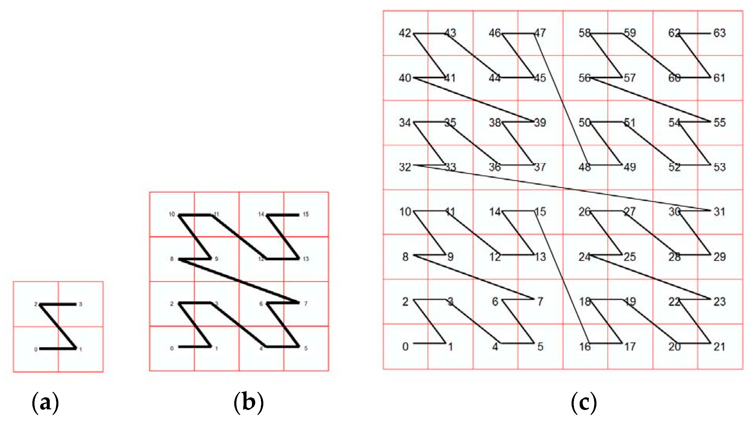
This paper enhances the area-based method developed in [12]. This method is based on the application of a space filling curve, which allow us to define a space tessellation (grid) as a mechanism for indexing the space (e.g., 2D or 3D). The subsequent linearization simplifies the treatment of 2D and 3D cases because they are converted to a 1D case. In addition, space filling curves are curves with other advantageous properties like self-similarity and hierarchy (see Figure 1 for the case of the Lebesgue curve).

It is important to highlight that, in [12], it was demonstrated that the method works well independently of the space-filling curve used. Continuing with the method, given a point pattern, point events are counted in each cell of the ordered tessellation and, after that, a multinomial law is considered to model the presence of the point events. In this way, we can compare two actual point patterns or a point pattern to a theoretical spatial distribution (e.g., a given point process). The comparison is developed based on a homogeneity test between the proportions (multinomial distributions) determined for each point pattern on the cells of the given grid.

The improvement introduced in this paper is motivated by the presence of empty cells in the grid. This fact may occur when the order of the curve increases or when we have a small or moderate number of events. Because small or zero observed proportions may affect the correct application of a test statistic for testing the null hypothesis desired, this problem is not a minor one, not only from the statistical point of view, but also from its applicability because obviating this problem can lead users to obtaining wrong conclusions. To overcome such a drawback, we consider for testing similarity of point patterns a test statistic belonging to the ϕ-divergence family. Two advantages of this choice are: first, the ϕ-divergences have been used for a wide variety of statistical problem because their good properties, especially in multinomial distributions. Examples in goodness-of-fit tests, homogeneity tests and model selection can be found in [13,14,15]. Secondly, the family of ϕ-divergences provides a great variety of test statistics depending on the function ϕ. Thus, appropriate ϕ will give us a way to deal with empty cells. In particular, we explore the usefulness of a test statistic based on the square Hellinger distance.

For this purpose, some simulation experiments are carried out and an illustration of the application to a real data set is included. First, the method is tested on several synthetic cases designed in order to analyze how the proposal works when we compare two similar HCFs (type I error), and what is the sensitivity of the proposal to distinguish between dissimilar HCFs (type II error). A base case is taken as a reference of HCF under the null hypothesis (H₀) and several parameters defining the base case are changed in order to carry out a study of the power of the method.

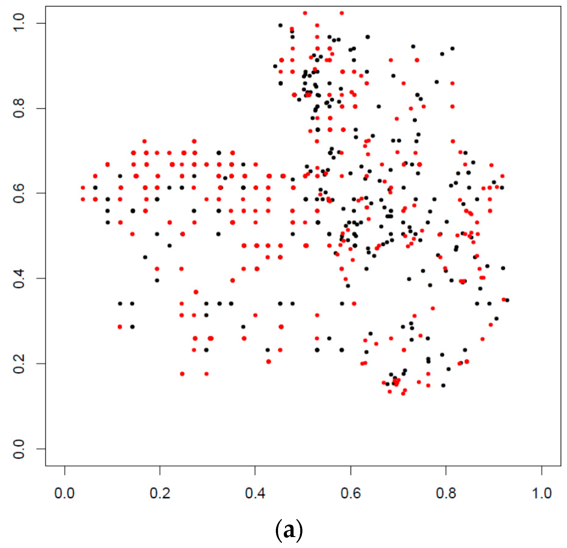
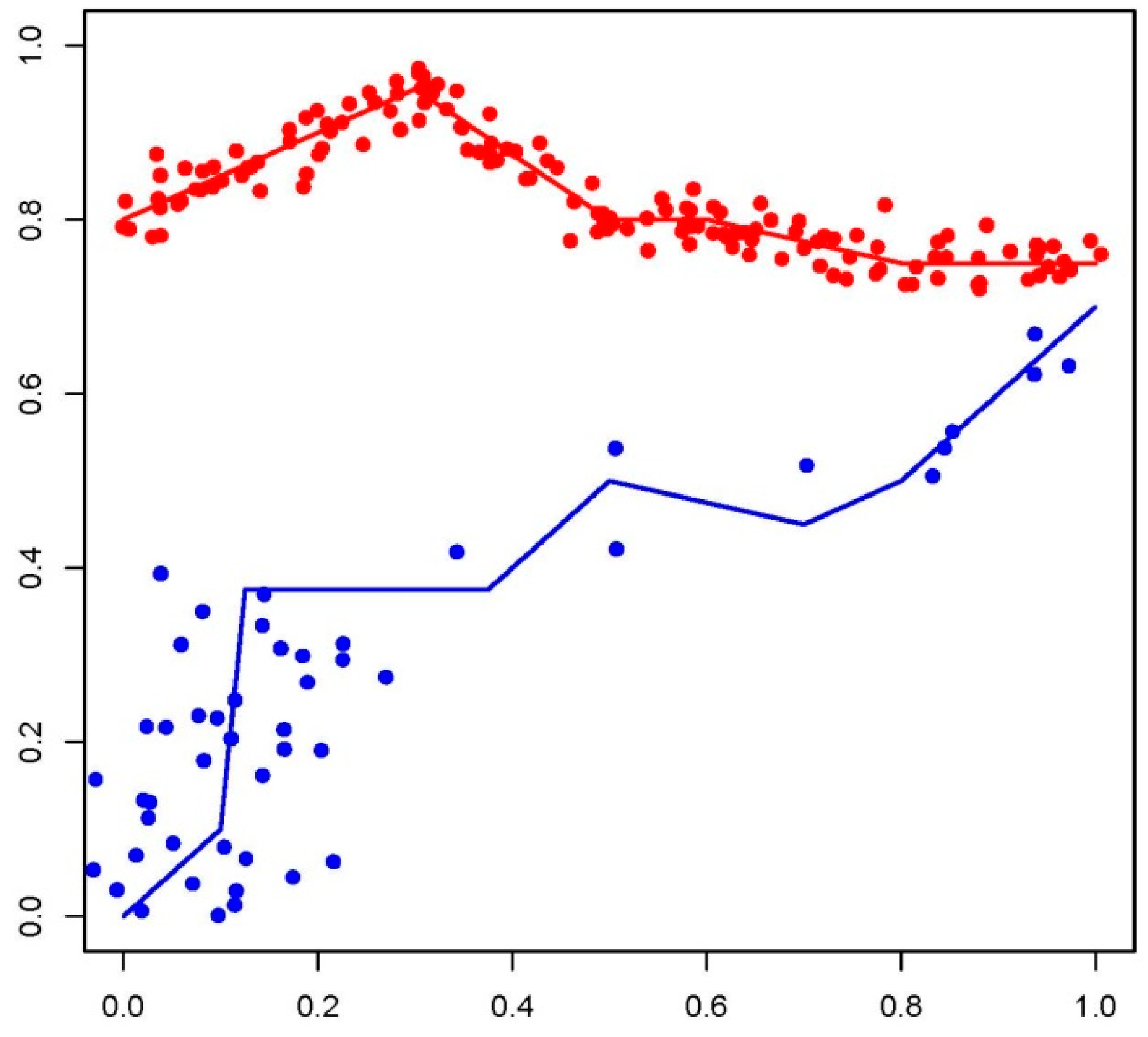
Second, in relation to its application to real data, we have used a dataset from [16] that comprises the distribution of fires by different causes and years in the region of “Castilla La Mancha” (Spain). According to this dataset, 3095 HCFs happened during 2004–2007, 1077 of them in 2004, 917 in 2005, 493 in 2006 and 608 in 2007, respectively. Because in Spain, late spring–summer is a seasonal period with a greater number of HCFs, we explore the effect of this fact in the spatial distribution of fires by means of the methodology proposed. For this task, we considered that each year is divided into two periods, say period 1 from May to September, and period 2 with the rest of the year. Figure 2 shows the distribution of HCFs for years 2004–2007. In this figure, the locations of fires corresponding to the period 1 appear in black and those corresponding to period 2 appear in red. Our proposal is oriented to answer questions like: Are these spatial distributions similar? The spatial distributions of fires are similar in late spring–summer and in the rest of the year? To answer this question, we do not need any statistical assumption about the underlying processes.

The rest of the paper is organized as follows. Section 2 introduces the method and main theoretical results of the homogeneity test for the multinomial distributions. Section 3 is devoted to present the synthetic case, Section 4 shows the results of the simulation experiments carried out to analyze the behavior of the proposal to overcome the problem of empty cells. Section 5 presents an application to a real dataset. Finally, Section 6 presents conclusions.

2. Methodology

Although the steps of the methodology were introduced in [12], here, we summarize the main ideas for the bivariate case. Let $X_{11},X_{12},\dots ,X_{1n}$ and $X_{21},X_{22},\dots ,X_{2m}$ be two independent samples of points from two spatial patterns with sizes n and m, respectively. Without loss of generality, let us suppose that both samples take values in the unit-square.

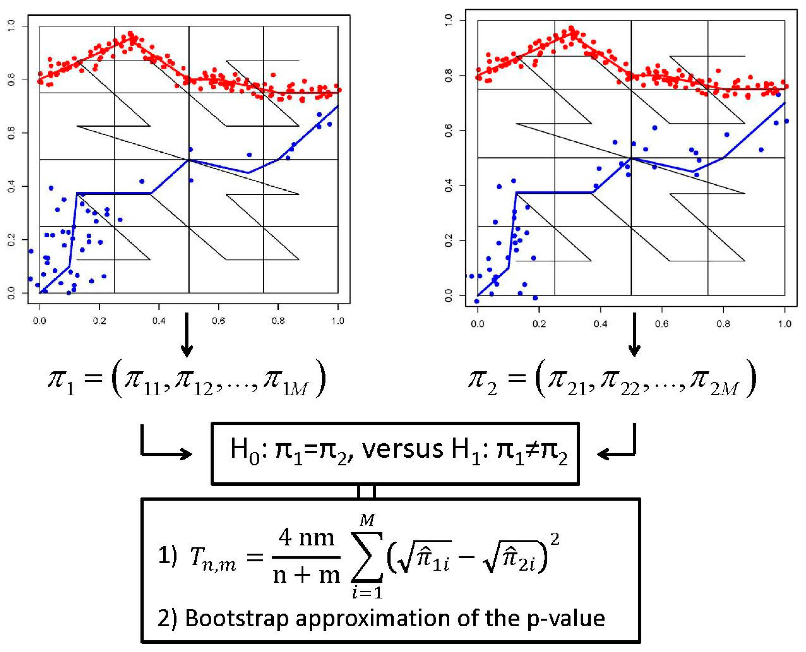
The methodology starts with the application of Morton’s curve to scan S for a particular order, ν, which induces a partition on S with M = 2^ν × 2^ν squares. The second part consists of assuming the distribution of points falling into the M cells of the grid can be modeled by a multinomial law. This way, after superimposing the tessellation to two point patterns, we obtain a realization of a multinomial distribution, and the problem of deciding whether both samples of points are similar is equivalent to the problem of testing whether the two multinomial distributions are the same. Next, we develop this idea.

Let ${\pi }_1={\left({\pi }_{11},{\pi }_{12},\dots ,{\pi }_{1M}\right)}^{\prime }$ and ${\pi }_2={\left({\pi }_{21},{\pi }_{22},\dots ,{\pi }_{2M}\right)}^{\prime }$ be the probability vector associated with each multinomial distribution where prime denotes transpose. The application of the curve to both samples of points provides us the proportions of points falling into each cell. Such proportions are the maximum likelihood estimators of multinomial parameters ${\pi }_{1i},{\pi }_{2i}, i=1,\dots ,M$, say ${\widehat{\pi }}_{1i}=\frac{n_{1i}}{n}, {\widehat{\pi }}_{2i}=\frac{n_{2i}}{m}$, i = 1, …, M. As a result, two HCFs will be considered as similar if the two underlying multinomial populations are equal. This fact is expressed as

H₀: π₁ = π₂, versus H₁: π₁ ≠ π₂.

(1)

Figure 3 gives a graphical summary of the methodology.

Although several choices are possible as a test statistic for testing ${\mathrm{H}}_0$, we have considered one based on ϕ-divergence. As said in the Introduction, from the initial works of Pearson or Matusita, extensive literature can be found about the use of statistics based on ϕ-divergence for inference purposes, and, in particular, for inference problems involving multinomial distributions. Here, we can make use of the fact that the square Hellinger distance is a particular case of a ϕ-divergence and hence shares the good statistical properties of this family, and, at the same time, it does not have a definition problem in the presence of zero values observed.

In particular, the square Hellinger distance between π₁ and π₂ is defined as

$$D\left({\pi }_1,{\pi }_2\right)={\displaystyle \sum }_{i=1}^M{\left(\sqrt{{\pi }_{1i}}-\sqrt{{\pi }_{2i}}\right)}^2.$$

(2)

$D\left({\pi }_1,{\pi }_2\right)\ge 0$ and it is equal to 0, if and only if, ${\pi }_1={\pi }_2$. Thus, by using the sample version of this distance, we consider the following test function for testing (1)

$$\mathsf{\Psi }=\{\begin{array}{cc}1,& \mathrm{if}{T}_{n,m}\ge t_{n,m,\alpha }\\ 0,& \mathrm{otherwise}\end{array}$$

(3)

where $T_{n,m}=\frac{4\mathrm{nm}}{n+m}{\sum }_{i=1}^M{\left(\sqrt{{\widehat{\pi }}_{1i}}-\sqrt{{\widehat{\pi }}_{2i}}\right)}^2$ and $t_{n,m,\alpha }$ is the 1 − α percentile of the null distribution of $T_{n,m}$.

A reasonable test for testing H₀ should reject the null hypothesis for “large” values of $T_{n,m}$. To be precise about what “large” values mean, we need to know the null distribution of $T_{n,m}$. In other words, we need to calculate the corresponding p-value, $p=P\left[T_{n,m}\ge T_{obs}\right]$, $T_{obs}$ being the observed value of the test statistic $T_{n,m}$ from the initial samples. Because the null distribution of $T_{n,m}$ is clearly unknown, one has to approximate it. One option is to consider its asymptotic null distribution, which is a chi-square variate with M-1 degrees of freedom (see [17] for theoretical details).

However, Refs. [18,19] have shown the chi-square approximation is rather poor for small and moderate sample sizes and the approximation of the null distribution by means of a parametric bootstrap estimator behaves better than the asymptotic one. Following these results, the p-value for testing (1) will be approximated by bootstrapping.

Hence, to evaluate the performance of this methodology, we can proceed as follows:

(1)

Given two point patterns, choose the value ν to construct Morton’s curve which will determine the tessellation of the space S and the number of cells M.

(2)

Count the number of points falling into each cell of the grid and obtain the observed relative frequencies ${\widehat{\pi }}_{1i}=\frac{n_{1i}}{n}, {\widehat{\pi }}_{2i}=\frac{n_{2i}}{m}$, i = 1, …, M.

(3)

Calculate $T_{obs}$ the observed value of $T_{n,m}$ from the initial samples of events.

(4)

Calculate the bootstrap p-value by means of Algorithm 1.

Algorithm 1. Bootstrap Algorithm

Step 1: Obtain $T_{obs}$ Step 2: Repeat for b = 1, …, B, (1) Generate two independent bootstrap sample of sizes n and m from the multinomial distribution under the null hypothesis, say, $M\left(n+m,{\pi }_0\right)$, where π0 is obtained from the pooled sample $${\widehat{\pi }}_{0i}=\frac{n{\widehat{\pi }}_{1i}+m{\widehat{\pi }}_{2i}}{n+m}, i=1,\dots ,M$$ (4) (2) Calculate the value of $T_{n,m}$ for each couple of bootstrap samples, say $T_{n,m}^{*b}$. Step 3: Approximate the p-value as $$p=\frac{Card\left(b: T_{n,m}^{*b}\ge T_{obs}\right)}{B}$$ (5)

3. Design of Synthetic Cases

The method is tested on synthetic cases designed in order to study two things: first, if we have two realizations of the synthetic case, the procedure is able to detect whether they are similar, or, equivalently, they come from the same multinomial distribution. This fact is known as the study of the type I error associated with the test function (3). Second, if we introduce some modifications in one of the two realizations, we are interested in evaluating if the procedure is able to distinguish them and hence detect whether they are similar point patterns because they represent different multinomial distributions. This issue is to evaluate the power of (3).

A synthetic base case is defined as a spatial structure of objects. With this structure of objects, we want to show that the method is capable of dealing with complex point patterns. Here, the synthetic base case is presented (Figure 4). Taking two structural elements of geography such as a road and a river, we have built a spatial distribution of points. This is only a simplistic example where two features act as the base of elementary point processes, but the situation can be made more complex by introducing more elements (e.g., settlements, railways, etc.) related to the fires caused by men. Why a road and a river? Some references indicate that fires occur near roads. In a nationwide study [20], it was determined that 95% of HCF occurred within 800 m of a road, and that over 90% of all wildfires from all causes occurred within 800 m of a road, also that less than 3% of all wildfires start in wilderness or backcountry areas more than 2 km from a road. Many recreational places are located near watercourses and it is demonstrated that recreational activities (e.g., vacationing, fishing, picnicking, hiking, setting barbecues, etc.) are fire causes [21,22]. Using the square unit as region of analysis (Figure 4), let consider a road (red line string) and a river (blue line string). The road is the base of a certain uniform point process that occurs in a buffer of the road with a certain width. The margins of the river are the paths for the excursions of the visitors of a recreational area that is downstream (lower left corner of the square unit). In this case, the length of the river has been divided in three sections and different widths and probabilities of HCF (due to different characteristics and facilities, e.g., picnic and barbecue facilities) can be assigned to each one. The lengths of the sections are L_RS1 = 0.25, L_RS2 = 0.30 and L_RS3 = 0.40 respectively. Given the spatial structure mentioned above, the parameters that define the base case (H₀) are the following:

• Number of HCF events. N_HCF = N_river + N_road, with the condition that N_road = 3 × N_river. This assignment is justified in that the road has a greater transit of vehicles than the river of visitors.
• Proportion of HCFs in each river section, P_RS1 = 0.80, P_RS2 = 0.05, P_RS3 = 0.15. This distribution of proportions is invented but is based on the following ideas: (1) visitors do not stray far from the recreational area and therefore the proportion of Section 1 is the largest; (2) Section 2 has very low probability as we consider that this is a stony and uncomfortable area for visitors; and (3) there are few visitors who arrive at the distant third section of the river.
• Buffer widths. The buffer widths, for the road and the river, are related to deviations. We have considered the condition D_river = 2 × D_road, and D_road = 0.03 (units in the square unit). This is an arbitrary decision for this example.

For the analysis of the type I error, we considered several N_HCF = (100, 200, 300, 400) and several orders of the space filling curve ν = (1, 2, 3) being applied to the base case (H₀).

For the power analysis (type II error), a set of alternative cases is used. Because there are several parameters defining the base model, in each alternative case, only one parameter is changed at a time, ceteris paribus. The alternative cases are:

Alternative cases #1. The road parameters of H₀ are fixed. The proportions in river sections are changed. The three options considered for the Alternative Case Proportions (ACP) are the following: ACP_op1 = (0.8 − a, 0.05 + a, 0.15); ACP_op2 = (0.8 − a, 0.05, 0.15 + a) and ACP_op3 = (0.8 − a, 0.05 + a/2, 0.1 + a/2), where a = (0.1, 0.2, 0.3). The deviation parameters of the river remain unchanged.

Alternative cases #2. The road parameters of H₀ are fixed. The proportions in river sections are fixed. Different values are considered for D_river = 0.06 ± a, where a = (0.01, 0.02, 0.03).

Alternative cases #3. The river parameters of H₀ are fixed. Different values are considered for D_road = 0.03 ± a, where a = (0.01, 0.02).

4. Performance of the Methodology

In this section, we will present the results of a simulation study carried out to evaluate the performance of the proposed methodology. As mentioned in the Introduction, in practical situations, it is common to find empty cells, especially for small and moderate sample sizes or when the number of cells in the grid increases. Thus, it is necessary to analyze how the methodology works when empty cells are present and the synthetic case described in Section 3 accommodates this idea.

Taking into account the previous premises, we first focus our attention on studying the type I error associated with the homogeneity test stated. In other words, we want to evaluate if the methodology works properly when both point patterns are similar. In our case, if we generate two realizations of the synthetic case, the methodology should identify if they are similar in the sense of representing the same underlying multinomial distribution.

Thus, we generated two point patterns of size n = m = 100 (N_road = 75 and N_river = 25) from the base case. We applied the proposal for ν = 1 and used the bootstrap algorithm to approximate the p-value with B = 1000 replications. We repeated this 5000 times and calculated the fraction of p-values less than or equal to the significance level α = 0.05, which represents the estimated type I error. The whole simulation was repeated for several sample sizes n = m = 200, 300, 400, and ν = 2, 3.

Table 1. Estimated type I error probabilities. HCF: Human caused fire.

Sample Sizes NHCF = Nroad + Nriver	ν = 1	ν = 2	ν = 3
100 (75 + 25)	0.057	0.060	0.075
200 (150 + 50)	0.048	0.055	0.057
300 (225 + 75)	0.049	0.052	0.055
400 (300 + 100)	0.050	0.054	0.056

shows the results obtained.

Looking at Table 1, it can be concluded that the estimated type I errors are close to the nominal value α = 0.05 in all cases tried. This fact means that the methodology concludes that two HCFs are similar when they really come from the same spatial pattern.

To complete the simulation study, we are interested in analyzing if the procedure is able to distinguish between point patterns properly. To do this, we have considered three types of alternatives explained in Section 3. The alternative cases #1 and #2 maintain the road parameters of H₀ fixed and pay attention to changes in the proportions in the river sections and in the deviations in the river, respectively, whereas the alternative case #3 pays attention to changes in the deviation of the road. All the alternative cases are indexed by the value of a, and, for each a, we generated a realization of the base case H₀ and a realization of the alternative case.

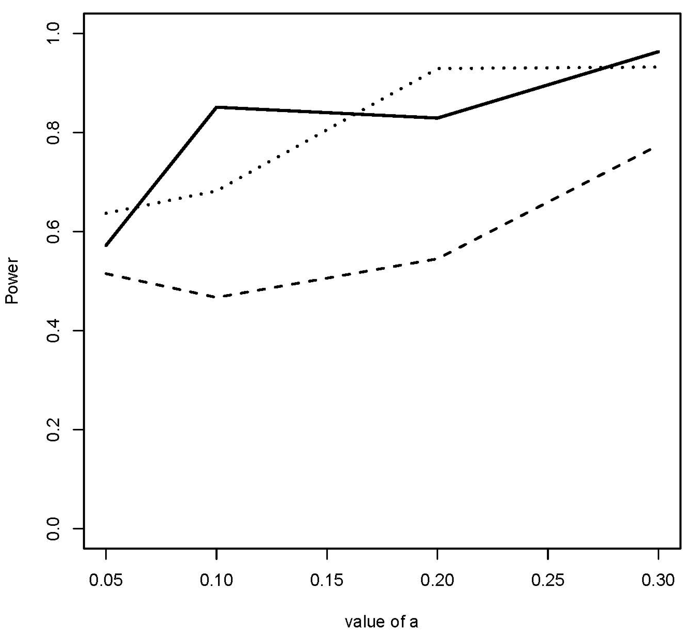
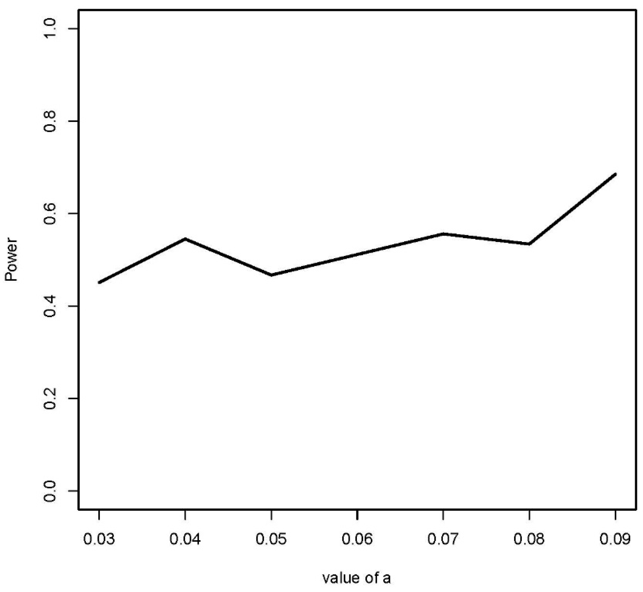
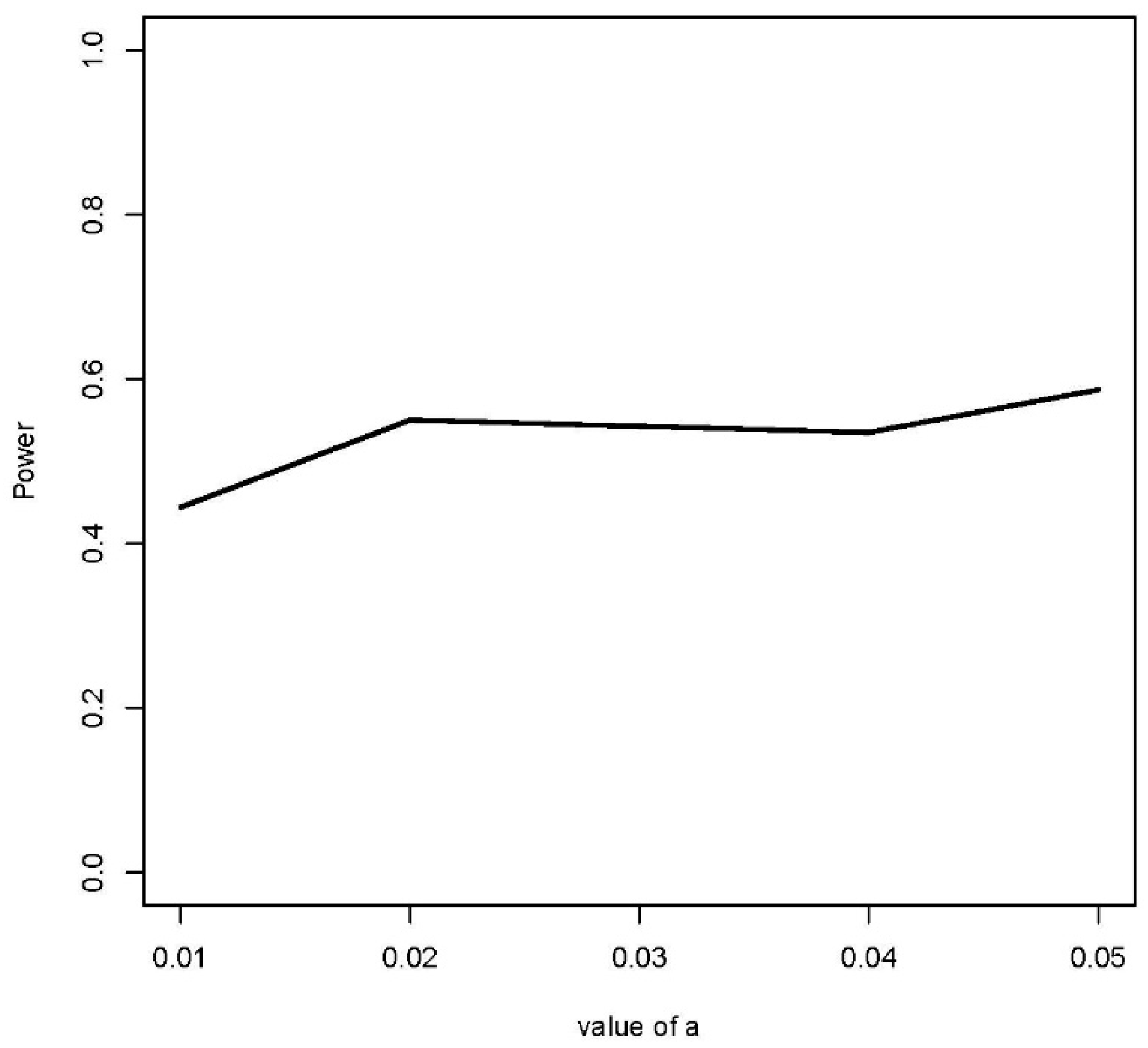
In this simulation experiment, we have fixed the order of Morton’s curve to ν = 2 and the sample sizes of the point patterns to n = m = 200 (N_road = 150 and N_river = 50). We repeated this 5000 times and calculated the fraction of p-values less than or equal to 0.05, which represents the power estimated for each alternative case at the signification level α = 0.05.

Figure 5, Figure 6 and Figure 7 show the estimated power for each type of alternative. Looking at these figures, the estimated powers are large in all the cases tried. In relation to case #1, the proposed method can distinguish them as different point patterns with small differences in proportions, on the order of 5%. In relation to cases #2 and #3, the same is valid for differences in buffer widths on the order of 1% of the square unit. Hence, it can be said the methodology works properly because it is able to distinguish between point patterns that represent different spatial point patterns.

5. Application to a Real Data Set

In this section, we illustrate the applicability of the proposal to study the similarity between two patterns of HCF. Coming back to the example mentioned in the Introduction, we have considered the dataset clmfires included in the spatstat package [16]. This data set comprises 3836 fire locations in the Spanish region called “Castilla La Mancha”, which happened from 2004 to 2007 (this region is approximately 400 by 400 km). According to the author of the package, these locations were recorded as exact UTM coordinates of the centroids of the fires. Some additional information is also provided: cause of fire, total area burned, date of fire. In addition, covariates (elevation, orientation, slope and land-use) are available as four pixel images. More information on the general method of data capture for the creation of the general statistics of fires in Spain can be seen in [23].

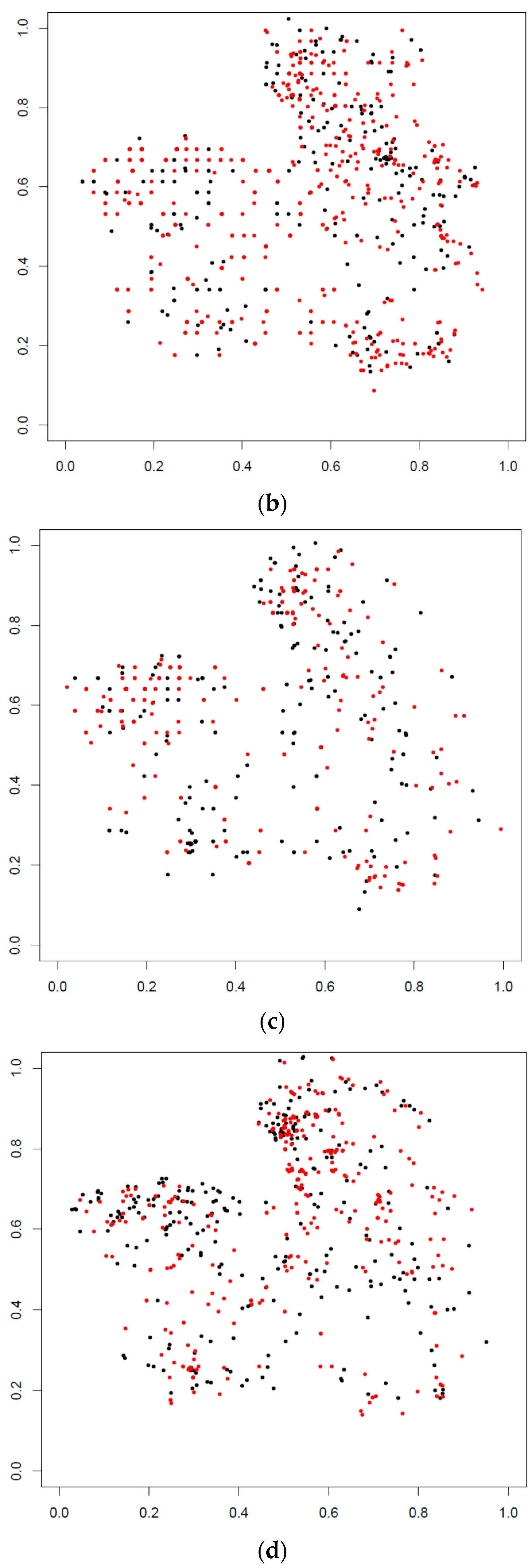
On the other hand, in Spain, there are two seasonal periods for which HCF patterns may vary spatially and temporally [24]. Thus, we paid attention to the spatial distribution of HCFs by year and by the two seasonal periods, say, from May to September (period 1) and the rest of the year (period 2) that are in black and red, respectively (see Figure 2), and by a combination of both.

Only 3095 of 3836 fire locations are HCFs.

Table 2. Number of HCF locations by years and by seasonal periods.

Year	Period 1	Period 2	Total of Fires
2004	698	379	1077
2005	443	474	917
2006	297	196	493
2007	314	294	608

summarizes the total of events by year and by period.

These sample sizes are large enough to apply the methodology by years, but taking into account the moderate sample sizes of some seasonal periods, we will consider ν = 2.

Table 3. Application of the proposal to HCFs in “Castilla La Mancha” (Spain). ** indicates statistical significance at 5% level.

Comparison	p-Value	Comparison	p-Value	Comparison	p-Value	Comparison	p-Value
Y2004–Y2005	0 **	P12004–P22004	0.178	P12004–P12005	0.001 **	P22004–P22005	0.005 **
Y2004–Y2006	0 **	P12005–P22005	0.003 **	P12004–P12006	0.002 **	P22004–P22006	0.036 **
Y2004–Y2007	0 **	P12006–P22006	0.295	P12004–P12007	0 **	P22004–P22007	0 **
Y2005–Y2006	0.001**	P12007–P22007	0 **	P12005–P12006	0.074	P22005–P22006	0.131
Y2005–Y2007	0.004 **			P12005–P12007	0.008 **	P22005–P22007	0.071
Y2006–Y2007	0.003 **			P12006–P12007	0.522	P22006–P22007	0 **

shows the approximated p-values for the comparisons carried out with B = 1000 bootstrap replications. For a better understanding of such comparisons, the notation used is Y₂₀₀₄ to identify the total HCFs of year 2004, P1₂₀₀₄ represents the sample of HCFs corresponding to period 1 for the year 2004 and P2₂₀₀₄ denotes the HCFs that happened in period 2 for the year 2004, so on and so forth.

Recall the null hypothesis to be tested is the similarity of HCFs. Thus, to make the interpretation of p-values easier, ** indicates statistical significance at 5% level.

The application of the proposal concludes that the comparisons by years exhibit dissimilarity between point patterns of fire locations. Focusing on the comparison between seasonal periods, the fire locations of both periods are similar only for the years 2004 and 2006. Finally, by combining the comparisons by year and by period, the years 2005 and 2006 (same for years 2006 and 2007) have similar point patterns of fires in period 1. However, for period 2, we can say the HCFs between 2005 and 2006 and between 2005 and 2007 are similar. The rest of the comparisons carried out conclude dissimilarity between fire locations.

From the perspective of HCF management, the fact that a set of years or periods can be considered similar signifies the presence of a similar spatial pattern in terms of the risk of fire (possibility of fire starting due to the presence of causative agents [25]). This may indicate the existence of some pattern in the cause of HCFs with results in the presence of fire-prone areas. In addition, if there is a common pattern, the logical thing is to guide the management activities to eliminate, or at least reduce as much as possible, the assignable causes of the HCFs. The proposed statistical method does not relate causes or covariates with HCFs, or between HCFs. It only analyzes the presence of HCFs in the space, and the space means many structural variables (e.g., vegetation, land use, slope, aspect, proximity, etc.). This means that you must know the territory (structural variables), and what happened in it very well, in order to be able to draw conclusions. However, the presence of a common pattern would allow zoning and actions focused on zones. Ref. [25] points out that the risk of fire is one factor that managers should consider in managing forests in order to propose fire protection programs. Specific fire prevention (e.g., fuel treatment practices, firebreaks, distribution of firefighting resources, etc.) [26], detection, suppression (e.g., evacuation and coordination strategies) [27], and post-fire effects’ strategies (e.g., post-fire vegetation recovery), will depend on each specific case under analysis.

Conclusions are reached in a statistically simple way and do not require a previous distributional hypothesis. Of course, it is not an explanatory method of why the spatial point patterns are as they are, or why they are similar or different. This method simply indicates that statistically they can be considered as equal or different, which for some aspects of fire management is sufficient as a starting point for further investigations.

6. Conclusions

Results indicate that a new robust and sensitive method for comparing spatial point patterns of human caused fires is available. In short, some strengths of this method are:

(1)

It is robust because no underlying hypothesis is needed for the comparison of the spatial point pattern of the HCF events.

(2)

The spatial indexing system simplifies the work with two-dimensional spaces (in general, nD) using a conventional one-dimensional statistical tool.

(3)

The statistical base is the multinomial law, a very well-known statistical distribution function, easy to understand and to apply.

(4)

Over-dispersed spatial data is frequent in practice and the presence of empty cells occurs as it is shown in the synthetic case. This fact provokes that some statistical tools may be used improperly and hence provides misleading conclusions. Thus, it is necessary to have a statistical procedure able to overcome this problem as we have made for the homogeneity test of multinomial distributions.

(5)

The use of the square Hellinger distance as the base of the test statistic for comparing the two observed event distributions has demonstrated the capability for dealing with over-dispersed spatial data.

(6)

The use of synthetic cases has shown that the method is able to conclude that two point patterns of fires are similar when they really are, and it is sensitive to the possible changes between two spatial distributions (quantity, dispersion, spatial distribution, etc.). In addition, the synthetic cases have provided evidence that the method works well with relatively small samples of events.

From an applied point of view, the presence of ignitions has been used as example, so that a similar spatial distribution (similar spatial pattern) can be considered as the existence of the same risk of fire and the same causes. The verification of this circumstance allows zoning and focuses on the possible actions of the management of HCFs. In addition, note the two samples of ignitions to be compared can be defined by focusing on an aspect of interest—for instance, the presence of roads, rivers or proximity to recreational areas (as shown by the synthetic cases), and, in a more general way, the period of time (year, month, seasonal period), the cause of fires (lightning, accident, intentional cause), among many other situations. Anyway, by comparing two desired scenarios, the conclusion of the statistical tool will indicate if this selected aspect is relevant to explain the observed locations of events in the following sense: if the two multinomial distributions are the same, this aspect does not have an influence on the spatial location of HCFs (similar point patterns). On the contrary, if the two multinomial distributions are different, this aspect should explain the differences in the spatial location of ignitions (for instance, presence of roads, proximity to recreational areas, period of time, and so on).

Thus, at the management level, this statistical tool can be useful to identify explanatory variables about how spatial distributions of fire locations are and how they vary.