Article

Additive Biomass Equations Based on Different Dendrometric Variables for Two Dominant Species (Larix gmelini Rupr. and Betula platyphylla Suk.) in Natural Forests in the Eastern Daxing’an Mountains, Northeast China

1
Department of Forest Management, School of Forestry, Northeast Forestry University, Harbin 150040, China
2
Department of Forest and Natural Resources Management, State University of New York, College of Environmental Science and Forestry (SUNY-ESF), One Forestry Drive, Syracuse, NY 13210, USA
*
Author to whom correspondence should be addressed.
Forests 2018, 9(5), 261; https://doi.org/10.3390/f9050261
Submission received: 16 April 2018 / Revised: 1 May 2018 / Accepted: 6 May 2018 / Published: 10 May 2018
(This article belongs to the Section Forest Ecology and Management)

Abstract

:
A total of 138 Dahurian larch (Larix gmelinii Rupr.) trees and 108 white birch (Betula platyphylla Suk.) trees were harvested in the eastern Daxing’an Mountains, northeast China. We developed four additive systems of biomass equations as follows: the first additive model system (MS-1) used the best combination of tree variables as the predictors; the second additive model system (MS-2) included tree diameter at breast height (D) as the sole predictor; the third additive model system (MS-3) included both D and tree height (H) as the predictors; and the fourth additive model system (MS-4) included D, H, and crown attributes (crown width (CW) and crown length (CL)) as the predictors. The model coefficients were simultaneously estimated using seemingly unrelated regression (SUR). The heteroscedasticity in model residuals was addressed by applying a unique weight function to each equation. The results indicated that: (1) the stem biomass accounted for the largest proportion of the total tree biomass, while the foliage biomass had the smallest proportion for the two species; (2) the four additive systems of biomass equations exhibited good model fitting and prediction performance, of which the model Ra2 > 0.81, the mean prediction error (MPE) was close to 0, and the mean absolute error (MAE) was relatively small (<9 kg); (3) MS-1 and MS-4 significantly improved the model fitting and performance; the ranking of the four additive systems followed the order of MS-1 > MS-4 > MS-3 > MS-2. Overall, the four additive systems can be applied to estimate individual tree biomass of both species in the Chinese National Forest Inventory.

1. Introduction

Biomass is an important characteristic of forest ecological systems. The accurate quantification of tree biomass is critical and essential for studying carbon storage, climate change, forest health, forest productivity, fuel (and bioenergy), nutrient cycling, etc. [1,2,3,4,5]. Although direct measurement of the actual weight of each tree component (i.e., stem, branch, foliage, and root) is undoubtedly the most accurate method, it is destructive, time-consuming, and costly. Therefore, developing biomass models is considered a better approach for estimating forest biomass [6,7,8].
To date, hundreds of biomass equations have been developed for more than 100 species worldwide [9,10,11,12,13,14]. However, most studies have focused on aboveground biomass, while relatively few studies have attempted to study belowground (or root) biomass, because excavating tree roots is extremely difficult and expensive [15,16,17].
In forest ecosystems, the biomass of small trees (diameter at breast height <5 cm) constitutes an essential component of the total forest biomass. Unfortunately, in most empirical studies, the forest biomass calculations have ignored small trees, consequently underestimating the totality of the overall values [18,19]. Researchers have recently reported that small-diameter trees can play a substantial role in the estimation of total biomass and bioenergy, because these small-diameter trees compose a significant proportion of the tree population and can grow more rapidly than larger-diameter trees [2,20,21]. However, there is no study that investigated the development of biomass equations including small-diameter trees in the temperate forests of the eastern Daxing’an Mountains in northeast China.
In general, tree diameter at breast height is the commonly used and reliable sole predictor of total, subtotal, and component biomass in most biomass equations [5,15,22]. Furthermore, depending on research goals, other tree variables (e.g., tree height, crown length, and crown width) have been investigated as potential predictors for tree biomass modeling [23,24,25,26]. Despite these tree variables being much more difficult to obtain in practice, studies have shown that different tree height, crown length, and crown width for the same tree diameter at breast height clearly influence tree-level biomass equations. Including tree height, crown length, and/or crown width into biomass equations as the additional predictors can significantly improve model fitting and performance, explain more sources of variation in the data, and avoid potential limitations [5,8,24,26,27,28,29].
The biomass equations for estimating the total, subtotal, and component biomass of trees can be classified as non-additive or additive in nature. Non-additive biomass equations fit the total, subtotal, and component biomass data separately. Consequently, the sum of model predictions from the component biomass models may not be equal to the model prediction from the total biomass models. On the other hand, additive biomass equations fit the total, subtotal, and component biomass data simultaneously to account for the inherent correlations among biomass components measured on the same sample trees [6,22,24]. Thus, the sum of biomass predictions from the component biomass equations is equal to the biomass predictions from the total or subtotal biomass equations [30,31]. To ensure the additivity for a system of biomass equations, various model specification and parameter estimation methods have been proposed for both linear and nonlinear biomass equations [6,30,31,32]. In particular, seemingly unrelated regression (SUR) and nonlinear seemingly unrelated regression (NSUR) are more general and flexible, and they have become more popular as the parameter estimation methods for linear and non-linear biomass equations. Several recent applications of the SUR method have been reported to ensure the additivity in the nonlinear simultaneous equation systems of tree biomass [6,22,24,33,34].
Tree biomass data often show heteroscedasticity in model residuals. To overcome this problem, a weighted regression or logarithmic transformation should be defined and used for each biomass model. With respect to logarithmic regression, a fitted logarithmic model provides the prediction of log(Y). However, the anti-log transformation from log(Y) to Y introduces bias, and the correction on the bias is necessary. To obtain the desired prediction of Y, the predicted values of Y should be adjusted in some manner, such as being multiplied by a correction factor. Several correction factors have been proposed and applied over the last decades [35,36,37]. When the model error term is sufficiently small, the correction factor may not be necessary, but the correction factor cannot be ignored when the model error term is relatively large [38,39]. In general, logarithmic regression is simple and may be better for developing biomass equations when the sample sizes are small. Unfortunately, after a correction factor is applied to the additive system of logarithmic equations, the property of additivity may be damaged among the total, subtotal, and component biomass equations [22]. When the sample sizes are relatively large, weighted regression can be used to directly overcome the heteroscedasticity in the residuals of total and component biomass models [7,24].
Since the cold temperate forests in the eastern Daxing’an Mountains in northeast China were excessively harvested from the 1960s to 2000s, many young and middle-aged forests now exist in the region. The current cold temperate forests play an important role not only in the national carbon storage and budget, but also in the recovery of biodiversity following harvest or wildfires. Dahurian larch (Larix gmelinii Rupr.) and white birch (Betula platyphylla Suk.) are the two dominant species in the natural forests of the eastern Daxing’an Mountains. However, the Chinese National Forest Inventory lacked accurate systems of tree biomass models for Dahurian larch and white birch, and only a few studies have investigated the aboveground and belowground biomass of these species in China. Wang [15] and Mu et al. [40] developed biomass equations for both species in northeast China, but their biomass data were collected from a limited forest region and originated from a relatively small sample size (e.g., two dominant, three codominant, three intermediate, and two suppressed trees) for both species. Moreover, the established biomass equations were non-additive. Dong et al. [8,22] constructed two additive systems of biomass models for several conifer and hardwood species (including Dahurian larch and white birch) in the Xiaoxing’an Mountains, but did not include trees <5.4 cm. Meng et al. [28] used data from 48 trees to construct additive biomass models for white birch in the western Daxing’an Mountains (eastern Inner Mongolia), but the developed models were not applicable to belowground (root) biomass. In addition, few studies have focused on biomass equations for Dahurian larch and white birch in the eastern Daxing’an Mountains. Overall, accurate systems of biomass equations for cold temperate forests across the eastern Daxing’an Mountains in northeast China have not been developed.
The objectives of this study were as follows: (1) compare biomass models based on different predictors of total, aboveground, root, stem, crown, branch, and foliage biomass for Dahurian larch and white birch trees in the eastern Daxing’an Mountains; (2) use SUR to construct four additive systems (i.e., one-, two-, three- and best-variable systems) of biomass equations with three constraints and overcome the heteroscedasticity problem; (3) use the jackknife technique to validate the performance of the biomass models; (4) evaluate the different methods of quantifying tree-level biomass; and (5) compare the newly developed additive biomass equation system against the biomass equations published in the literature.

2. Materials and Methods

2.1. Study Sites

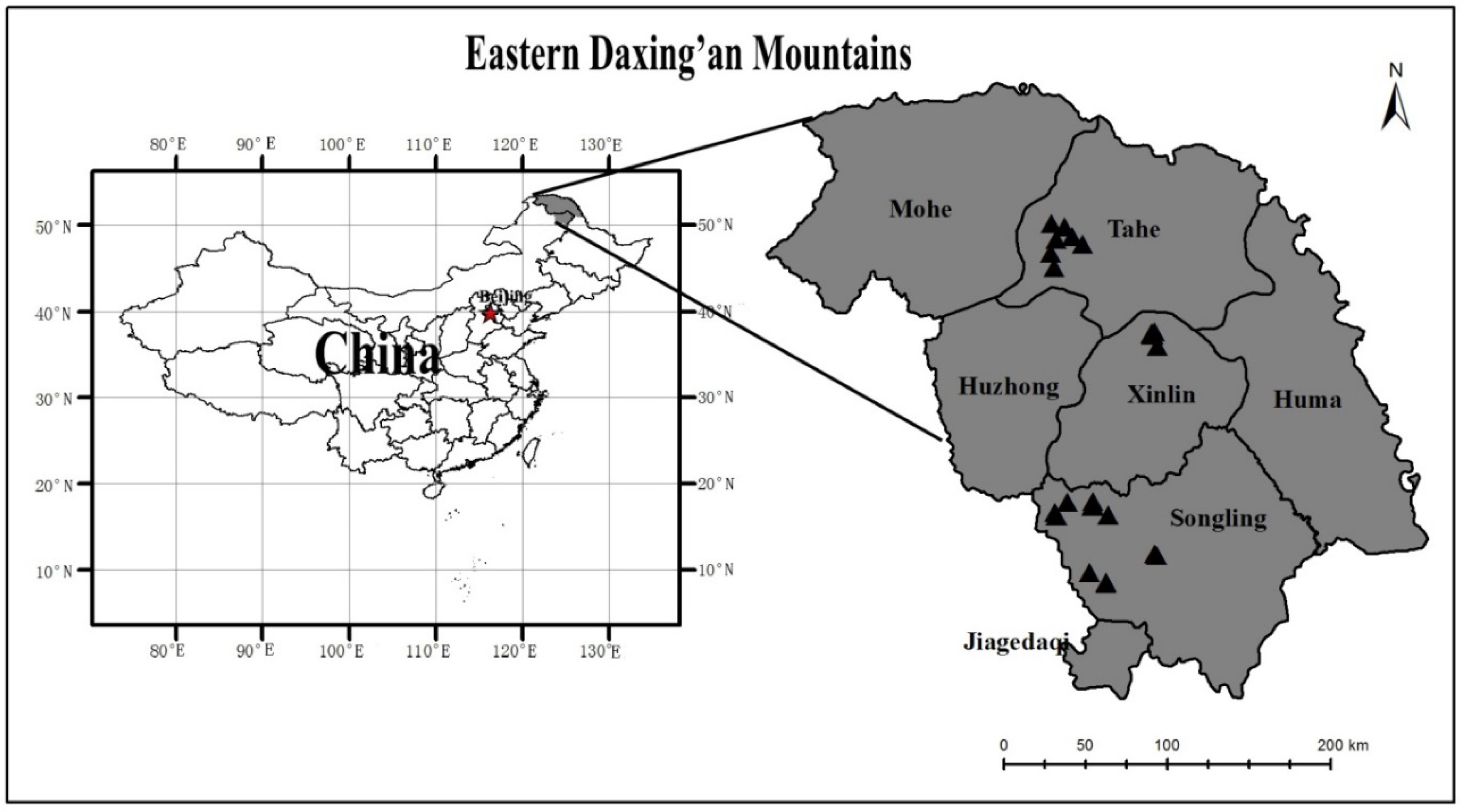
This study was conducted in the eastern Daxing’an Mountains in northeast China (from 121°12′ E to 127°00′ E and from 50°10′ N to 53°33′ N). The total area of the region is 83,000 km2, and the altitude ranges from 300 to 1520 m above the sea level (Figure 1). The soils are mostly Umbri-Gelic Cambosols according to the Chinese taxonomic system [41]. This area is associated with a distinct cold temperate continental monsoon climate: the mean annual air temperature ranges from −1 to −2.8 °C; the mean air temperatures in January and July are −28 °C and +20 °C, respectively; and the mean annual rainfall ranges from 500 to 750 mm. Dahurian larch (Larix gmelinii) and white birch (Betula platyphylla) are the dominant tree species, accompanied by aspen (Populus davidiana Dode.) and Mongolian pine (Pinus sylvestris var. mongolica). The understory and ground vegetation are dominated with blueberry (Vaccinium angustifolium Aiton), Rhododendron dahuricum L., and Ledum palustre L., among others.

2.2. Plot Measurements and Biomass Estimation

The data used in this study were selected from a large data set of tree biomass. The tree species included Dahurian larch and white birch in the young and middle-aged natural forests of the eastern Daxing’an Mountains in northeast China. The sample plots were established in August of 2012, 2013, 2014, 2015, and 2016. A total of 31 plots were selected, including 18 plots of Dahurian larch forest, 4 plots of white birch forest, and 9 plots of Dahurian larch and white birch mixed forest. Each plot was 20 × 50 m in size. The characteristics of the forest types are listed in Table 1. For each of the 31 plots, at least one sample tree for each of the dominant, intermediate, and suppressed trees were targeted. In addition, some small sample trees (diameter at breast height <5 cm) were selected outside of the 31 plots. In total, 138 Dahurian larch trees and 108 white birch trees were destructively sampled (Table 2).
The targeted sample trees were cut at the ground. Tree measurements, including tree diameter at breast height (D), tree height (H), crown width (CW), and crown length (CL), were measured and recorded. Among them, H and CL were measured after cutting, while D and CW were measured before cutting. The live crown, which constitutes the first dead branch to the base of the terminal bud, was divided equally into three layers: top, middle, and bottom. All live branches within each crown layer were cut and weighed. Then, 1–2 branches were selected from each crown layer, and the branches and foliage were separated and weighed. The samples (approximately 50–100 g) of the branches and foliage were collected, weighed, and taken to the laboratory to determine their moisture content. The stems of each sample were cut into 1-m sections, after which, each section was weighed and recorded. At the end of each stem section, a 2–3-cm thick disc was cut, weighed, and taken to the laboratory to determine its moisture content and analyze its growth rings to determine tree age with WinDENDRO software (Regent Instruments, Inc., Québec, QC, Canada). The roots of large trees were excavated using a combination of chains (i.e., lifting equipment) and manual digging. However, the roots of small trees were removed manually. Because most fine roots were out of the working zones (approximately 3 m in radius), and excavating the fine roots is difficult, costly, and time consuming, the fine roots (diameter < 5 mm) were excluded in this study. The roots of the sampled trees were divided into large roots (diameter ≥ 5 cm), medium roots (diameter 2–5 cm), and small roots (5 mm < diameter < 2 cm). The root diameters were measured with a digital caliper. The root samples in each class were sampled (approximately 100–200 g), weighed, and then taken to the laboratory to determine their moisture content. All stem, branch, foliage, and root samples were oven-dried at 80 °C and then weighed. The dry biomass of each component was calculated by multiplying the fresh weight of each component by the dry weight-to-fresh weight ratio of that component. For each sampled tree, the sum of large, medium, and small root dry biomass yielded the root dry biomass. The sum of the branch dry biomass and foliage dry biomass yielded the crown dry biomass. The sum of the crown dry biomass and stem dry biomass equaled the aboveground biomass, and the sum of the aboveground dry biomass and the root dry biomass equaled the total tree biomass.
A summary of the descriptive statistics for D, H, CL, and CW as well as the total, subtotal, and component biomass of trees is shown in 
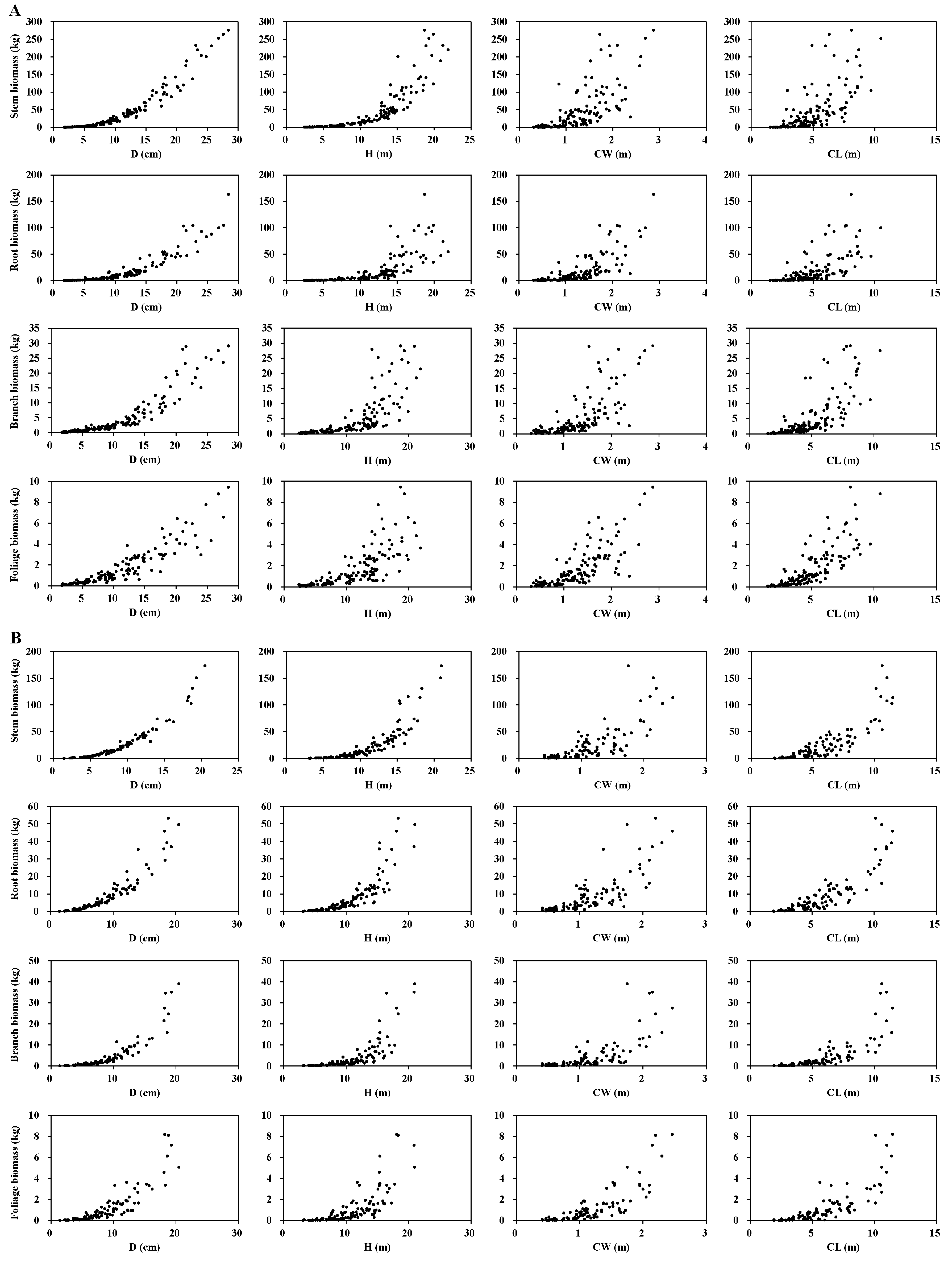
Table 2. The stem, branch, foliage, and root biomass of all sample trees as well as their relationships with D, H, CL, and CW are shown in Figure 2. We performed statistical tests (e.g., dummy variable regression) to confirm that there was no significant difference between young and middle-age trees for the total, stem, root, and foliage biomass of two species, with the exception of branch biomass. Therefore, the sampled trees from different diameter classes (or different ages) were combined for data analysis and model development in this study.

2.3. Systems of Additive Biomass Equations

2.3.1. Model Selection

Visual inspection of the stem, branch, foliage, and root biomass data indicated that the component biomass of trees can be modeled as a multivariable allometric model of tree variables (Figure 2). The general tree biomass equation in this study is nonlinear with an additive error term as follows:
W i = β i 0 X 1 β i 1 X 2 β i 2 X k β ik + ε i
where Wi represents the root, stem, branch, foliage, aboveground, crown, and total tree biomass in kilograms (i = r, s, b, f, a, c, and t for root, stem, branch, foliage, aboveground, crown, and total, respectively); Xj represents various tree variables (j = 1, …, k), such as D, H, CL, and CW, respectively; βij represents the model parameters to be estimated; and εi is a model additive error term. From the general Equation (1), we proposed the following biomass models based on the different combinations of predictors of tree component biomass:
W i = β i 0 D β i 1 + ε i
W i = β i 0 ( D 2 H ) β i 1 + ε i
W i = β i 0 D β i 1 H β i 2 + ε i
W i = β i 0 D β i 1 H β i 2 CW β i 3 + ε i
W i = β i 0 D β i 1 H β i 2 CL β i 3 + ε i
W i = β i 0 D β i 1 H β i 2 CW β i 3 CL β i 4 + ε i
The total, subtotal (i.e., aboveground and crown), and component biomass of tree equations may have different combinations of predictor variables. We fit each of the above nonlinear equations to the total biomass, subtotal biomass, and component biomass (i.e., stems, branches, foliage, and roots) of trees, respectively. A “best model” was selected for each of the total, subtotal, and component biomass based on the model fitting statistics such as adjusted coefficient of determination (Ra2), root mean squared error (RMSE), and Akaike information criterion (AIC). Finally, we decided to use the best-, one-, two-, and three-predictor biomass models as the basic model formats to construct four candidate additive systems of biomass equations that each has three constraints. In four candidate additive systems, the biomass models of tree components were constrained to equal the (1) total tree biomass, (2) aboveground biomass, and (3) crown biomass.

2.3.2. Additive Biomass Equations

Following the model structure specified by Parresol [31], the additive systems of seven equations with cross-equation constraints on the structural parameters and cross-equation error correlations for root, stem, branch, foliage, subtotal (i.e., crown and aboveground), and total biomass are specified as:
{ W r = β r 0 X 1 β r 1 X 2 β r 2 X k β rk + ε r W s = β s 0 X 1 β s 1 X 2 β s 2 X k β sk + ε s W b = β b 0 X 1 β b 1 X 2 β b 2 X k β bk + ε b W f = β f 0 X 1 β f 1 X 2 β f 2 X k β fk + ε f W c = W b + W f + ε c W a = W s + W b + W f + ε a W t = W r + W s + W b + W f + ε t
where Wr to Wt represent the vectors of the root, stem, branch, foliage, crown, aboveground, and total biomass in kilograms, respectively.
To overcome the heteroscedasticity in the residuals of the biomass models, a weight function should be defined and used for each biomass model, such as the total, subtotal, and tree component biomass equations. The error variance of the ith observation is functionally related to one or more of the predictor variables and can be modeled as a power function of the predictor variables, as in σ i 2 = σ 2 ( X 1 γ i 1 X 2 γ i 2 LX k γ ik ) [30,42], where the power coefficient γik can be obtained by stepwise regression using the logarithmic form of the error variance model e i 2 = σ 2 ( X 1 γ i 1 X 2 γ i 2 X k γ ik ) , in which e i is the model residual of the unweighted model. Hence, we chose 1 / X 1 γ i 1 X 2 γ i 2 X k γ ik as the weight function, and γik was determined for each biomass model. In the computations, the weight function for heteroscedasticity 1 / X 1 γ i 1 X 2 γ i 2 X k γ ik was multiplied and programmed using the PROC MODEL procedure in SAS by specifying resid. W i = resid . W i / X 1 γ i 1 X 2 γ i 2 X k γ ik [43].

2.3.3. Model Assessment and Validation

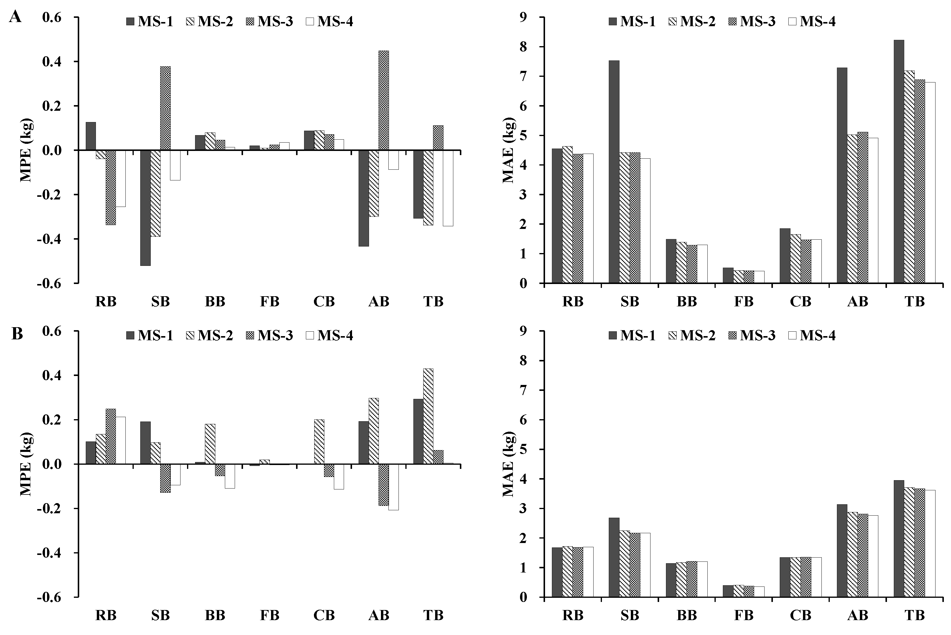
The four additive systems of biomass models were fitted to the entire data set, and the models were validated using the jackknife technique, in which a biomass model was constructed using all but one observation (sample size N − 1). Afterward, the fitted model was used to predict the value of the dependent variable for the excluded observation. Four statistics that were based on jackknifing and that were obtained for each system equation were used to evaluate the model fitting (Ra2 and RMSE) and performance (mean prediction error (MPE) and mean absolute error (MAE)) for each biomass prediction system, where MPE represents the average prediction error, and MAE represents the magnitude of prediction error.
The mathematical expression of the four statistics is displayed as follows:
Adjusted   coefficient   of   determination   R a 2 = 1 i = 1 N ( W i W ^ i ) 2 i = 1 N ( W i W ¯ ) 2 ( N 1 N p )
Root   mean   squared   error   RMSE = MSE = i = 1 N ( W i W ^ i ) 2 N p
Mean   prediction   error   ( MPE )   MPE = i = 1 N ( W i W ^ i , i ) N
Mean   absolute   error   ( MAE )   MAE = i = 1 N | W i W ^ i , i | N
where W i is the ith observed biomass value, W ^ i is the ith predicted biomass value from the model that was fitted using all data (sample size N), W ¯ is the mean of the biomass value, W ^ i , i is the predicted value of the ith observed value by the fitted model that was fitted by (N − 1) observations and that excluded the use of the ith observation, and p is the number of model parameters.
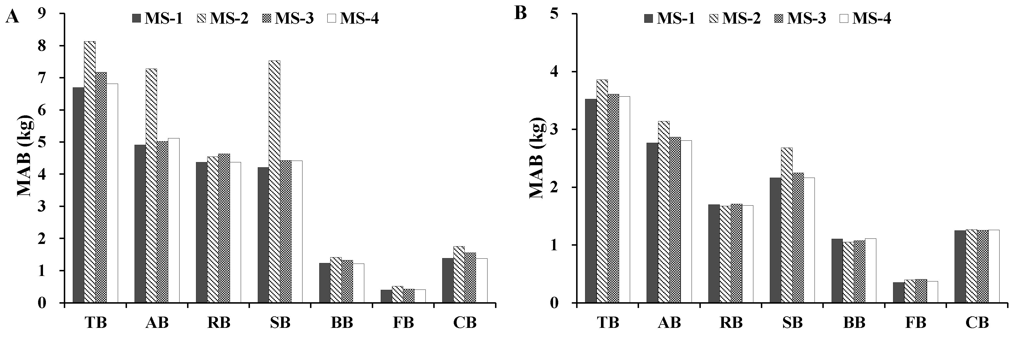
In addition, we calculated the mean absolute bias (MAB) to compare the newly developed additive biomass equation systems against the biomass models published in the literature.
Mean   absolute   bias   ( MAB )   MAB = i = 1 N | W i W ^ i | N

2.3.4. Model Estimation and Data Analysis

For the above four additive systems of biomass equations, PROC MODEL procedure in SAS [43] was used to simultaneously estimate the coefficients of the tree component biomass models. To analyze the partitioning of tree biomass into basic components, the fitted models were used to partition across 5-cm diameter classes. The analysis of variance (ANOVA) of the PROC GLM procedure in SAS software [43] was used to test the differences between the four additive systems to estimate the total and component biomass at the individual tree level as well as at the plot level followed by the contrasts between the four additive systems.

3. Results

3.1. Selection of Best Tree Biomass Equations

In this study, the tree variables D, H, CL, and CW were fitted to each of the total, subtotal (i.e., aboveground and crown), and tree component (i.e., roots, stems, branches, and foliage) biomass data. Table 3 shows the model fitting statistics, including Ra2, RMSE, and AIC. The incorporation of H into the biomass models significantly improved the model fitting for the total and tree component biomass models as a result of the smaller RMSE and AIC for both tree species (Table 3). For Dahurian larch, CW was highly significant in the root, stem, and foliage biomass equations, while CL was a significant predictor in the branch and foliage biomass equations. For white birch, CL was a significant predictor in the stem and foliage biomass equations, while CW was a significant predictor in the stem and foliage biomass equations. Overall, Equations (4) and (5) were selected as the best root biomass equations for Dahurian larch and white birch, respectively. Similarly, Equations (6) and (7) were the best stem biomass equations for Dahurian larch and white birch, respectively, Equations (4) and (6) were the best branch biomass equations for Dahurian larch and white birch, respectively; and Equation (7) was the best foliage biomass equation for both Dahurian larch and white birch.

3.2. Model Fitting for Additive Biomass Equations

Based on the best root, stem, branch, and foliage biomass equations, the SUR method was used to fit the additive systems of all tree component biomass, subtotal biomass, and total biomass (MS-1) to the biomass data for Dahurian larch (Equation (14)) and white birch (Equation (15)). The additivity was guaranteed by setting three constraints to the parameters of the additive systems of the biomass equations in this study. The coefficient estimates, standard errors (SEs) and goodness-of-fit statistics (i.e., Ra2 and RMSE) of the additive system of biomass equations based on the best predictors (MS-1) for both tree species obtained by SUR are shown in Table 4. The results indicated that all equations in MS-1 fit the biomass data well: Ra2 > 0.86 and RMSE < 12.00 kg. The best model fittings were obtained from the total, aboveground, and stem biomass equations, while the worst model fittings were obtained from the foliage and branch biomass equations, which presented relatively lower Ra2 values and larger RMSE values (Table 4). For each biomass equation of both tree species, the weight function involved D or a combination of D plus H, CW, or CL (Table 4).
{ W r = e β 10 D β 11 H β 12 CW β 13 + ε r W s = e β 20 D β 21 H β 22 CW β 23 CL β 24 + ε s W b = e β 30 D β 31 H β 32 CL β 33 + ε b W f = e β 40 D β 41 H β 42 CW β 43 CL β 44 + ε f W c = W b + W f + ε c W a = W s + W b + W f + ε a W t = W r + W s + W b + W f + ε t
{ W r = e β 10 D β 11 H β 12 + ε r W s = e β 20 D β 21 H β 22 CL β 23 + ε s W b = e β 30 D β 31 H β 32 + ε b W f = e β 40 D β 41 H β 42 CW β 43 CL β 44 + ε f W c = W b + W f + ε c W a = W s + W b + W f + ε a W t = W r + W s + W b + W f + ε t
We also fit other three additive systems based on one-predictor (D alone, namely MS-2, Equation (16)), two-predictor (D and H, namely MS-3, Equation (17)), and three-predictor (D, H, and CW or CL, namely MS-4, Equation (18) for Dahurian larch and Equation (19) for white birch) equations, and the results indicated that D, H, CW, and CL were significant predictors in the biomass equations for both tree species. These three additive systems fit well for the total, aboveground, and stem biomass equations, but fit poorly for the foliage and branch biomass equations (Table 5, Table 6 and Table 7). For the majority of the total, subtotal, and component biomass equations, MS-4 had a greater Ra2 and smaller RMSE than did MS-2 and MS-3 (Table 5, Table 6 and Table 7); the foliage biomass equation of Dahurian larch presented a greater than 7% increase in Ra2, and the stem biomass equation presented a greater than 39% decrease in RMSE. When the biomass equation was restricted to D, either alone or in combination with H, MS-3 had the greatest Ra2 and smallest RMSE for the majority of the total, subtotal, and component biomass equations (Table 5 and Table 6).
Overall, the addition of H, CW, and CL increased the accuracy for the majority of the total, subtotal, and component biomass equation predictions. The fit statistics suggested that MS-1 presented slightly higher Ra2 values than did the other additive biomass systems (e.g., MS-2, MS-3, and MS-4).
{ W r = e β r 0 D β r 1 + ε r W s = e β s 0 D β s 1 + ε s W b = e β b 0 D β b 1 + ε b W f = e β f 0 D β f 1 + ε f W c = W b + W f + ε c W a = W s + W b + W f + ε a W t = W r + W s + W b + W f + ε t
{ W r = e β r 0 D β r 1 H β r 2 + ε r W s = e β s 0 D β s 1 H β s 2 + ε s W b = e β b 0 D β b 1 H β b 2 + ε b W f = e β f 0 D β f 1 H β f 2 + ε f W c = W b + W f + ε c W a = W s + W b + W f + ε a W t = W r + W s + W b + W f + ε t
{ W r = e β r 0 D β r 1 H β r 2 CW β r 3 + ε r W s = e β s 0 D β s 1 H β s 2 CW β s 3 + ε s W b = e β b 0 D β b 1 H β b 2 CL β b 3 + ε b W f = e β f 0 D β f 1 H β f 2 CL β f 3 + ε f W c = W b + W f + ε c W a = W s + W b + W f + ε a W t = W r + W s + W b + W f + ε t

3.3. Model Validation for Additive Biomass Equations

For all biomass equations of the additive biomass systems for both species; MPE was close to 0; MAE was relatively small (<9 kg); and MS-1, MS-3, and MS-4 seemed preferable to MS-2. For Dahurian larch, MS-1 and MS-3 underestimated the branch, foliage, and crown biomass but overestimated the root, stem, aboveground, and total biomass; MS-2 underestimated the root, branch, foliage, and crown biomass but overestimated the stem, aboveground, and total biomass; and MS-4 overestimated only the root biomass but underestimated other component biomass (Figure 3). Similarly, for white birch, MS-1 and MS-4 underestimated the root and total biomass but overestimated other component biomass; MS-2 overestimated only the foliage biomass but underestimated other component biomass; and MS-3 underestimated all component biomass (Figure 3). Overall, MS-1 yielded smaller MPE and MAE than did MS-2, MS-3, and MS-4. The validation statistics suggested that MS-1 was better than MS-2, MS-3, and MS-4 at predicting the majority of the component biomass, especially when predicting branch, foliage, and crown biomass.

3.4. Biomass Partitioning

The partitioning of tree biomass into basic components such as stem, branch, foliage, and belowground biomass (i.e., roots) by both species is shown in Figure 4. The results indicated that the trend was not continuous for either species. For Dahurian larch, the relative contribution of stem biomass to total biomass increased from approximately 47.9% for the small-diameter class (<5 cm) to 63.8% for the medium- and large-diameter classes (5–10 cm, 10–15 cm, 15–20 cm, and >25 cm). The proportion of root biomass was approximately 21.6% for the small-diameter class and 26.0% for the medium- and large-diameter classes. The proportions of branch and foliage biomass decreased from 17.3% and 13.2% for the small-diameter class to 7.6% and 2.6% for the large-diameter class, respectively (Figure 5). For white birch, the relative contribution of stem, branch, and foliage biomass increased as the tree diameter class increased. However, the proportion of root biomass decreased from approximately 32.2% for the small-diameter (<5 cm) class to 22.5% for the medium-diameter class (5–10 cm, 10–15 cm, and >15 cm).

3.5. Individual Tree Biomass Estimations

ANOVA was used to evaluate and compare the four additive systems (treatment) to estimate the biomass of individual trees, where the sampled trees served as blocks of the total and tree biomass components (Table 8). The results showed that there were no significant differences in total, subtotal (aboveground and crown), or tree component (roots, stems, branches, and foliage) biomass between the four additive systems for Dahurian larch (Table 8), but there were significant differences between the aboveground, crown, root, and branch biomass between the four additive systems for white birch (Table 8). Overall, no significant differences among four additive systems were observed for Dahurian larch. In addition, no differences between MS-1 and MS-4 were observed for white birch, but significant differences between MS-1 and the other additive systems were observed (Table 8).
Further, the four additive systems were used to compute the mean absolute bias (MAB) for the total and tree component biomass (Figure 5). The results indicated that there was essentially no difference between MS-1 and MS-4, and the MAB of MS-1 was seemingly smaller than that of MS-4. However, the MAB of MS-2 was larger than that of the other systems. The overall ranking of the MAB followed the order of MS-1 > MS-4 > MS-3 > MS-2.

3.6. Biomass Model Comparison

Few biomass models for major tree species in northeast China have been published over the last decade. The total, subtotal, and component biomass equations from the best additive systems of biomass equations (MS-1) developed in this study were compared with previously published biomass models. Figure 6 shows the scatterplots of the observed total, subtotal, and component biomass as well as the model predictions by our MS-1 and by the biomass models developed by Wang [15], Mu et al. [40], Dong et al. [8,22], and Meng et al. [28] for both Dahurian larch and white birch. We also calculated MAB (Equation (13)) for our MS-1 models and for the previously published biomass models using the observed data in this study (Figure 7). Figure 6 and Figure 7 indicated that our MS-1 predicted all biomass components for both species very well, and outperformed the biomass models by Wang [15], Mu et al. [40], and Meng et al. [28] for most diameter classes (5–10, 10–15, 15–20, 20–25, and >25 cm) (Figure 7). It is important to note that the biomass equations of Wang [15], Mu et al. [40], and Meng et al. [28] were log-transformed models, while our MS-1 is a nonlinear model system. It is known that nonlinear models commonly produce larger MAB for small-diameter classes than do log-transformed models [24]. However, for the diameter class <5 cm, our MS-1 produced the same predictions as the other biomass models. Figure 7 showed that our MS-1 was the best model of root, foliage, and branch biomass. For Dahurian larch, the biomass models of Wang [15] and Mu et al. [40] underestimated or overestimated the total, subtotal, and component biomass, especially the belowground (root), foliage, and branch biomass (Figure 6 and Figure 7). Similarly, for predicting each component biomass of white birch, the biomass models of Wang [15], Mu et al. [40], and Meng et al. [28] often produced large errors (Figure 7). Nevertheless, our MS-1 in this study and the biomass models of Dong et al. [8,22] clearly predicted relatively similar values of total and aboveground biomass for both species (Figure 6 and Figure 7).

4. Discussion

Many studies have introduced typical allometric equations based on power-law models to increase biomass estimation accuracy. With respect to allometric equations, D is an essential predictor variable in forest growth and yield models as well as biomass models. Tree biomass models using D as the sole predictor are simple in structure and require only basic forest inventory data to apply in practice [15,44]. The results of the present study showed that D was the main predictor variable in the simple allometric model. Nevertheless, for a given D, large variation occurs among the component and total biomass values. Therefore, using D only in the biomass model was not sufficient for predicting the total, subtotal, or component biomass of trees; the use of an additional tree variable(s) was generally necessary to improve the predictive ability of most of the biomass component equations [8,22]. Adding H and crown attributes (CW and CL) as the additional predictors into biomass equations can significantly improve model fitting and predictive ability [6,7,24,26]. In the present study, our tree biomass data were collected across a relatively large geographical region in the eastern Daxing’an Mountains in northeast China. We tested six common formats of nonlinear biomass models (Equations (2)–(7)). Our results demonstrated that adding H and crown attributes to the biomass equations could improve most of the biomass equations for the two species, which were consistent with the literature [6,7,24,45]. For trees in an uneven-aged natural stand (such as in this study), age is not a meaningful tree variable (not a complete chronosequence) and is considered unimportant in modeling tree biomass or growth. Even though the ages of the sampled trees can be determined in the lab, tree ages are difficult to obtain in practice in uneven-aged forests. Therefore, it would be hard to apply the biomass models in which tree age is one of the predictors. This may be one of the reasons that almost no biomass models or other growth models included tree age as a predictor for uneven-aged stands. In addition, crown attributes (CW and CL) have been investigated as potential predictors for tree biomass models. However, not only are the measurements of crown attributes costly, but they add uncertainties to biomass estimation due to their measurement errors.
Biomass additivity is a desirable property of biomass equations for predicting total, subtotal, and components biomass. Moreover, many biomass equations reported in the literature are non-additive and were developed separately to estimate the total, subtotal, and component biomass of trees [25,46,47]. The additivity of biomass equations has not always been addressed when predicting the total and component biomass of trees. In this study, we developed four sets of system equations based on the best combinations of the predictors, D alone, D and H, and D, H, and crown attributes (namely, MS-1, MS-2, MS-3, and MS-4, respectively). The four additive systems of biomass equations accurately predicted different component biomass values. Compared with MS-2 and MS-3 (which were the additive biomass systems that used D alone or D and H as the predictors) MS-1 and MS-4 (the latter of which included D, H, and crown attributes (CW and CL)) further strengthened the most component biomass predictions (Figure 5). Despite crown attributes being both difficult to accurately measure and costly in terms of labor and time, the use of MS-1 or MS-4 in conjunction with individual growth models is very useful for accurate predictions of Dahurian larch and white birch growth in response to changes in stand conditions, such as thinning and temperature and precipitation fluctuations, and is appropriate for use in many ecological and forest management studies [
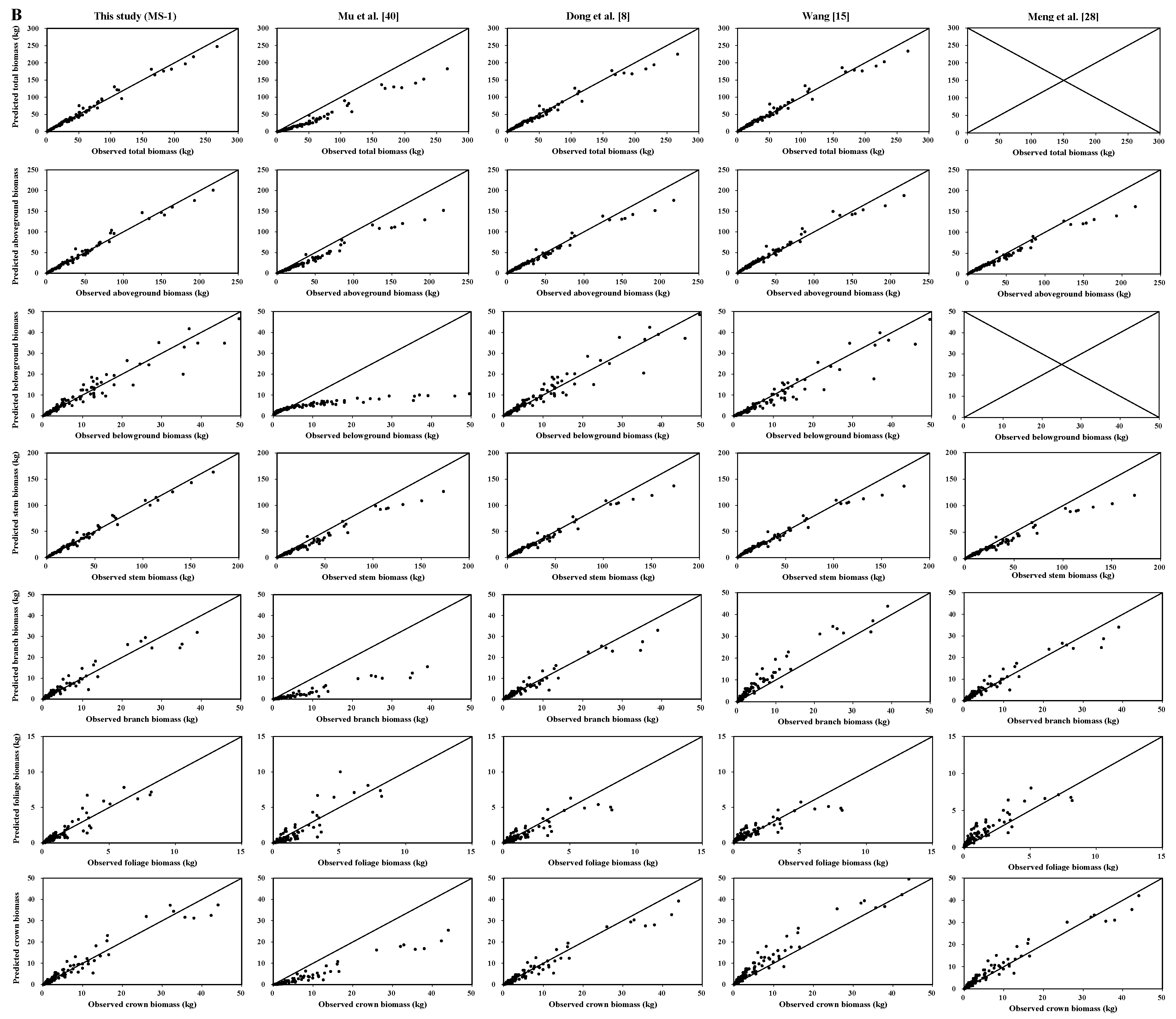
24]. Moreover, we evaluated different additive systems of biomass equations for quantifying tree- and plot-level biomass. The results indicated that, in general, the MS-1 and MS-4 performed better. However, if the variables of crown attributes are not available, MS-3 can be used to predict the total, subtotal, and component biomass of trees more accurately.
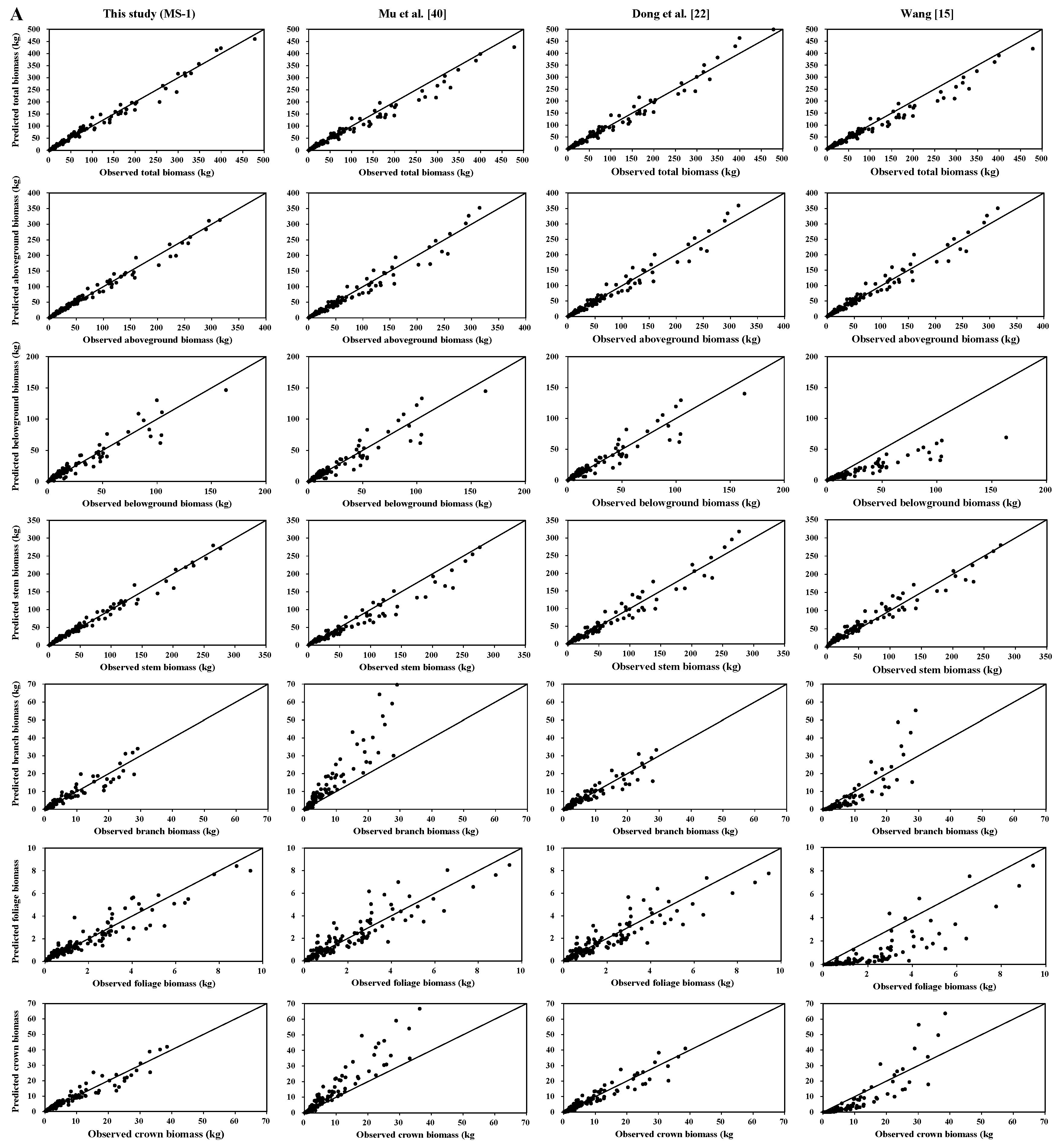
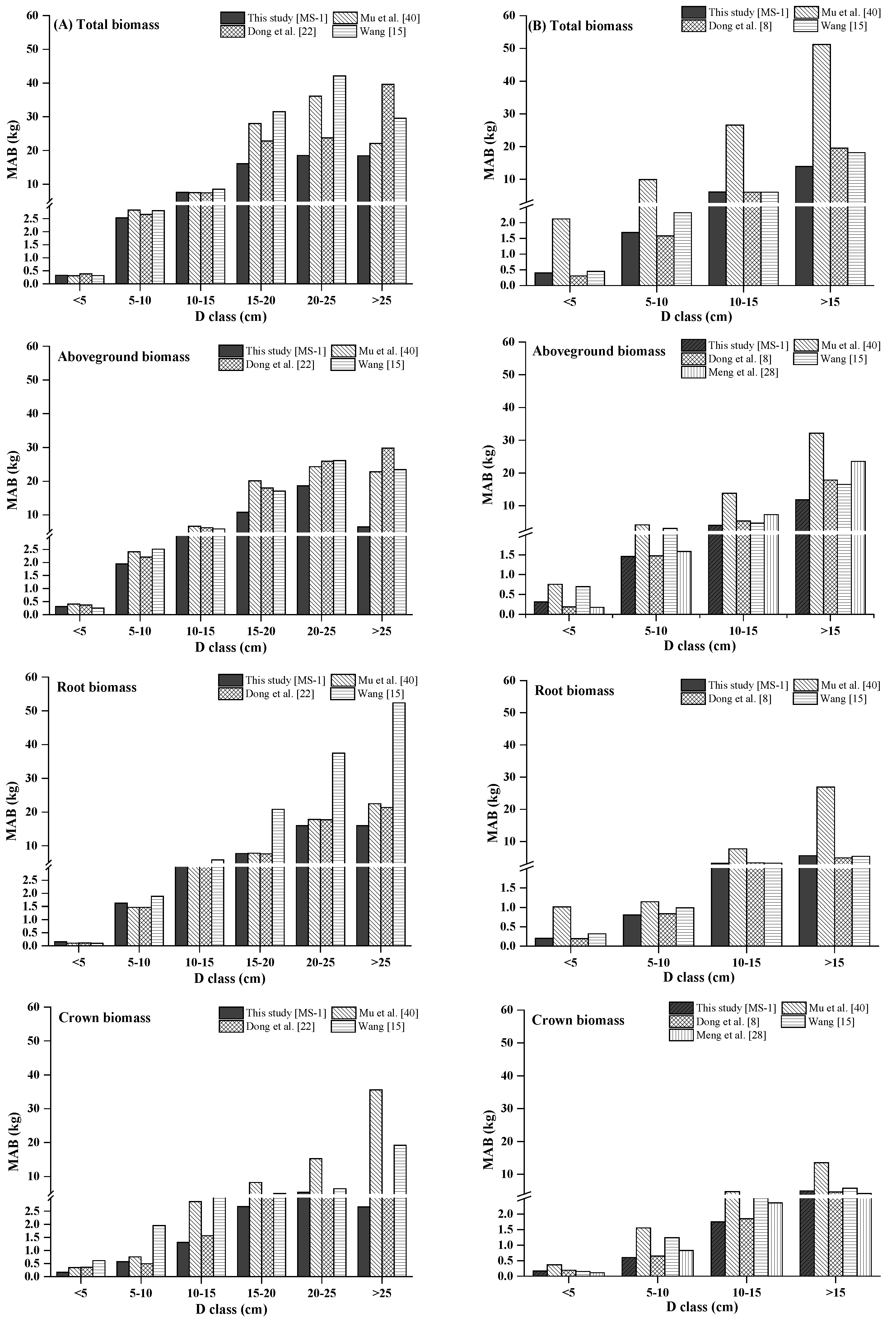
Total, aboveground, and stem biomass were better predicted than crown biomass components by our new biomass equation systems and the previously published biomass models. Our new equation systems, however, provide better prediction of each component biomass than those in the literature. Our new systems greatly improved the prediction of total, subtotal, and component biomass. There are several possible reasons: (1) the data in those four studies came from different sampling sites; (2) each species in those four studies came from different forests; and (3) the sample numbers and sample size ranges differed. These reasons could lead to differences in tree root morphological features, soil conditions, and growth processes [6,28,48,49]. Overall, the results of the graphical analysis and comparisons of MAB suggested that, for predicting biomass, our MS-1 performed better than the biomass models of Wang [15], Mu et al. [40], Dong et al. [8,22], and Meng et al. [28].
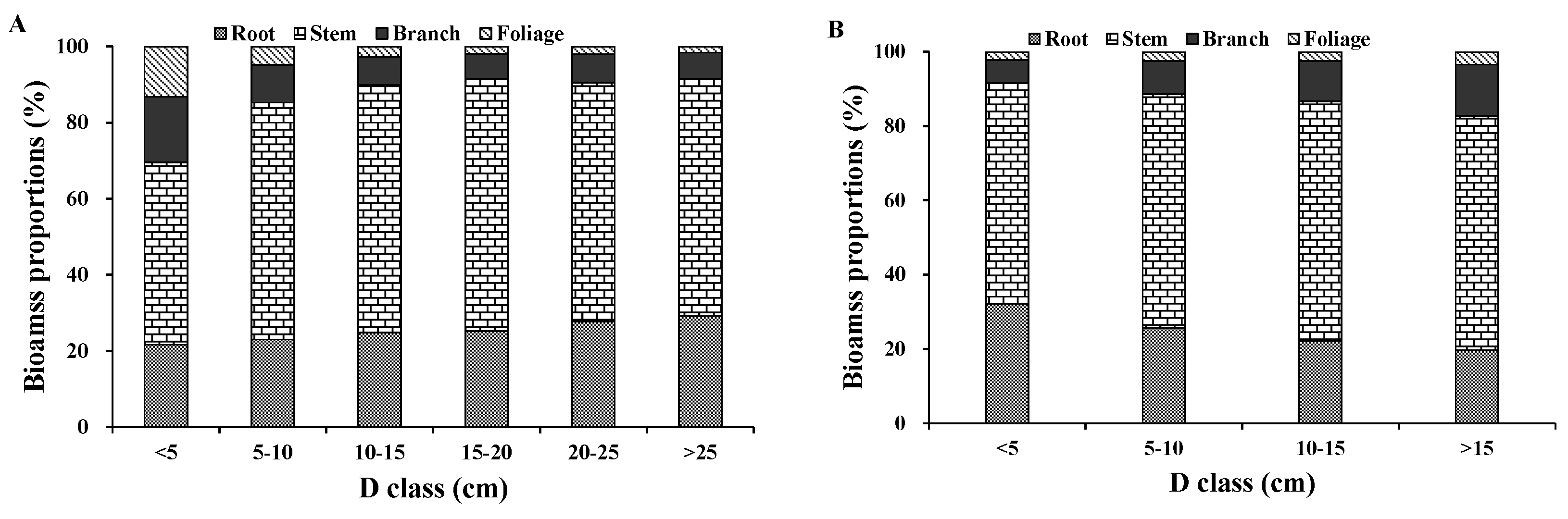
We observed a diameter-related pattern in the changes of biomass partitioning among individual aboveground tree components. For both Dahurian larch and white birch, the results demonstrated that the relative proportion of stem biomass was greater in medium- and large-diameter trees than in small-diameter trees. However, the patterns of the relative proportions of root and crown biomass were different between Dahurian larch and white birch. With respect to Dahurian larch, the crown biomass in relatively larger trees was smaller than that in relatively smaller trees, whereas for white birch, the crown biomass in relatively larger trees was greater than that in relatively smaller trees; these results occurred mostly because large white birch trees are usually forked and have thick branches, whereas Dahurian larch trees usually have a small canopy and relatively thin branches. The allocation of root biomass depends on tree root morphology (e.g., shallow root or deep root), growth processes, and soil conditions [18,50,51]. However, total root excavation was impossible for both species in this study because of the propensity of the roots to grow clonally via lateral roots. This phenomenon may introduce errors in root biomass estimation, which can then influence root biomass partitioning. The increase or decrease in root, stem, branch, and foliage biomass across different diameter classes observed in this study supports previous findings. In addition, some researchers have reported clear differences in the partitioning of different biomass components; our results showed that the aboveground biomass was approximately 75% of the total biomass, and belowground biomass was approximately 25%. Consequently, our biomass partitioning results were consistent with those in the literature [8,52,53].
Finally, because of excessive harvesting during the past 50 years, many young and middle-aged forests currently exist in the eastern Daxing’an Mountains. Thus, the sample trees from those young and middle-aged forests have relatively small D, H, CL, and CW values. Many researchers have reported that small diameters can significantly affect the estimation of total biomass. In this study, the smallest and the largest D values across both species ranged from 1.4 to 1.7 cm and from 20.5 to 28.4 cm, respectively. If the newly developed biomass equations in this study were used to estimate the biomass outside of our data range (e.g., D > 30 cm), the models could produce larger prediction errors. In addition, if our models were used in other regions, caution should be taken because different environmental and growth conditions may yield different allometric relationships between tree biomass and variables. Therefore, the biomass equations developed in this study are best suited to the eastern Daxing’an Mountains in northeast China.

5. Conclusions

In this study, four additive systems of biomass equations were developed for Dahurian larch and white birch in the eastern Daxing’an Mountains in northeast China to estimate the total, aboveground, root, stem, branch, foliage, and crown biomass. As expected, the accuracy of the biomass component equations differed among the four additive systems across both species: the model Ra2 was >0.86 for MS-1, >0.81 for MS-2, >0.81 for MS-3, and >0.84 for MS-4. The model RMSE was relatively small for the total, aboveground, and stem biomass equations, but was larger for the root, branch, foliage, and crown biomass equations. Overall, adding H and crown attributes to a system of biomass equations can significantly improve model fitting and performance.
In addition, we analyzed the biomass partitioning of the aboveground and belowground components of the two species. Our results were consistent with the literature in that stem biomass accounted for the largest proportion of total biomass. We also evaluated different additive systems of biomass equations for quantifying individual biomass. The results indicated that, in general, MS-1 and MS-4 were the best predictors of the majority of the biomass components. The overall ranking of the four additive systems of biomass equations followed the order of MS-1 > MS-4 > MS-3 > MS-2. Overall, the tree biomass data in this study was widely distributed throughout the eastern Daxing’an Mountains in northeast China. Thus, these established biomass equations can be used to estimate individual tree biomass in the Chinese National Forest Inventory. However, caution should be taken when using the newly developed systems of equations to predict biomass of trees outside the range of the data and region.

Author Contributions

L.D. participated in field work, performed data analysis, and wrote most of the paper. L.Z. helped in data analysis and wrote the paper. F.L. supervised and coordinated the research project, designed and installed the experiment, took some measurements, and contributed to writing the paper.

Acknowledgments

This study was financially supported by the Natural Science Foundation of China (31600510) and the Scientific Research Foundation for the Returned Overseas Chinese Scholars, Heilongjiang Province, China (LC2016007).

Conflicts of Interest

The authors declare no conflict of interest.

References

  1. Clark, D.A.; Brown, S.; Kicklighter, D.W.; Chambers, J.Q.; Thomlinson, J.R.; Ni, J. Measuring net primary production in forests: Concepts and field methods. Ecol. Appl. 2001, 11, 356–370. [Google Scholar] [CrossRef]
  2. González-García, M.; Hevia, A.; Majada, J.; Barrio-Anta, M. Above-ground biomass estimation at tree and stand level forshort rotation plantations of eucalyptus nitens, (Deane & Maiden) maiden in Northwest Spain. Biomass Bioenergy 2013, 54, 147–157. [Google Scholar]
  3. Konôpka, B.; Pajtík, J.; Noguchi, K.; Lukac, M. Replacing norway spruce with european beech: A comparison of biomass and net primary production patterns in young stands. For. Ecol. Manag. 2003, 302, 185–192. [Google Scholar] [CrossRef]
  4. Zeng, W.S.; Duo, H.R.; Lei, X.D.; Chen, X.Y.; Wang, X.J.; Pu, Y.; Zou, W.T. Individual tree biomass equations and growth models sensitive to climate variables for Larix, spp. in China. Eur. J. For. Res. 2017, 136, 1–17. [Google Scholar] [CrossRef]
  5. Wang, X.; Bi, H.; Ximenes, F.; Ramos, J.; Li, Y. Product and residue biomass equations for individual trees in rotation age Pinus radiata stands under three thinning regimes in New South Wales, Australia. Forests 2017, 8, 439. [Google Scholar] [CrossRef]
  6. Bi, H.; Turner, J.; Lambert, M.J. Additive biomass equations for native eucalypt forest trees of temperate Australia. Trees 2004, 18, 467–479. [Google Scholar] [CrossRef]
  7. Dong, L.; Zhang, L.; Li, F. A three-step proportional weighting system of nonlinear biomass equations. For. Sci. 2015, 61, 35–45. [Google Scholar] [CrossRef]
  8. Dong, L.; Zhang, L.; Li, F. Developing additive systems of biomass equations for nine hardwood species in Northeast China. Trees 2015, 29, 1149–1163. [Google Scholar] [CrossRef]
  9. Weiskittel, A.R.; Macfarlane, D.W.; Radtke, P.J.; Affleck, D.L.R.; Temesgen, H.; Woodall, C.W.; Westfall, J.A.; Coulston, J.W. A call to improve methods for estimating tree biomass for regional and national assessments. J. For. 2015, 113, 414–424. [Google Scholar] [CrossRef]
  10. Temesgen, H.; Affleck, D.; Poudel, K.; Gray, A.; Sessions, J. A review of the challenges and opportunities in estimating above ground forest biomass using tree-level models. Scand. J. For. Res. 2015, 30, 326–335. [Google Scholar] [CrossRef]
  11. Sileshi, G.W. A critical review of forest biomass estimation models, common mistakes and corrective measures. For. Ecol. Manag. 2014, 329, 237–254. [Google Scholar] [CrossRef]
  12. Zapatacuartas, M.; Sierra, C.A.; Alleman, L. Probability distribution of allometric coefficients and bayesian estimation of aboveground tree biomass. For. Ecol. Manag. 2012, 277, 173–179. [Google Scholar] [CrossRef]
  13. Jia, Q.Y.; Fung, T.; Ziegler, A.D. Review of allometric equations for major land covers in Se Asia: Uncertainty and implications for above- and below-ground carbon estimates. For. Ecol. Manag. 2016, 360, 323–340. [Google Scholar]
  14. Henry, M.; Picard, N.; Trotta, C.; Manlay, R.J.; Valentini, R.; Bernoux, M.; Saint-André, L. Estimating tree biomass of sub-saharan african forests: A review of available allometric equations. J. Physiol. 2011, 45, 477–569. [Google Scholar] [CrossRef]
  15. Wang, C. Biomass allometric equations for 10 co-occurring tree species in Chinese temperate forests. For. Ecol. Manag. 2006, 222, 9–16. [Google Scholar] [CrossRef]
  16. Njana, M.; Eid, T.; Zahabu, E.; Malimbwi, R. Procedures for quantification of belowground biomass of three mangrove tree species. Wetl. Ecol. Manag. 2015, 23, 749–764. [Google Scholar] [CrossRef]
  17. Mugasha, W.A.; Eid, T.; Bollandsås, O.M.; Malimbwi, R.E.; Chamshama, S.A.O.; Zahabu, E.; Katani, J.Z. Allometric models for prediction of above- and belowground biomass of trees in the miombo woodlands of Tanzania. For. Ecol. Manag. 2013, 310, 87–101. [Google Scholar] [CrossRef]
  18. Helmisaari, H.S.; Makkonen, K.; Kellomaki, S.; Valtonen, E.; Malkonen, E. Below- and above-ground biomass, production and nitrogen use in Scots pine stands in Eastern Finland. For. Ecol. Manag. 2002, 165, 317–326. [Google Scholar] [CrossRef]
  19. Huber, J.A.; May, K.; Hülsbergen, K.J. Allometric tree biomass models of various species grown in short-rotation agroforestry systems. Eur. J. For. Res. 2017, 136, 75–89. [Google Scholar] [CrossRef]
  20. Chaturvedi, R.K.; Raghubanshi, A.S. Aboveground biomass estimation of small diameter woody species of tropical dry forest. New For. 2013, 44, 509–519. [Google Scholar] [CrossRef]
  21. Daryaei, A.; Sohrabi, H. Additive biomass equations for small diameter trees of temperate mixed deciduous forests. Scand. J. For. Res. 2016, 31, 1–5. [Google Scholar] [CrossRef]
  22. Dong, L.; Zhang, L.; Li, F. A compatible system of biomass equations for three conifer species in Northeast, China. For. Ecol. Manag. 2014, 329, 306–317. [Google Scholar] [CrossRef]
  23. Kralicek, K.; Bao, H.; Poudel, K.P.; Temesgen, H.; Salas, C. Simultaneous estimation of above- and below-ground biomass in tropical forests of Viet Nam. For. Ecol. Manag. 2017, 390, 147–156. [Google Scholar] [CrossRef]
  24. Zhao, D.H.; Kane, M.; Markewitz, D.; Teskey, R.; Clutter, M. Additive tree biomass equations for Midrotation loblolly pine plantations. For. Sci. 2015, 61, 613–623. [Google Scholar] [CrossRef]
  25. Ali, A.K.; Xu, M.S.; Zhao, Y.T.; Zhang, Q.Q.; Zhou, L.L.; Yang, X.D.; Yan, E.R. Allometric biomass equations for shrub and small tree species in subtropical China. Silva Fenn. 2015, 49, 1–10. [Google Scholar] [CrossRef]
  26. Zeng, W.S. Modeling crown biomass for four Pine species in China. Forests 2015, 6, 433–449. [Google Scholar]
  27. Bi, H.; Murphy, S.; Volkova, L.; Weston, C.; Fairman, T.; Li, Y.; Law, R.; Norris, J.; Lei, X.D.; Caccamo, G. Additive biomass equations based on complete weighing of sample trees for open eucalypt forest species in South-Eastern Australia. For. Ecol. Manag. 2015, 349, 106–121. [Google Scholar] [CrossRef]
  28. Meng, S.; Liu, Q.; Zhou, G.; Jia, Q.; Zhuang, H.; Zhou, H. Aboveground tree additive biomass equations for two dominant deciduous tree species in Daxing’anling, Northernmost China. J. For. Res. 2017, 22, 233–240. [Google Scholar] [CrossRef]
  29. Zhou, X.; Brandle, J.R.; Schoeneberger, M.M.; Awada, T. Developing above-ground woody biomass equations for open-grown, multiple-stemmed tree species: Shelterbelt-grown Russian-olive. Ecol. Mod. 2007, 202, 311–323. [Google Scholar] [CrossRef]
  30. Parresol, B.R. Assessing tree and stand biomass: A review with examples and critical comparisons. For. Sci. 1999, 45, 573–593. [Google Scholar]
  31. Parresol, B.R. Additivity of nonlinear biomass equations. Can. J. For. Res. 2001, 31, 865–878. [Google Scholar] [CrossRef]
  32. Tang, S.; Li, Y.; Wang, Y. Simultaneous equations, error-in-variable models, and model integration in systems ecology. Ecol. Mod. 2001, 142, 285–294. [Google Scholar] [CrossRef]
  33. Návar, J. Biomass component equations for Latin American species and groups of species. Ann. For. Sci. 2009, 66, 208p1–208p8. [Google Scholar] [CrossRef]
  34. Russell, M.B.; Burkhart, H.E.; Amateis, R.L. Biomass partitioning in a miniature-scale loblolly pine spacing trial. Can. J. For. Res. 2009, 39, 320–329. [Google Scholar] [CrossRef]
  35. Finney, D.J. On the distribution of a variate whose logarithm is normally distributed. J. R. Stat. Soc. 1941, 7, 155–161. [Google Scholar] [CrossRef]
  36. Baskerville, G.L. Use of logarithmic regression in the estimation of plant biomass. Can. J. For. Res. 1972, 2, 49–53. [Google Scholar] [CrossRef]
  37. Clifford, D.; Cressie, N.; England, J.R.; Roxburgh, S.H.; Paul, K.I. Correction factors for unbiased, efficient estimation and prediction of biomass from log–log allometric models. For. Ecol. Manag. 2013, 310, 375–381. [Google Scholar] [CrossRef]
  38. Madgwick, H.; Satoo, T. On estimating the aboveground weights of tree stands. Ecology 1975, 56, 1446–1450. [Google Scholar] [CrossRef]
  39. Zianis, D.; Xanthopoulos, G.; Kalabokidis, K.; Kazakis, G.; Ghosn, D.; Roussou, O. Allometric equations for aboveground biomass estimation by size class for Pinus brutia Ten. trees growing in north and South Aegean islands, Greece. Eur. J. For. Res. 2011, 130, 145–160. [Google Scholar] [CrossRef]
  40. Mu, C.; Lu, H.; Wang, B.; Bao, X.; Cui, W. Short-term effects of harvesting on carbon storage of boreal larix gmelinii–carex schmidtii, forested wetlands in daxing’anling, Northeast China. For. Ecol. Manag. 2013, 293, 140–148. [Google Scholar] [CrossRef]
  41. Gong, Z.T. Chinese Soil Taxonomy; Science Press: Beijing, China, 1999; p. 615. (In Chinese) [Google Scholar]
  42. Parresol, B.R. Modeling multiplicative error variance: An example predicting tree diameter from stump dimensions in Baldcypress. For. Sci. 1993, 39, 670–679. [Google Scholar]
  43. SAS Institute Inc. SAS/ETS® 9.3. User’s Guide; SAS Institute Inc.: Cary, NC, USA, 2011. [Google Scholar]
  44. Jenkins, J.C.; Chojnacky, D.C.; Heath, L.S.; Birdsey, R.A. National-scale biomass estimators for United States tree species. For. Sci. 2003, 49, 12–35. [Google Scholar]
  45. Battulga, P.; Tsogtbaatar, J.; Dulamsuren, C.; Hauck, M. Equations for estimating the above-ground biomass of Larix sibirica in the forest-steppe of Mongolia. J. For. Res. 2013, 24, 431–437. [Google Scholar] [CrossRef]
  46. Elfving, M.B.; Ulvcrona, K.A.; Egnell, G. Biomass equations for lodgepole pine in Northern Sweden. Can. J. For. Res. 2017, 47, 89–96. [Google Scholar] [CrossRef]
  47. Lin, K.; Lyu, M.; Jiang, M.; Chen, Y.; Li, Y.; Chen, G.; Xie, J.S.; Yang, Y.S. Improved allometric equations for estimating biomass of the three Castanopsis carlesii, H. forest types in subtropical China. New For. 2017, 48, 1–21. [Google Scholar] [CrossRef]
  48. Nicoll, B.C.; Ray, D. Adaptive growth of tree root systems in response to wind action and site conditions. Tree Physiol. 1996, 16, 891–898. [Google Scholar] [CrossRef] [PubMed]
  49. Zianis, D.; Mencuccini, M. Aboveground biomass relationships for beech (Fagus moesiaca cz.) trees in Vermio Mountain, Northern Greece, and generalised equations for Fagus sp. Ann. For. Sci. 2003, 60, 439–448. [Google Scholar] [CrossRef]
  50. Strong, W.; Roi, G.L. Root-system morphology of common boreal forest trees in Alberta. Can. J. For. Res. 1983, 13, 1164–1173. [Google Scholar] [CrossRef]
  51. Canadell, J.; Jackson, R.; Ehleringer, J.; Mooney, H.; Sala, O.; Schulze, E.D. Maximum rooting depth of vegetation types at the global scale. Oecologia 1996, 108, 583–595. [Google Scholar] [CrossRef] [PubMed]
  52. Niklas, K.J.; Enquist, B.J. Canonical rules for plant biomass partitioning and annual allocation. Am. J. Bot. 2002, 89, 812–819. [Google Scholar] [CrossRef] [PubMed]
  53. Wang, J.; Zhang, C.; Xia, F.; Zhao, X.; Wu, L.; Gadow, K.V. Biomass structure and allometry of Abies nephrolepis (Maxim) in Northeast China. Silva Fenn. 2011, 45, 211–226. [Google Scholar] [CrossRef]
Figure 1. Geographical locations of the study area and sample plots in the eastern Daxing’an Mountains, northeast China.
Forests 09 00261 g001
Figure 2. Relationships between stem, root, branch, and foliage biomass and diameter at breast height (D), tree height (H), crown width (CW), and crown length (CL), respectively, for (A) Dahurian larch and (B) white birch.
Forests 09 00261 g002
Figure 3. Mean prediction error (MPE) and mean absolute error (MAE) among the total, subtotal, and component biomass for (A) Dahurian larch and (B) white birch, where RB, SB, BB, FB, CB, AB, and TB stand for root, stem, branch, foliage, crown, aboveground, and total biomass, respectively.
Forests 09 00261 g003
Figure 4. Biomass partitioning of the aboveground and belowground components of (A) Dahurian larch and (B) white birch across the 5-cm diameter (D) classes.
Forests 09 00261 g004
Figure 5. Mean absolute bias (MAB) of the four methods of estimating the individual biomass of (A) Dahurian larch and (B) white birch, where TB, AB, RB, SB, BB, FB, and CB stand for total, aboveground, root, stem, branch, foliage, and crown biomass, respectively.
Forests 09 00261 g005
Figure 6. The observed data (black dots) and model predictions from our MS-1 and the previously published biomass models for total, subtotal, and component biomass for (A) Dahurian larch and (B) white birch. The previously published biomass models include Wang [15], Mu et al. [40], Dong et al. [8,22], and Meng et al. [28].
Forests 09 00261 g006aForests 09 00261 g006b
Figure 7. Mean absolute bias (MAB) computed from our MS-1 and the previously published biomass models for total, subtotal, and component biomass across 5-cm diameter classes for (A) Dahurian larch and (B) white birch. The previously published biomass models include Wang [15], Mu et al. [40], Dong et al. [8,22], and Meng et al. [28].
Forests 09 00261 g007
Table 1. Characteristics of forest types from which the sample trees were selected. D = tree diameter at breast height; H = tree height.
Forest TypesPlotsStand Age (Years)Density (Trees·ha−1)Mean D (cm)Mean H (m)Slope (°)Altitude (m)
Dahurian larch forest1836~581240~33908.9~16.09.4~16.00~5422~960
White birch forest435~421680~21309.1~10.711.2~14.70~5480~500
Dahurian larch and white birch mixed forest931~531290~23808.7~12.611.5~14.00~5473~619
Table 2. Descriptive statistics of tree variables for the biomass data set of two tree species. CW = crown width; CL = crown length.
StatisticsDahurian Larch (N = 138)White Birch (N = 108)
MeanMinMaxSDMeanMinMaxSD
D (cm)11.01.728.46.48.41.420.54.5
H (m)11.32.421.94.910.83.121.04.0
CW (m)1.30.32.90.61.10.42.50.5
CL (m)5.01.510.51.95.71.911.52.4
Total biomass (kg)74.13 0.51 478.27 96.79 40.14 0.36 266.88 52.17
Aboveground biomass (kg)54.80 0.43 315.04 70.04 31.23 0.28 217.32 41.65
Root biomass (kg)19.33 0.08 163.24 28.09 8.91 0.08 53.19 10.91
Stem biomass (kg)47.70 0.25 276.50 61.90 25.49 0.22 173.27 33.09
Branch biomass (kg)5.35 0.11 29.10 6.99 4.59 0.05 38.99 7.34
Foliage biomass (kg)1.76 0.04 9.44 1.86 1.14 0.01 8.17 1.63
Crown biomass (kg)7.10 0.15 38.54 8.73 5.73 0.06 44.05 8.80
Table 3. Goodness-of-fit statistics of six nonlinear biomass equations based on different predictor variables for the different tree biomass components of two tree species. RMSE = root mean squared error; AIC = Akaike information criterion.
ComponentsEquationsDahurian LarchWhite Birch
Ra2RMSEAICRa2RMSEAIC
RootEquation (2) W r = β r 0 D β r 1 + ε r 0.91108.38975.30.92063.08553.1
Equation (3) W r = β r 0 ( D 2 H ) β r 1 + ε r 0.871410.071025.70.91993.09554.0
Equation (4) W r = β r 0 D β r 1 H β r 2 + ε r 0.91658.12967.40.92283.03551.0
Equation (5) W r = β r 0 D β r 1 H β r 2 C W β r 3 + ε r 0.92967.45945.00.92383.01550.6
Equation (6) W r = β r 0 D β r 1 H β r 2 CL β r 3 + ε r 0.91608.14969.30.92423.00550.0
Equation (7) W r = β r 0 D β r 1 H β r 2 CW β r 3 CL β r 4 + ε r 0.93057.41944.40.92383.01551.5
StemEquation (2) W s = β s 0 D β s 1 + ε s 0.962312.021074.20.97794.92654.7
Equation (3) W s = β s 0 ( D 2 H ) β s 1 + ε s 0.98517.57947.30.98893.48580.1
Equation (4) W s = β s 0 D β s 1 H β s 2 + ε s 0.98547.47944.70.98913.45578.8
Equation (5) W s = β s 0 D β s 1 H β s 2 CW β s 3 + ε s 0.98627.28938.70.98953.39576.1
Equation (6) W s = β s 0 D β s 1 H β s 2 C L β s 3 + ε s 0.98577.40943.00.99023.28568.8
Equation (7) W s = β s 0 D β s 1 H β s 2 C W β s 3 C L β s 4 + ε s 0.98677.14934.50.99013.29570.6
BranchEquation (2) W b = β b 0 D β b 1 + ε b 0.88432.381074.20.92232.04465.0
Equation (3) W b = β b 0 ( D 2 H ) β b 1 + ε b 0.85292.68662.90.92911.95455.1
Equation (4) W b = β b 0 D β b 1 H β b 2 + ε b 0.88952.32624.70.93091.93453.2
Equation (5) W b = β b 0 D β b 1 H β b 2 CW β b 3 + ε b 0.89142.30623.30.93051.93454.8
Equation (6) W b = β b 0 D β b 1 H β b 2 C L β b 3 + ε b 0.89872.22613.70.93141.92453.5
Equation (7) W b = β b 0 D β b 1 H β b 2 CW β b 3 CL β b 4 + ε b 0.89932.22613.90.93251.91452.7
FoliageEquation (2) W f = β f 0 D β f 1 + ε f 0.84220.74309.80.83120.67224.4
Equation (3) W f = β f 0 ( D 2 H ) β f 1 + ε f 0.79930.83342.70.81530.70234.1
Equation (4) W f = β f 0 D β f 1 H β f 2 + ε f 0.86290.69291.50.82970.67226.3
Equation (5) W f = β f 0 D β f 1 H β f 2 CW β f 3 + ε f 0.86980.67285.40.89070.54179.4
Equation (6) W f = β f 0 D β f 1 H β f 2 CL β f 3 + ε f 0.88480.63268.60.83350.83224.8
Equation (7) W f = β f 0 D β f 1 H β f 2 C W β f 3 C L β f 4 + ε f 0.88900.62264.50.89590.53175.1
The best models are given in bold.
Table 4. Model coefficient estimates, standard errors, goodness-of-fit statistics, and weight functions for the additive system of biomass equations based on the best combinations of predictors (namely MS-1). MS = model system.
Tree SpeciesBiomassβi0βi1βi2βi3βi4Ra2RMSEWeight Function
ComponentsEstimateSEEstimateSEEstimateSEEstimateSEEstimateSE
Dahurian larchRoot−3.31490.21132.36090.1476−0.02540.17090.47160.0923--0.92987.4401D3.5116CW2.5870
Stem−3.64190.07551.85730.05171.11120.05660.04710.0299−0.13030.02780.98617.2919D3.7783
Branch−3.02730.21162.67150.1495−1.16360.17960.48130.1127--0.88892.3291D5.4573H−3.1566
Foliage−2.77860.35751.86710.2765−1.04250.27950.15550.17880.72570.21900.88320.6355D2.9035
Crown----------0.90972.6225D4.7166H−2.1998
Aboveground----------0.98608.2983D5.7369H−3.2596
Total----------0.986511.2551D3.3047
White birchRoot−3.2070.14262.06060.11910.27240.1549----0.91863.1131H6.3178
Stem−3.32530.09172.18240.07220.67040.0692−0.08360.0536--0.98903.4779H4.3761
Branch−5.18720.34903.14080.167−0.24840.2501----0.91312.1622D5.2313H−3.7235
Foliage−3.66510.38212.43540.2126−0.66060.28631.44320.1165−0.33310.17530.86940.5905D11.2958H−8.7146CW2.6363CL−3.3698
Crown----------0.92972.332D5.5805H−3.6804
Aboveground----------0.98694.7685D1.1861CL2.2033
Total----------0.98636.0959D1.9543CL1.7439
Table 5. Model coefficient estimates, standard errors, goodness-of-fit statistics, and weight functions for the additive system of biomass equations based on one predictor (D only, namely MS-2).
Tree SpeciesBiomass Componentsβi0βi1Ra2RMSEWeight Function
EstimateSEEstimateSE
Dahurian larchRoot−3.81650.09742.59560.03640.91088.3896D4.6900
Stem−2.69410.07202.52490.02710.958812.5650D3.5837
Branch−3.45680.13772.01350.05160.86672.5516D2.8229
Foliage−3.21450.10611.51990.04430.81930.7905D3.3366
Crown----0.87823.0455D2.7302
Aboveground----0.968712.3884D3.9228
Total----0.978514.1805D4.0816
White birchRoot−3.09680.06872.30950.03130.92093.0685D4.0561
Stem−2.56220.02762.51500.01240.97754.9665D4.4082
Branch−5.15930.18742.86150.07220.91372.1548D3.0048
Foliage−5.56440.29592.47900.11650.83170.6703D4.4171
Crown----0.93222.2902D3.0916
Aboveground----0.97776.2132D3.4806
Total----0.97927.5328D3.7206
Table 6. Model coefficient estimates, standard errors, goodness-of-fit statistics, and weight functions for the additive system of biomass equations based on two predictors (D and H, namely MS-3).
Tree SpeciesBiomass Componentsβi0βi1βi2Ra2RMSEWeight Function
EstimateSEEstimateSEEstimateSE
Dahurian larchRoot−3.69770.26182.81290.1626−0.26710.22940.91518.1828D3.8643
Stem−3.74110.06481.83140.02971.09780.04600.98557.4496D5.7183H−2.5613
Branch−2.15090.13292.99660.1273−1.50160.16900.87552.4661D3.0179
Foliage−2.57530.14422.43880.1393−1.17850.18430.86370.6866D2.6170
Crown------0.89642.8091D3.2628
Aboveground------0.98568.4091D2.9204
Total------0.983512.4453D3.9654
White birchRoot−3.29540.11841.97180.10650.39310.13760.91913.1029H6.3178
Stem−3.40460.09522.03710.05870.77080.08600.98813.609D3.6276
Branch−5.58950.36883.10210.1442−0.08670.22980.91732.1091D5.2313H−3.7235
Foliage−3.96260.60593.09700.3496−1.20090.50050.81030.7116D4.3110
Crown------0.92942.3371D7.4044H−6.2060
Aboveground------0.98654.8324D2.8464
Total------0.98576.2395D3.0578
Table 7. Model coefficient estimates, standard errors, goodness-of-fit statistics, and weight functions for the additive system of biomass equations based on three predictors (D, H, and crown attributes, namely MS-4).
Tree SpeciesBiomass Componentsβi0βi1βi2βi3Ra2RMSEWeight Function
EstimateSEEstimateSEEstimateSEEstimateSE
Dahurian larchRoot−3.31510.21562.42830.1507−0.09320.17480.46750.09390.92947.4633D3.5116CW2.5870
Stem−3.82450.07861.70970.04721.23890.05870.04670.02760.98497.6002D3.1476CW1.2554
Branch−3.15080.22172.61940.1555−1.09310.18760.52030.11660.88992.3189D5.4573H−3.1566
Foliage−2.81360.29112.02090.2461−1.12060.28220.67170.21830.88100.6413D2.8999
Crown--------0.91022.6151D4.7166H−2.1998
Aboveground--------0.98498.5971D5.7369H−3.2596
Total--------0.985711.5701D3.3047
White birchRoot−3.31310.13131.91620.13470.33950.13230.14030.09860.91973.0923H5.9206
Stem−3.35600.09182.17210.07080.68850.0689−0.07880.05310.98913.4566H4.3761
Branch−5.26180.32792.81010.1796−0.11130.22000.26040.16760.91222.1740D4.8372H−3.1872
Foliage−3.22140.59062.81780.3623−1.36100.45390.92670.23690.84220.6489D6.7893H−3.8152
Crown--------0.92602.3926D6.3730H−4.8427
Aboveground--------0.98664.8153D1.1861CL2.2033
Total--------0.98606.1629D1.9543CL1.7439
Table 8. Comparison of different additive systems of biomass equations for individual trees of two species.
Tree SpeciesStatisticsTotal BiomassAboveground BiomassRoot BiomassStem BiomassBranch BiomassFoliage BiomassCrown Biomass
F-ValueP-ValueF-ValueP-ValueF-ValueP-ValueF-ValueP-ValueF-ValueP-ValueF-ValueP-ValueF-ValueP-Value
Dahurian larchSource of Variation
Block (tree)1820.50<0.0001790.23<0.0001676.74<0.0001429.95<0.0001162.15<0.0001109.41<0.0001152.86<0.0001
Treatment (4 MS)0.340.79800.87000.45601.410.23820.630.59910.120.94790.160.92620.030.9925
Contrasts
MS-1 vs. MS-20.000.94970.350.55592.330.12780.300.58650.210.64610.160.68730.070.7971
MS-1 vs. MS-30.000.99420.130.71930.750.38810.130.72150.310.57570.450.50440.070.7868
MS-1 vs. MS-40.710.39940.830.36270.110.74260.520.47040.080.77900.070.79220.020.8785
MS-2 vs. MS-30.000.95560.050.81840.440.50820.040.85120.010.91990.070.79080.000.9894
MS-2 vs. MS-40.610.43562.250.13423.440.06441.610.20590.030.85820.020.88930.010.9170
MS-3 vs. MS-40.700.40351.620.20451.420.23381.160.28110.080.78010.160.68590.010.9064
White birchSource of Variation
Block (tree)3769.60<0.00013173.27<0.00012626.51<0.00011604.78<0.00012056.18<0.0001111.08<0.00011026.94<0.0001
Treatment (4 MS)1.590.19123.510.01573.360.01910.980.402319.08<0.00010.200.89597.53<0.0001
Contrasts
MS-1 vs. MS-21.670.19724.200.04134.510.03451.710.19248.410.00400.010.92672.640.1053
MS-1 vs. MS-33.630.05756.660.01032.240.13550.770.382250.76<0.00010.360.551219.81<0.0001
MS-1 vs. MS-40.060.79920.010.91370.460.49910.020.87661.850.17440.000.99930.620.4323
MS-2 vs. MS-30.380.53950.280.59470.390.53130.190.666517.85<0.00010.470.49167.990.0050
MS-2 vs. MS-41.080.30023.760.05327.840.00542.140.14482.370.12500.010.92750.700.4026
MS-3 vs. MS-42.730.09956.110.01394.720.03051.060.303633.22<0.00010.360.550613.430.0003

