Article

Hydrology of Drained Peatland Forest: Numerical Experiment on the Role of Tree Stand Heterogeneity and Management

1
Department of Built Environment, Aalto University School of Engineering, FI-00076 Aalto, Finland
2
Natural Resources Institute Finland (Luke), FI-00790 Helsinki, Finland
3
Natural Resources Institute Finland (Luke), FI-90570 Oulu, Finland
4
Faculty of Science and Forestry, University of Eastern Finland, FI-80101 Joensuu, Finland
*
Author to whom correspondence should be addressed.
Forests 2018, 9(10), 645; https://doi.org/10.3390/f9100645
Submission received: 22 August 2018 / Revised: 28 September 2018 / Accepted: 12 October 2018 / Published: 16 October 2018
(This article belongs to the Section Forest Ecology and Management)

Abstract

:
A prerequisite for sustainable peatland forestry is sufficiently low water table (WT) level for profitable tree production. This requires better understanding on controls and feedbacks between tree stand and its evapotranspiration, drainage network condition, climate, and WT levels. This study explores the role of spatial tree stand distribution in the spatiotemporal distribution of WT levels and site water balance. A numerical experiment was conducted by a three-dimensional (3-D) hydrological model (FLUSH) applied to a 0.5 ha peatland forest assuming (1) spatially uniform interception and transpiration, (2) interception and transpiration scaled with spatial distributions of tree crown and root biomass, and (3) the combination of spatially scaled interception and uniform transpiration. Site water balance and WT levels were simulated for two meteorologically contrasting years. Spatial variations in transpiration were found to control WT levels even in a forest with relatively low stand stem volume (<100 m3/ha). Forest management scenarios demonstrated how stand thinning and reduced drainage efficiency raised WT levels and increased the area and duration of excessively wet conditions having potentially negative economic (reduced tree growth) and environmental (e.g., methane emissions, phosphorus mobilization) consequences. In practice, silvicultural treatment manipulating spatial stand structure should be optimized to avoid emergence of wet spots.

1. Introduction

Large-scale drainage of peatlands and paludified forests during the 1930s–1980s has remarkably increased forest growth in Finland [1] and elsewhere in the boreal region (e.g., [2,3]). In Finland, peatlands contribute to the total forest growth by about 25% [4], and drainage efficiency continues to be the key factor in the management of peatland forests [5,6].
Water balance in drained peatlands is driven by meteorological conditions and controlled by (1) drainage efficiency, (2) peat type (hydraulic conductivity and water retention properties) and peat layer thickness, (3) underlying mineral soil type, (4) stand and ground vegetation properties, and (5) site topography. Hydrological effects of peatland forest drainage have been extensively studied with experimental approaches during the past decades. However, the importance of above factors, the role of vegetation in particular, as controls of water table (WT) levels and their spatial and temporal variability, is still poorly understood.
Peatland drainage has been found to lower WT and alter runoff dynamics (e.g., [7]). Drainage efficiency (ditch spacing and depth) controls WT both directly by shortening surface and subsurface flow paths [8] and indirectly through improved tree growth and consequently increased interception and transpiration [9]. Adequate drainage in peatland forests, i.e., sufficiently low WT levels for profitable tree production, can be maintained either by regularly cleaning the ditch network, or by biological drainage through stand evapotranspiration [6]. Peat hydraulic conductivity typically decreases in deeper, more decomposed layers, reducing drainage impact on soil moisture in deeper layers compared with the more conductive surface layers. WT is also highly dependent on stand volume; in mature tree stands, evapotranspiration has been recognized as a key factor regulating growing season WT and stand growth [5,6,9], with increasing significance in the late summer [10]. Spatial variation in WT levels within a drained peatland stand was studied by Haahti et al. [11], who showed strong correlation with the distance to the nearest ditch and topography, except during a dry summer when tree proximity controlled spatial WT variations. Thus, the factors controlling WT may have different roles under different hydrologic conditions, which complicate their empirical analysis. Variations in WT levels in drained peatland forests are also linked to nutrient export to water courses [12], mercury methylation [13], and greenhouse gas balance [14], which makes understanding the controls of WT levels important in a wider context.
Interest towards continuous-cover forestry has grown in recent years because it is considered more environmentally and societally sustainable compared to even-aged forestry [15,16]. Replacing clear-cutting with alternative harvesting methods such as canopy gap cuttings and selective removal of trees further increases the need to understand the role of vegetation on WT levels. In particular, the more heterogeneous vegetation cover is likely to increase spatial variation of evaporation and transpiration and thereby affect spatial and temporal WT distributions in drained peatland forests.
Various modeling studies have been conducted in drained peatland forests to quantify runoff generation, water balance, and WT dynamics across a range of weather conditions and drainage configurations. These include one-dimensional (1-D) models such as DRAINMOD-FOREST [17,18] and the CoupModel [19], and quasi-two-dimensional FEMMA model which has been widely applied in Finland [20,21,22,23]. Three-dimensional (3-D) distributed hydrological modeling in drained peatlands has been conducted with GEOtop [24] and FLUSH models [25]. While some of the model applications have embedded a spatial description of the peatland, the effect of spatially varying stand characteristics and evapotranspiration has not been considered in earlier studies. Physically-based 3-D hydrological models, such as FLUSH [25,26], are among the most promising tools to analyze spatial differences of soil moisture, WT levels and water balance within a drained peatland. We expect that such modeling can significantly increase the understanding of the effect of heterogeneous vegetation on spatial and temporal variability of WT levels. This would further enable the simulation of different harvest regimes in their ability to sustain sufficient drainage for tree growth.
In hydrological models, the stand characteristics are conventionally described using average stand values, such as dominant height, basal area and stand volume, which disregard any spatial information of individual trees. The tree stand structure on drained peatlands is clearly uneven [27,28,29], which suggests considerable spatial differences in transpiration and interception capacity within the tree stand that should be considered in hydrological modeling. Spatially averaged stand properties may be sufficient for modeling average water balance components but methodological development is needed to assess the spatial variability of hydrological state variables, such as WT. First steps towards spatially advanced hydrological modeling should therefore include accounting for the spatial heterogeneity in tree stand interception and transpiration. This is timely since terrestrial and airborne laser scanning [30,31] are already able to provide necessary information on spatial stand heterogeneity to be incorporated into ecohydrological models.
The objective of this study was to evaluate the role of spatial stand characteristics and the ditch network in the spatiotemporal distribution of WT levels and water balance of a drained peatland forest. To address these questions, a numerical experiment was carried out utilizing a process-based distributed hydrological model [26], offline-coupled with a simple vegetation ecohydrological model, during two meteorologically contrasting growing seasons in a 0.5-ha peatland forest, where WT had been observed from 50 tubes [11]. The aim of the numerical experiment was (1) to test the hypothesis that spatial variation in interception and transpiration within the tree stand would cause significant spatiotemporal variation in WT depths, and (2) to test how forest management may affect WT depths on a drained peatland.

2. Materials and Methods

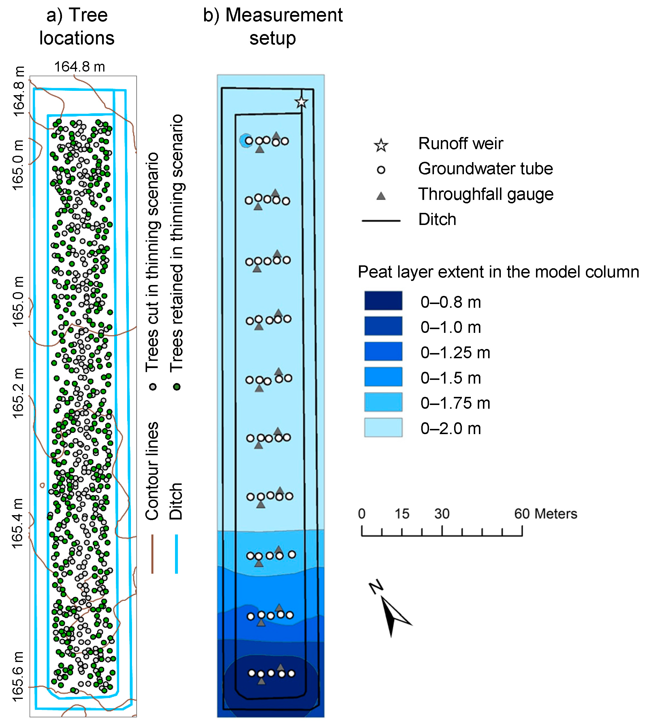
2.1. Sattasuo Experimental Area and Measurements

Sattasuo is an open-ditch-drained peatland forest area in Rovaniemi (66°30′ N, 26°42′ E), northern Finland. Climate in the region is characterized by a 30-year (1981–2010) average air temperature of 0.6 °C (with −11.7 °C in February and 15.0 °C in July) and average precipitation of 505 mm a−1 [32]. Snow typically covers the ground from October to May. The area was first drained in 1934 followed by ditch cleaning in 1985. For research purposes, a 0.5-ha forest strip was isolated from its surroundings by double ditching in 2006 which included the second cleaning of the existing ditches (Figure 1a). The average stand volume in 2006 was 93 m3 ha−1 with Scots pine (Pinus sylvestris L.) as the dominant tree species (98% of volume). The location, species, and diameter at breast height (DBH) of individual trees were measured and mapped manually based on distance and direction from mapping points (Figure 1a) in 2006.
Within the stand area, 50 groundwater tubes were installed (Figure 1b) and peat layer thickness was measured next to each tube. Utilizing that data, peat layer thickness was interpolated over the area. The peat layer thickness extended beyond the ditch depth, except for the southern end of the area (Figure 1b). According to the Finnish site type classification [33], Sattasuo represents a medium productivity site. The ground vegetation was composed of a 0.3–0.5 m high layer of dwarf shrubs (Rhododendron tomentosum Harmaja, Vaccinium uliginosum L., and Betula nana L.). The topography of the area is flat with average slope 0.2°. A digital elevation model (DEM) was constructed for the area from openly available Lidar data [34] by first creating a 10 × 10 m2 DEM which was then interpolated to a 1 × 1 m2 grid.
WT depths (the distance between the soil surface and the WT level) were manually measured from 50 groundwater tubes (Figure 1b) at 1–2 week intervals during the unfrozen season (May to October) in 2006 and 2007. The length of the tubes below the soil surface, and thus the maximum measurement depth of WT, was 1 m. Throughfall under the overstory canopy was measured in 2007 using 20 precipitation gauges (Figure 1b) emptied at least once a week during June–September. Sapflow measured from seven trees at 10-min intervals provided an estimate for the stand-average transpiration (see Figure A1). The sapflow measurements were based on the Granier method [35]. Trees for the measurements were selected to represent dominant and co-dominant pines located at different distances from ditch in the middle of the peatland strip. Sapflow tree diameters ranged from 127 to 174 mm. In this study, the role of the experimental site and the measurements was not to characterize a specific drained peatland forest area for hydrological modeling of drainage conditions (i.e., the model was not systematically calibrated), but the observational data was used to ensure that the model produces realistic WT depths on a typical drained peatland forest.

2.2. 3-D Distributed Hydrological Model FLUSH

To simulate water balance components and the spatiotemporal variability of WT, the hydrological model FLUSH [36] was applied together with a simple vegetation ecohydrological model [37]. FLUSH is a distributed, open-source 3-D hydrological model originally developed for subsurface drained agricultural fields, and recently applied also to an open-ditch-drained peatland forest site [25]. In FLUSH, overland flow is simulated in 2-D with the diffusive wave approximation of the St. Venant equations and 3-D subsurface flow with the numerical finite volume solution of the Richards equation. The subsurface domain in FLUSH comprises soil matrix and macropore systems, but only a single pore (soil matrix) system was considered in this study. FLUSH applies the Mualem-van Genuchten schemes [38] to quantify water retention and unsaturated hydraulic conductivity in the soil. Ditches act as sinks in the overland and subsurface domains (see [25]). Water in the root zone can be removed by transpiration, which is determined in FLUSH using input time series of potential transpiration (transpiration rate without soil water constraints), the root mass distribution, and the soil moisture conditions. The restriction of transpiration during inadequate soil moisture supply was described according to the scheme presented by Lagergren and Lindroth [39].
In this study, FLUSH was modified to feed in spatially varying throughfall (Fpot) and tree stand transpiration (Epot,o), and separate Epot,o and potential understory transpiration (Epot,u). Time series of these input variables were computed off-line using the simple vegetation ecohydrological model detailed in Section 2.4 and Appendix A.1, Appendix A.2 and Appendix A.3.

2.3. Discretization and Parameterization

The modeled area (0.6 ha) was outlined by the inner ditch network (see Figure 1a). The ditches were prescribed with a depth of 0.95 m and a constant water depth of 0.1 m. The size of the soil columns used in the FLUSH simulations were 2 × 2 × 2 m3. Each soil column was vertically discretized to 18 calculation cells; 0.05 m thick layers down to the depth of 0.4 m, then 0.1 m layers down to 1 m depth, and finally 0.25 m layers down to 2 m depth. The depth of the root zone was set to 0.2 m. The peat hydraulic properties (Table 1) were based on a previous study in the same area [21]. In that study, the water retention curve parameters for the layers 0–0.2 m were adopted from Päivänen [40] and the parameters for the deeper layers from soil sample analysis. Vertical saturated hydraulic conductivities of peat (KVsat) for layers 0.2–2.0 m were set based on Päivänen [40] and for layers 0–0.2 m manually adjusted comparing the simulated WT depths against measured WT depths. Saturated horizontal hydraulic conductivities (KHsat) were set to 10 × KVsat in layers at depths 0–0.6 m and equal to KVsat in deeper layers (for anisotropy of peat hydraulic conductivity, see e.g., [41,42]). The depth of the peat layer within the model area was described according to Figure 1b. The underlying mineral soil was characterized as silt loam and the parameters adopted from Vakkilainen [43].

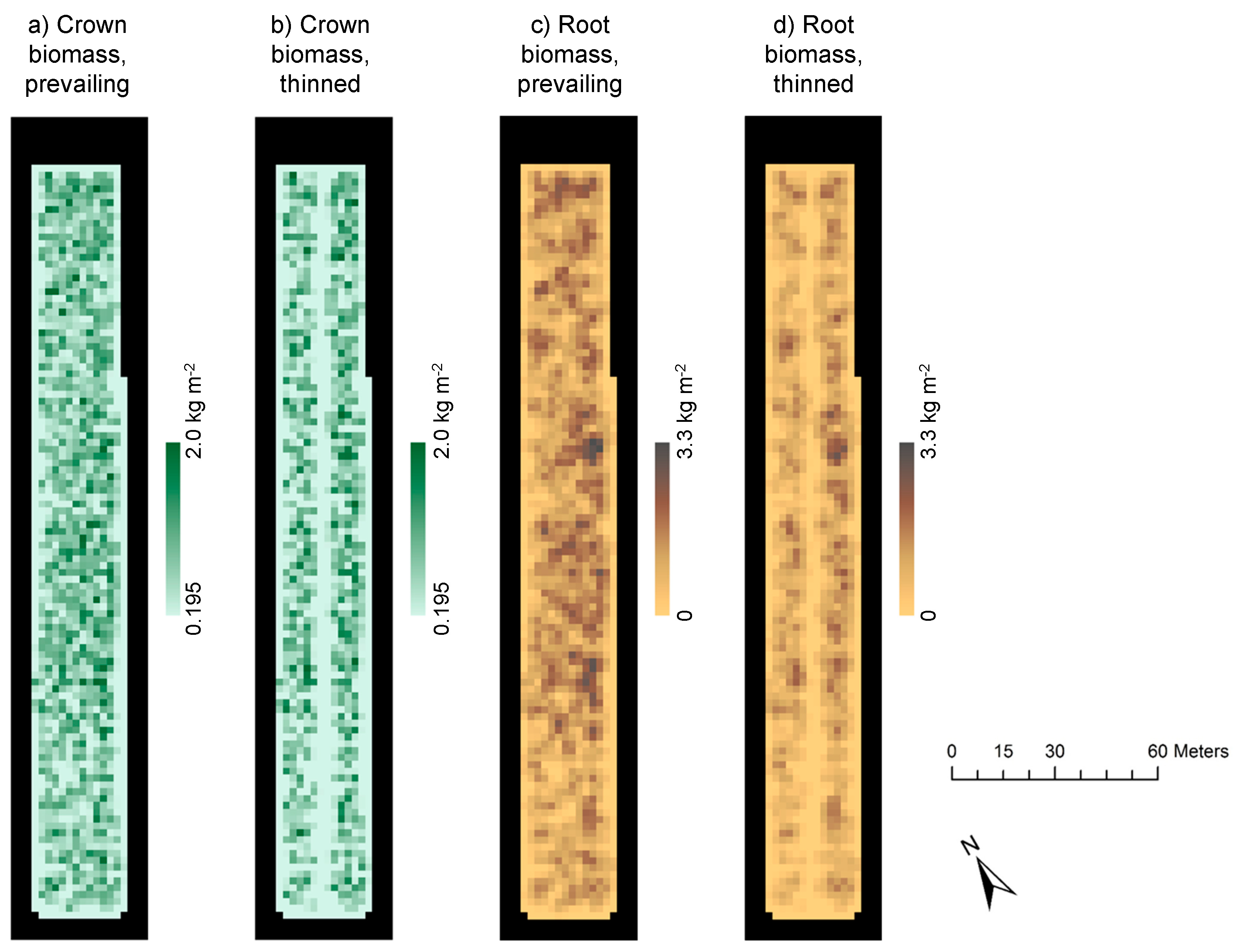
2.4. Computing and Spatial Scaling of Inputs for the FLUSH Model

The FLUSH model requires potential transpiration and throughfall to soil surface as inputs. Stand-average interception rate (Iav) and potential transpiration rates (Epot,av) were estimated using a simple vegetation ecohydrological model [37] forced by daily meteorological data provided for Finland at a 10 × 10 km2 resolution by the Finnish Meteorological Institute (FMI). The computed interception accounted for water intercepted by the overstory canopy and by the field (shrubs) and bottom (living moss) layers (see Appendix A.1). Potential transpiration rates were computed for the overstory and understory assuming that both layers are well coupled to the atmosphere:
E p o t , i ,   a v = G i D v p P a m b
where Epot,i,av (mm d−1) is the stand-average potential transpiration rate of layer i (for overstory (o) or understory (u)), and Dvp and Pamb are the vapor pressure deficit and the ambient pressure (kPa), respectively. The daily canopy conductance Gi (mm d−1) was computed accounting for the effect of the photosynthetically active radiation, the leaf-area index of layer i (LAI, m2 m−2), Dvp and the seasonal cycle of vegetation (see Appendix A.3). The parameter values of both interception and Gi models were initially derived, and the predictions evaluated against measurements from a Scots pine forest at Hyytiälä, Southern Finland and at eight additional boreal sites. Here the model predictability was checked by comparing the predicted throughfall rate (below overstory canopy) and overstory transpiration rate against the spatially averaged throughfall and sapflow measurements, respectively (see Figure A1). Note that Epot computed by the simple vegetation ecohydrological model is actual transpiration rate without possible soil moisture limitations that were subsequently accounted for within the FLUSH.
The spatial distributions of tree biomass (crown and root) were used to describe spatially variable potential overstory transpiration and throughfall. The biomass distributions were generated as 2 × 2 m2 rasters based on the point locations and DBH of the trees (Figure 1a). First, the biomasses of individual trees were calculated using the DBH data and applying the biomass equations by Marklund [44]. Crown and root projection areas were then determined for each tree [45,46], and biomasses assumed to be evenly distributed over the projection area of the tree. The resulting biomass rasters for the prevailing and the retained (see Section 2.5) tree stand are shown in Figure 2. The average crown biomasses (and their standard deviation) in the area were 0.39 (0.36) and 0.23 (0.29) kg m−2 for the prevailing and retained tree stands, respectively, and the average root biomasses 0.97 (0.65) and 0.63 (0.54) kg m−2.
The crown biomass distribution was used to estimate the spatial distribution of interception. The measurements indicated that the observed cumulative throughfall correlated well with the crown biomass within 2 m radius of the precipitation gauge (correlation −0.61 in 2007). Thus, stand-average interception was scaled linearly based on the crown biomass distribution. Throughfall to soil surface at a grid cell j (Fpot,j) was obtained by:
F p o t , j = P c j I a v
where P is precipitation and cj is a scaling coefficient proportional to the crown biomass in cell j. The coefficient cj was calculated to fulfill that (1) Fpot,j is positive and that (2) the average of interception of individual cells equals Iav (see Appendix A.2).
The root biomass distribution was used for the linear scaling of stand-average overstory transpiration. Potential overstory transpiration at a grid cell j (Epot,o,j) was calculated by:
E p o t , o , j = b r o o t ,   j b r o o t , a v E p o t , o , a v
where broot is the tree root biomass, broot,av is the stand-average tree root biomass, and Epot,o,av is the stand-average potential overstory transpiration.

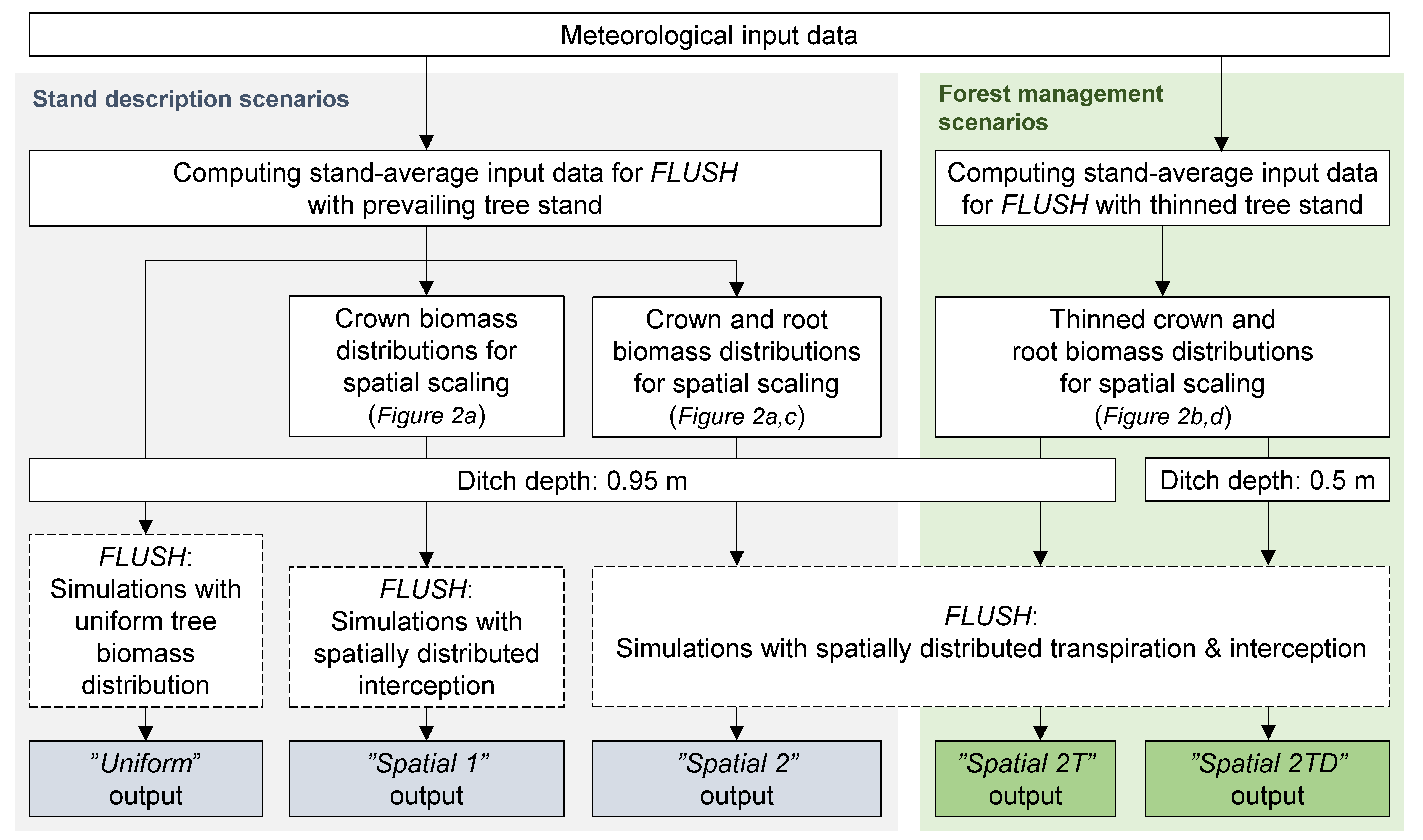
2.5. Model Scenarios

Model scenarios (Figure 3) were divided to (1) stand description scenarios that were utilized in model development, and (2) forest management scenarios. In the three stand description scenarios, FLUSH was applied to test the effect of spatially varying interception and transpiration rates on site water balance and WT levels. In the forest management scenarios, the effect of thinning of the stand and the impact of varying ditch depth on water balance and WT levels were examined. FLUSH simulations utilized the same soil parameterization in all scenarios. FLUSH was applied for a two-year-period (2006–2007) using a time step of one hour. The meteorological data were compiled from the gridded daily precipitation provided by FMI, Apukka weather station operated by FMI, and locally recorded weather station data. The local data were from a nearby open field weather station (operated by Natural Resources Institute Finland), where hourly air temperature, relative humidity, and wind speed were available. When hourly input data were not available, the daily input time series (see Section 2.4) were divided uniformly to 24 h.
The Uniform scenario used spatially uniform interception and potential transpiration and thus corresponded to model parameterization using traditional, site-averaged, forest mensuration approach. Consequently, it provided an analysis of the impact of drainage design, topography, and soil properties on the spatial distribution of WT levels. The Spatial 1 scenario was similar to the Uniform scenario except that interception was scaled according to the crown biomass distribution (Equation (2), Figure 2a). In the Spatial 2 scenario, both the interception and overstory potential transpiration were scaled based on tree biomass distributions (Equation (3), Figure 2a,c). By comparing the results of Spatial 1 and Uniform scenarios, we aimed to address the effect of spatial variability of interception on WT depths. Comparing the Spatial 1 and Spatial 2 scenarios was assumed to reveal the impact of spatial transpiration variation on WT depths.
The two forest management scenarios were applied by modifying the Spatial 2 scenario with thinning of the tree stand (Figure 1a and Figure 2b,d) (Spatial 2T) and ditches with poor water conducting capacity (Spatial 2TD). In the Spatial 2T scenario about one third of the trees were cut, removing primarily the smallest trees. All trees were removed from a haulage trail (width of 5 m) located midway between the ditches. Such treatment represents the typical first commercial thinning of drained peatland pine stands. Finally, Spatial 2T scenario was modified by reducing ditch depth to 0.5 m to simulate the conditions after thinning in the case of a ditch network with reduced drainage efficiency (scenario Spatial 2TD, Figure 3).

3. Results

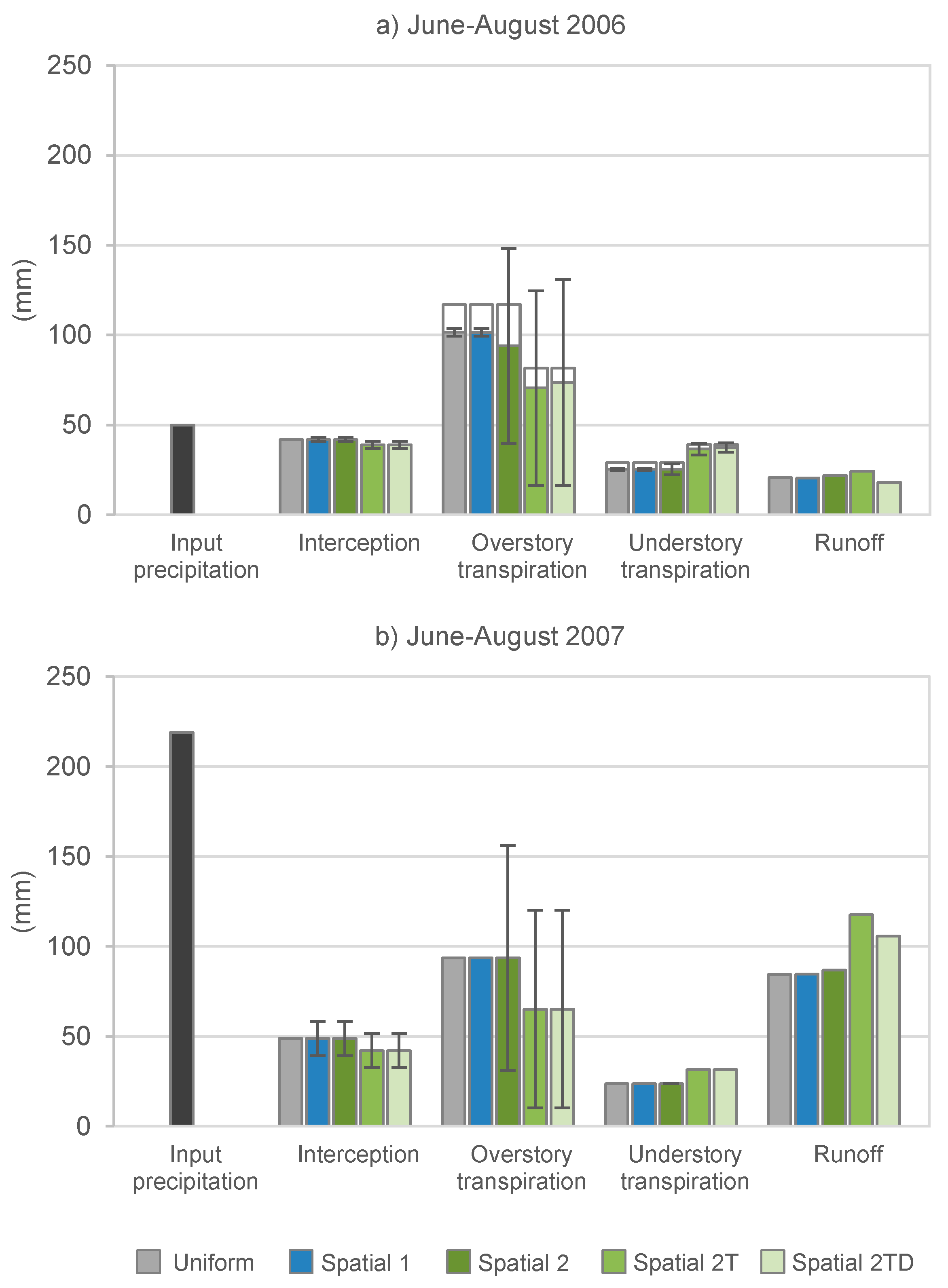
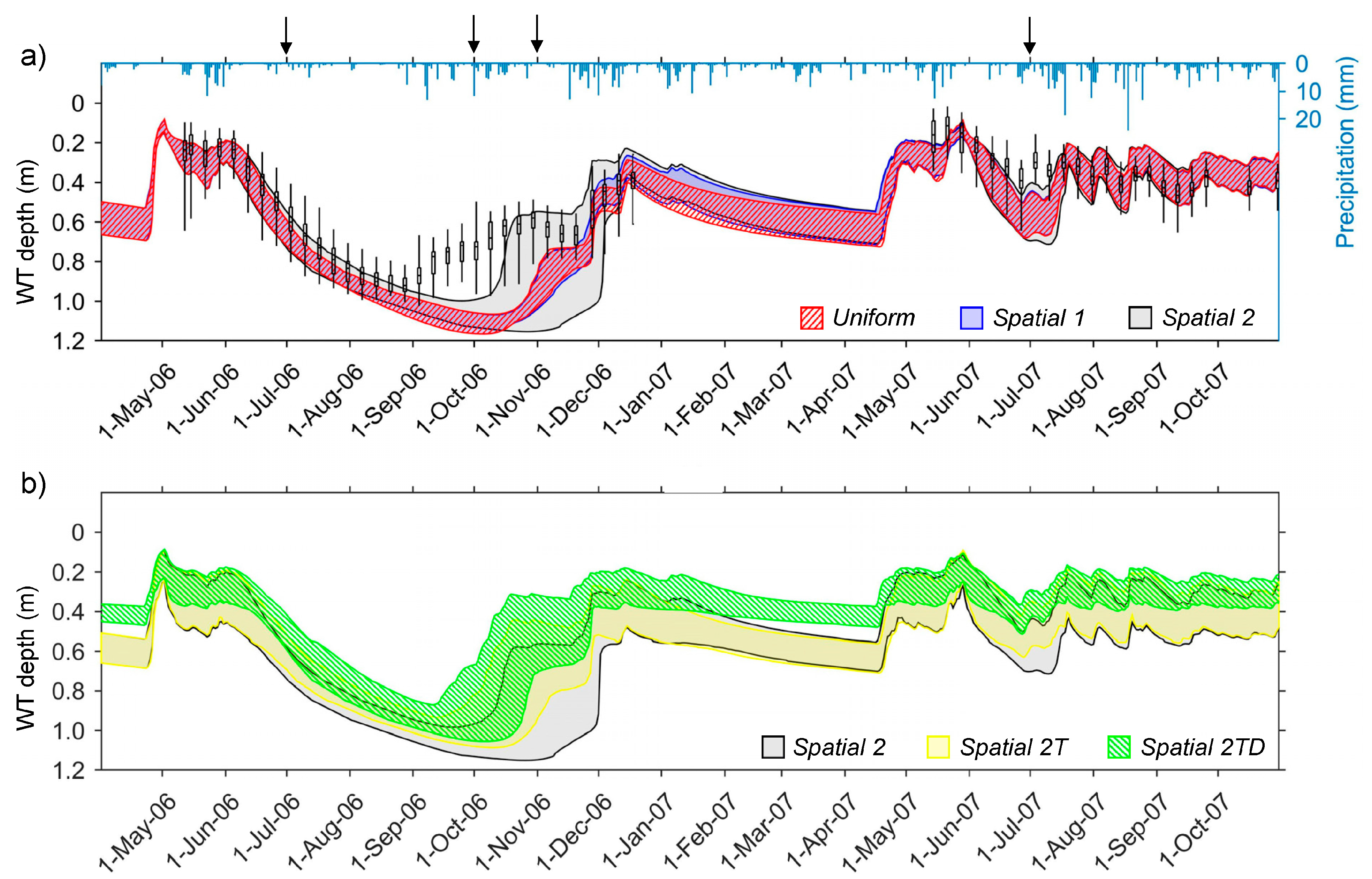
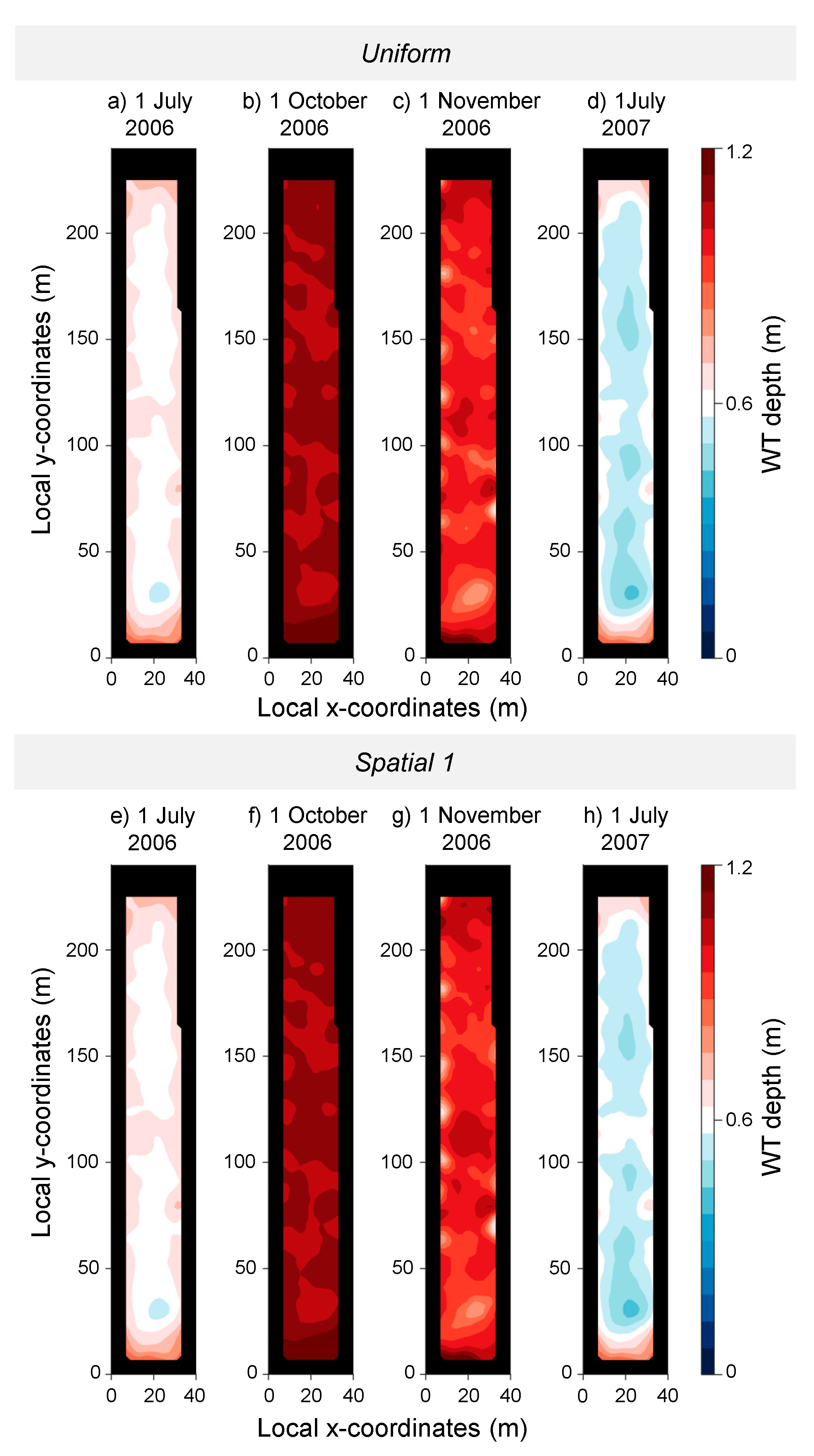
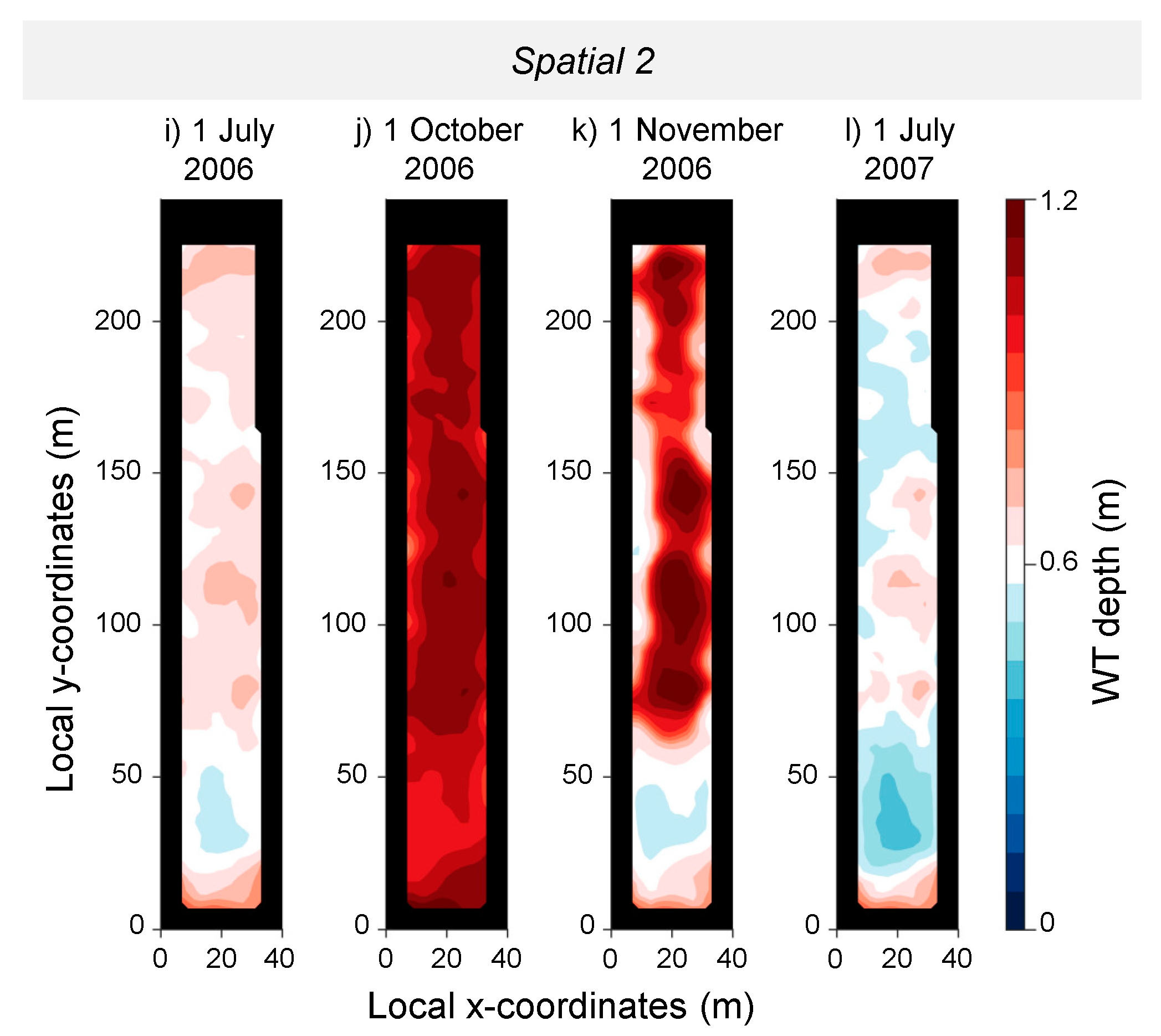
3.1. Stand Description Scenarios: The Role of Spatially Distributed Interception and Transpiration in Water Balance and WT Levels

The peatland water balance was strongly controlled by weather conditions during the two contrasting summers. Summer (June–August) 2006 was dry with only 50 mm of precipitation whereas the summer of 2007 was typical with 219 mm of precipitation (Figure 4). The large difference in precipitation was most clearly reflected to runoff volumes. Summer 2006 was slightly warmer than 2007; daily average temperatures between June–August were 14.8 °C in 2006 and 13.7 °C in 2007. The nearly similar level of available summer season energy (in terms of temperature) was seen as a minor difference between the evapotranspiration components.
The computed stand-average water balance components were mostly similar among the stand description scenarios (Uniform, Spatial 1 and Spatial 2) (Figure 4). The main difference between these scenarios was that the stand-average overstory transpiration was lower (by 8 mm) in 2006 in the Spatial 2 scenario than in the Uniform and Spatial 1 scenarios. Compared to the potential overstory transpiration (calculated as in Section 2.4), the simulated overstory transpiration was in the dry 2006 growing season limited by reduced water availability in the root zone in all stand description scenarios, by 13% in the Uniform and Spatial 1 scenarios and by 20% in the Spatial 2 scenario. In the summer of 2007, the overstory and understory transpiration were equal to their potential rates in all stand description scenarios. Spatial variability of modeled interception was higher in the moister 2007 than in the dry 2006 (Figure 4). The share of interception from precipitation was clearly greater in 2006 than in 2007. There were minor differences in runoff between the Uniform, Spatial 1, and Spatial 2 scenarios (Figure 4).
The modeled WT followed a similar pattern as measured WT, with lower levels during the dry summer of 2006 and higher levels during the wet summer of 2007 (Figure 5a). The Spatial 1 scenario with spatially scaled interception did not deviate much from the Uniform scenario. The Spatial 2 scenario with spatially scaled interception and transpiration, however, showed clearly higher spatial variability in WT depths in October–November 2006 than the other two stand description scenarios (Figure 5a). A less pronounced but similar effect was noted also in July 2007. During June–July 2006, the WTs modeled with the Spatial 2 scenario corresponded well with the variation in the measured values, but during the following autumn the modeled spatial variation clearly exceeded the measured spatial variation (Figure 5a). Autumn rainfalls after the dry summer in 2006 caused a rise in the measured WT in September, while the modeled WT levels did not rise until in October.
Simulated WT depths are shown for four summer and autumn dates in Figure 6 and highlight the clear temporal differences but reveal no notable spatial differences between the Uniform (Figure 6a–d) and Spatial 1 (Figure 6e–h) scenarios. The impact of drainage ditches on WT can be detected by lower WT levels at forest edges in July when WT is not as deep as in October and November. The Spatial 2 scenario differs clearly from the other two scenarios and demonstrates how spatial transpiration variability has stronger impact on spatial WT distribution than does the interception variability. Especially in November 2006, the WT depths have clearly larger spatial variation in the Spatial 2 scenario than Spatial 1 scenario (Figure 6k). The wet area in the southern part, and the dryer areas in middle parts are more pronounced in the Spatial 2 scenario (Figure 6i,k,l) compared to the Uniform and Spatial 1 scenarios.

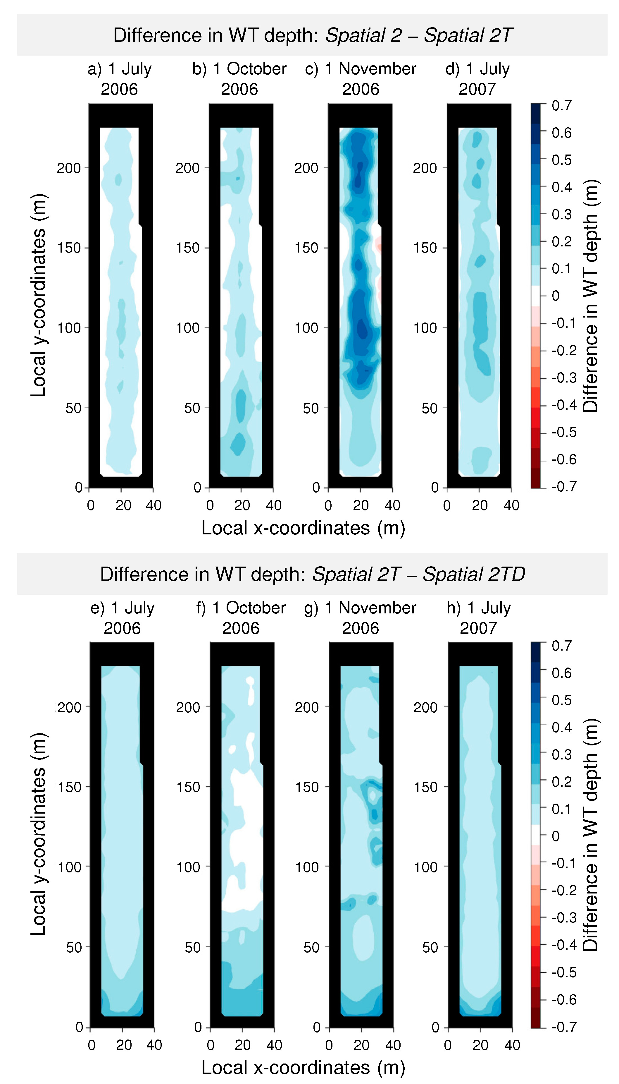
3.2. Forest Management Scenarios: The Effects of Forest Management on WT Levels

Thinning of the tree stand in the Spatial 2T scenario (see Section 2.5 and Figure 1a) resulted in higher WT compared to the prevailing tree stand in the Spatial 2 scenario (Figure 5b): The WT levels were on average 0.04 or 0.06 m higher during June–August 2006 and 2007, respectively. The greatest differences were noted in October–November 2006, probably because of faster WT rise after the autumn rainfalls in the thinned stand (Figure 5b). In addition, WT was clearly higher in July 2007 in the thinned Spatial 2T scenario than in the prevailing (Spatial 2) tree stand (Figure 5b). The highest WT levels were found in the Spatial 2TD scenario with thinned tree stand and reduced drainage efficiency (Figure 5b). On average, WT levels were 0.07 m higher in Spatial 2TD scenario compared to the Spatial 2T scenario during June–August in both 2006 and 2007. Spatial 2TD scenario also resulted in smaller spatial variation in the WT levels than Spatial 2T in 2007 (Figure 5b).
The results showed that WT was elevated in the Spatial 2T scenario especially in the middle of the area representing the haulage trail (Figure 7a–d). Reduced drainage efficiency in Spatial 2TD scenario inflicted a rather uniform rise in WT during both summers (Figure 7e,h), but in autumn 2006 the rise was less systematic (Figure 7f,g). Examination of the WT depths in 2007 revealed that the time when more than half of the area suffered from excess moisture (here assumed WT depth < 0.3 m, see [47]) during the period critical for root growth (July–August, see [48]) clearly increased due to thinning (Spatial 2T) and increased even more due to the combination of thinning and reduced drainage efficiency (Spatial 2TD) (Table 2).
In the thinned stand there was a small decrease in the average interception, clear decrease in the average overstory transpiration, and a small increase in the average understory transpiration compared to the prevailing tree stand (Figure 4). Even though the average overstory transpiration decreased due to thinning, its spatial standard deviation was about the same (54–57 mm) in Spatial 2, Spatial 2T, and Spatial 2TD scenarios in 2006. In 2007, the standard deviation was higher in Spatial 2 (63 mm) than in Spatial 2T and Spatial 2TD scenarios (55 mm). Compared to the potential overstory transpiration, the simulated overstory transpiration was limited by dry conditions in 2006 on average by 14% and 10% in Spatial 2T and Spatial 2TD scenarios, respectively. Thinning (Spatial 2 compared to Spatial 2T) clearly increased runoff (+31 mm) in the wet summer of 2007 but not much (+2 mm) in the dry summer of 2006 (Figure 4). Compared to Spatial 2T scenario, reduced drainage efficiency in Spatial 2TD scenario decreased runoff by 6 and 12 mm in the dry and wet summers, respectively. The difference in runoff between Spatial 2T and Spatial 2TD scenarios was mostly due to longer recession of spring snowmelt runoff in Spatial 2T scenario.

4. Discussion

It is obvious that spatially distributed hydrological modeling that considers tree distribution of a forest improves the prospects of identifying the spatial patterns of soil moisture, which can exert strong controls on tree growth, biogeochemistry and greenhouse gas balance of drained peatlands. In dry conditions, organic matter decomposition and nutrient release can be restricted (e.g., [49]), decreasing tree photosynthesis and productivity. On the other hand, excessively wet areas in drained peat soils are prone to disturbed root growth, increased methane emissions [14], phosphorus leaching [12] and mercury methylation [13]. This study provided the first steps towards acknowledging the spatial stand distribution in hydrological modeling of drained peatlands.
The Uniform and Spatial 1 (spatially variable interception) scenarios resulted in similar WT levels (Figure 5a), indicating that the spatial distribution of interception had minor effects on WT levels. On the other hand, the Spatial 2 scenario demonstrated that spatial distribution of transpiration had a strong impact on the variation of WT levels, particularly during dry periods. High spatial variation in transpiration even resulted in local drought stress, which was suggested by the model simulations during the dry summer. In the Spatial 2 scenario with spatially scaled transpiration and interception, the spatial variations in WT depths were striking, in spite of the relatively low-stocked tree stand. In forests with higher biomass, the tree stand plausibly exerts an even significantly stronger control on WT levels than demonstrated in this study. Denser tree stands reflect directly to interception [50,51,52,53], transpiration [54,55,56], root channel macropores, and snow accumulation within the stand [51].
The spatial distribution of ground vegetation transpiration was not considered in this study. It is, however, likely that in reality the ground vegetation partly compensates for the lack of overstory transpiration in canopy openings, as well as in sparsely stocked forests. In mature dense forests, however, radiation is primarily available for evaporation and transpiration of the tree stand. In such conditions the transpiration of the shaded ground vegetation is minor. In future, it is important to better understand the role of understory on site water balance, in particular in peatland forests with abundant shrub vegetation, where understory vegetation evapotranspiration may amount to as much as that of the tree stand [6].
The model could not correctly predict the timing of WT level rise after the dry summer (Figure 5a). This may be due to overestimation of evapotranspiration demand during growing season, which can lead to an underestimation of WT response to subsequent rainfalls. Most likely, however, the model bias is related to the single pore system description in the model (i.e., no preferential flow paths), which during dry conditions results in poorly conductive surface peat layers that prevent infiltration to the deeper layers at the onset of rainfalls. The instant WT level rise observed at Sattasuo after rainfall on dry soil is probably caused by preferential flow paths [57], and simulating their impact on infiltration and soil water redistribution is an additional need for modeling the drained peatland hydrology.
The period July–August has been suggested as the most critical season for Scots pine roots growth [48] and thus it was examined closer in our study. Our numerical experiments on forest management (thinning with reduced drainage efficiency, i.e., Spatial 2TD scenario) suggest that cleaning (i.e., deepening) the ditch network would have been beneficial in Sattasuo in connection with the first commercial thinning to avoid excess wetness. On the other hand, larger tree stands than in Sattasuo are likely to maintain the WT levels at sufficient depth through evapotranspiration [5,6], and ditch cleaning may be unnecessary even with ditches with poor drainage efficiency.
Our results indicated that thinning of the tree stand raised WT levels especially in the haulage trail. Such a result can have negative environmental consequences because soil compaction at the wheel ruts decreases hydraulic conductivity and reduces the quantity of macropores [58]. Such circumstances can create anoxic conditions in surface soil, resulting in the above mentioned problems related to methane emissions, mercury methylation, and phosphorus leaching. In addition, applying brash mats in the haulage trail could further increase phosphorus leaching [59].
To truly simulate interception and transpiration in different scales horizontally and vertically, future works should aim towards a more advanced approach than presented here, i.e., scaling interception and transpiration by spatial tree stand distribution. This would require more sophisticated ecosystem models (e.g., [60]) that incorporate 3-D description of canopy structure, within-canopy radiation and biogeochemical and hydrological processes. Nevertheless, our study showed that accounting for the spatiotemporal variation in the vegetation controls on WT levels in a hydrological model may allow locating wet hot-spots of biogeochemical processes, as well as the local drought stress areas during dry summers. Further understanding of the controls of WT levels would also be useful in operational forestry in finding the critical ditches to be cleaned instead of making unnecessary cleaning operations over larger areas.

5. Conclusions

The effects of spatial stand distribution on hydrological processes and WT of a drained peatland forest were demonstrated in this study via numerical experiments using a distributed hydrological model. Comparison between the stand description scenarios revealed that the role of stand heterogeneity is significant in the spatial variability of WT level particularly during a dry summer, and the variability is more sensitive to transpiration than that of rainfall interception. Our results also imply that traditional assumption that WT levels in a drained peatland are regulated only by distance to ditch is incomplete. A numerical experiment revealed that typical first commercial thinning decreased transpiration and interception, resulting in elevated WT levels compared to pre-thinning situation. WT was elevated especially in the middle of the stand where trees were removed from the haulage trail. Reduced drainage efficiency of the ditch network further elevated WT levels, emphasizing the need for ditch cleaning in pre-matured peatland forests in conjunction with their thinning.
The results suggest that spatial information of the tree stand needs to be accounted for in hydrological modeling of a drained peatland forest, particularly to identify the areas where excess water may decrease tree growth and induce environmental problems. It is noteworthy, however, that we did not fully simulate spatial variation of transpiration and interception but scaled them using spatial tree stand distribution data. Development of spatial modeling of hydrology in peatland forests is important particularly if continuous-cover forestry aiming at more heterogeneous stand structure than in even-aged forests becomes a more popular forest management regime. The modeling opens an avenue to develop optimization tools for planning silvicultural treatment of stand spatial structure to avoid emergence of wet spots that may cause negative economic and environmental consequences.

Author Contributions

H.K., K.H. and L.S. conceived the study. L.S. performed the FLUSH simulations and data analysis with the assistance of K.H. K.H. made modifications to the FLUSH code. S.L. calculated the stand-average input data for FLUSH. H.H. gathered the experimental data from Sattasuo. The authors jointly interpreted the results and wrote the paper.

Funding

This research was funded by Maa-ja vesitekniikan tuki ry and Academy of Finland projects CLIMOSS (no. 296116 and 307192) and CCFPeat (no. 310203).

Acknowledgments

Field data were collected by the Natural Resources Institute Finland. The Finnish Meteorological Institute and the National Land Survey of Finland are acknowledged for their open data. We thank Lassi Warsta for providing the FLUSH model source code. Metsämiesten säätiö foundation is acknowledged for the financial support for the Sattasuo measurements in 2006–2007. We acknowledge the support from PROFI-funding to strengthen university research profiles 2017–2021 (Academy of Finland funding decision 311925).

Conflicts of Interest

The authors declare no conflict of interest.

Appendix A

Appendix A.1. Calculation of Interception Rate

In the simple vegetation ecohydrological model, the stand-average interception (Ii,av, mm d−1) of overstory and field/bottom layers was estimated as [51]
I i , a v = ( W m a x , i W i n i , i ) ( 1 e P i / W m a x , i )
where Wini,i and Wmax,i are the initial and maximum interception storages (mm) of layer i, and Pi the precipitation or throughfall rate (mm d−1) to layer i. For overstory and field layer shrubs, Wmax,i was set equal to 1.9 mm × LAIi [37] and the interception capacity of living moss layer was added to the latter to get the lumped interception storage of the field/bottom layer. The maximum interception capacity of moss was set to 2.4 mm based on dry mass of living mosses (estimated 0.16 kg m−2, [61]) and maximum storage capacity per unit dry mass (15 kg H2O/kg moss, [62]). In wintertime, the ground snow accumulation and melt were modeled using temperature-index model [63]. In the presence of snow, interception was restricted to the overstory layer. For snowfall (Tair < 0 °C), the overstory maximum interception capacity was increased to Wmax,o = 4.4 mm × LAIo. The total stand-average interception (Iav) is the sum of overstory and understory interception values (Equation (A1)).

Appendix A.2. Calculation of Spatial Distribution of Interception

The scaling coefficient for interception at a grid cell j (cj) was calculated as
c j = b u + b o , j ( b u + b o , j ) a v e r a g e
where bu is the understory above-ground biomass and bo,j the overstory above-ground biomass in cell j. Understory above-ground biomass was assumed to be constant (0.195 kg m−2) within the area following the empirical biomass model of Muukkonen and Mäkipää [61]. Interception at a grid cell j (Ij) was calculated as
{ I j = c j I a v , P > c m a x I a v I j = [ ( c m a x c a v ) I a v ( c m a x I a v P ) ( c m a x c a v ) I a v ( c i c a v ) + c a v ] I a v , P c m a x I a v
where Iav and P are the stand-average interception and precipitation, and cmax and cav are the maximum and average values, respectively, of cj over the area.

Appendix A.3. Calculation of Over- and Understory Potential Transpiration Rates

In the simple vegetation ecohydrological model, the daily canopy conductance Gi (mm d−1) needed to compute the stand-average potential transpiration rate (Epot,i,av, Equation (1)) for layer i was computed as in [37]:
G i = g s r e f k p l n [ k p P A R i + b k p   e x p ( k p L A I i ) + b ] × 1 D v p × f P h e n o × ρ v t
where the first term describes the integration of stomatal conductance from leaf-level to canopy (i.e., overstory or understory) scale and depends on the light-saturated leaf-level stomatal conductance gsref (mm s−1) at Dvp = 1 kPa, LAIi (m2 m−2), and attenuation of photosynthetically active radiation (PARi, W m−2) at the layer. The second term describes the stomatal response to Dvp; the third term accounts for the dormancy recovery in the spring and was adopted directly from [64], and the last term converts the units from m s−1 to kg H2O m−2 d−1 = mm d−1. The attenuation of PAR within both layers was assumed exponential (extinction coefficient kp = 0.6), and the parameter gsref was 2.3 mm s−1 and b 40 Wm−2 for both over- and understory. Note that the simple vegetation ecohydrological model accounts for the atmospheric factors controlling the level of potential transpiration, whereas the soil moisture control on evapotranspiration is embedded in FLUSH.
The Scots pine overstory LAI was derived from needle specific leaf area (SLA = 6.8 m2 kg−1, [65]) and the needle biomass was estimated from DBH data at Sattasuo using the biomass equations by Marklund [44]. The understory LAI was set to 1.0 m2 m−2.
The predicted daily overstory transpiration agreed reasonably well with the average measured sapflow at Sattasuo (Figure A1).
Figure A1. Predicted potential daily over- and understory transpiration (Tro and Tru, respectively), and measured average daily sapflow at Sattasuo (a), and predicted overstory transpiration against measured sapflow (b).
Forests 09 00645 g0a1

References

  1. Hökkä, H.; Kaunisto, S.; Korhonen, K.T.; Päivänen, J.; Reinikainen, A.; Tomppo, E. Suomen suometsät 1951–1994. Metsät. Aikak. 2002, 2A, 201–357. [Google Scholar] [CrossRef]
  2. Paavilainen, E.; Päivänen, J. Peatland Forestry: Ecology and Principles; Springer: Berlin, Germany, 1995; ISBN 3-540-58252-5. [Google Scholar]
  3. Préfontaine, G.; Jutras, S. Variation in stand density, black spruce individual growth and plant community following 20 years of drainage in post-harvest boreal peatlands. For. Ecol. Manag. 2017, 400, 321–331. [Google Scholar] [CrossRef]
  4. Päivänen, J.; Hånell, B. Peatland Ecology and Forestry–A Sound Approach; University of Helsinki Department of Forest Sciences Publications: Helsinki, Finland, 2012; Volume 3. [Google Scholar]
  5. Sarkkola, S.; Hökkä, H.; Koivusalo, H.; Nieminen, M.; Ahti, E.; Päivänen, J.; Laine, J. Role of tree stand evapotranspiration in maintaining satisfactory drainage conditions in drained peatlands. Can. J. For. Res. 2010, 40, 1485–1496. [Google Scholar] [CrossRef]
  6. Sarkkola, S.; Nieminen, M.; Koivusalo, H.; Laurén, A.; Ahti, E.; Launiainen, S.; Nikinmaa, E.; Marttila, H.; Laine, J.; Hökkä, H. Domination of growing-season evapotranspiration over runoff makes ditch network maintenance in mature peatland forests questionable. Mires Peat 2013, 11, 1–11. [Google Scholar]
  7. Seuna, P. Long-Term Influence of Forestry Drainage on the Hydrology of an Open Bog in Finland; Publications of the Water Research Institute, National Board of Waters: Helsinki, Finland, 1981; Volume 43, pp. 3–14. [Google Scholar]
  8. Korkalainen, T.; Lauren, A.; Koivusalo, H.; Kokkonen, T. Impacts of peatland drainage on the properties of typical water flow paths determined from a digital elevation model. Hydrol. Res. 2008, 39, 359–368. [Google Scholar] [CrossRef]
  9. Hökkä, H.; Repola, J.; Laine, J. Quantifying the interrelationship between tree stand growth rate and water table level in drained peatland sites within Central Finland. Can. J. For. Res. 2008, 38, 1775–1783. [Google Scholar] [CrossRef]
  10. Hökkä, H.; Uusitalo, J.; Lindeman, H.; Ala-Ilomäki, J. Performance of weather parameters in predicting growing season water table depth variations on drained forested peatlands—A case study from southern Finland. Silva Fenn. 2016, 50, 1–12. [Google Scholar] [CrossRef]
  11. Haahti, K.; Koivusalo, H.; Hökkä, H.; Nieminen, M.; Sarkkola, S. Vedenpinnan syvyyden spatiaaliseen vaihteluun vaikuttavat tekijät ojitetussa suometsikössä. Suo 2012, 63, 107–121. [Google Scholar]
  12. Kaila, A.; Sarkkola, S.; Laurén, A.; Ukonmaanaho, L.; Koivusalo, H.; Xiao, L.; O’Driscoll, C.; Asam, Z.U.Z.; Tervahauta, A.; Nieminen, M. Phosphorus export from drained Scots pine mires after clear-felling and bioenergy harvesting. For. Ecol. Manag. 2014, 325, 99–107. [Google Scholar] [CrossRef]
  13. Ukonmaanaho, L.; Starr, M.; Kantola, M.; Laurén, A.; Piispanen, J.; Pietilä, H.; Perämäki, P.; Merilä, P.; Fritze, H.; Tuomivirta, T.; et al. Impacts of forest harvesting on mobilization of Hg and MeHg in drained peatland forests on black schist or felsic bedrock. Environ. Monit. Assess. 2016, 188, 1–22. [Google Scholar] [CrossRef] [PubMed]
  14. Ojanen, P.; Minkkinen, K.; Penttilä, T. The current greenhouse gas impact of forestry-drained boreal peatlands. For. Ecol. Manag. 2013, 289, 201–208. [Google Scholar] [CrossRef]
  15. Nieminen, M.; Hökkä, H.; Laiho, R.; Juutinen, A.; Ahtikoski, A.; Pearson, M.; Kojola, S.; Sarkkola, S.; Launiainen, S.; Valkonen, S.; et al. Could continuous cover forestry be an economically and environmentally feasible management option on drained boreal peatlands? For. Ecol. Manag. 2018, 424, 78–84. [Google Scholar] [CrossRef]
  16. Vítková, L.; Ní Dhubháin, Á. Transformation to continuous cover forestry: A review. Ir. For. 2013, 70, 119–140. [Google Scholar]
  17. Tian, S.; Youssef, M.A.; Skaggs, R.W.; Amatya, D.M.; Chescheir, G.M. DRAINMOD-FOREST: Integrated Modeling of Hydrology, Soil Carbon and Nitrogen Dynamics, and Plant Growth for Drained Forests. J. Environ. Qual. 2012, 41, 764. [Google Scholar] [CrossRef] [PubMed]
  18. McCarthy, E.J.; Flewelling, J.W.; Skaggs, R.W. Hydrologic model for drained forest watershed. J. Irrig. Drain. Eng. 1992, 118, 242–255. [Google Scholar] [CrossRef]
  19. He, H.; Jansson, P.E.; Svensson, M.; Björklund, J.; Tarvainen, L.; Klemedtsson, L.; Kasimir, A. Forests on drained agricultural peatland are potentially large sources of greenhouse gases—Insights from a full rotation period simulation. Biogeosciences 2016, 13, 2305–2318. [Google Scholar] [CrossRef]
  20. Koivusalo, H.; Ahti, E.; Laurén, A.; Kokkonen, T.; Karvonen, T.; Nevalainen, R.; Finér, L. Impacts of ditch cleaning on hydrological processes in a drained peatland forest. Hydrol. Earth Syst. Sci. 2008, 12, 1211–1227. [Google Scholar] [CrossRef] [Green Version]
  21. Smolander, M. Vesitase Ojitetussa Suometsikössä. Master’s Thesis, Aalto University, Espoo, Finland, 2011. [Google Scholar]
  22. Haahti, K.; Younis, B.A.; Stenberg, L.; Koivusalo, H. Unsteady flow simulation and erosion assessment in a ditch network of a drained peatland forest catchment in eastern Finland. Water Resour. Manag. 2014, 28, 5175–5197. [Google Scholar] [CrossRef]
  23. Nieminen, M.; Palviainen, M.; Sarkkola, S.; Laurén, A.; Marttila, H.; Finér, L. A synthesis of the impacts of ditch network maintenance on the quantity and quality of runoff from drained boreal peatland forests. Ambio 2017, 1–12. [Google Scholar] [CrossRef] [PubMed]
  24. Lewis, C.; Albertson, J.; Zi, T.; Xu, X.; Kiely, G. How does afforestation affect the hydrology of a blanket peatland? A modelling study. Hydrol. Process. 2013, 27, 3577–3588. [Google Scholar] [CrossRef]
  25. Haahti, K.; Warsta, L.; Kokkonen, T.; Younis, B.A.; Koivusalo, H. Distributed hydrological modeling with channel network flow of a forestry drained peatland site. Water Resour. Res. 2016, 52. [Google Scholar] [CrossRef]
  26. Warsta, L.; Karvonen, T.; Koivusalo, H.; Paasonen-Kivekäs, M.; Taskinen, A. Simulation of water balance in a clayey, subsurface drained agricultural field with three-dimensional FLUSH model. J. Hydrol. 2013, 476, 395–409. [Google Scholar] [CrossRef]
  27. Hökkä, H.; Laine, J. Suopuustojen rakenteen kehitys ojituksen jälkeen. Silva Fenn. 1988, 22, 45–65. [Google Scholar] [CrossRef]
  28. Päivänen, J. Tree stand structure on pristine peatlands and its change after forest drainage. Int. Peat J. 1999, 9, 66–72. [Google Scholar]
  29. Sarkkola, S.; Hökkä, H.; Penttilä, T. Natural development of stand structure in peatland scots pine following drainage: Results based on long-term monitoring of permanent sample plots. Silva Fenn. 2004, 38, 405–412. [Google Scholar] [CrossRef]
  30. Calders, K.; Newnham, G.; Burt, A.; Murphy, S.; Raumonen, P.; Herold, M.; Culvenor, D.; Avitabile, V.; Disney, M.; Armston, J.; et al. Nondestructive estimates of above-ground biomass using terrestrial laser scanning. Methods Ecol. Evol. 2015, 6, 198–208. [Google Scholar] [CrossRef]
  31. Kotivuori, E.; Korhonen, L.; Packalen, P. Nationwide airborne laser scanning based models for volume, biomass and dominant height in Finland. Silva Fenn. 2016, 50, 1–28. [Google Scholar] [CrossRef]
  32. The Finnish Meteorological Institute’s Open Data. Available online: https://en.ilmatieteenlaitos.fi/open-data (accessed on 20 November 2017).
  33. Vasander, H.; Laine, J. Site type classification on drained peatlands. In Finland-Fenland-Research and Sustainable Utilisation of Mires and Peat; Korhonen, R., Korpela, L., Sarkkola, S., Eds.; Finnish Peatland Society and Maahenki Ltd.: Helsinki, Finland, 2008; pp. 146–151. [Google Scholar]
  34. National Land Survey of Finland. File Service of Open Data. Available online: https://tiedostopalvelu.maanmittauslaito.fi/tp/kartta?lang=en (accessed on 12 December 2017).
  35. Granier, A. Une nouvelle methode pour la measure du flux de seve brute dans le tronc des arbres. Ann. des Sci. For. 1985, 42, 193–200. [Google Scholar] [CrossRef]
  36. Warsta, L. Modelling Water Flow and Soil Erosion in Clayey, Subsurface Drained Agricultural Fields. Ph.D. Thesis, Aalto University, Espoo, Finland, 2011. [Google Scholar]
  37. Launiainen, S.; Salmivaara, A.; Kieloaho, A.; Peltoniemi, M.; Guan, M. Spatiotemporal variability of evapotranspiration in boreal forest catchments: A novel upscaling by process models and open GIS data. In Proceedings of the Geophysical Research Abstracts, EGU General Assembly, Vienna, Austria, 8–13 April 2018; Volume 20, p. 13286. [Google Scholar]
  38. Van Genuchten, M.T. A Closed-form equation for predicting the hydraulic conductivity of unsaturated soils. Soil Sci. Soc. Am. J. 1980, 44, 892–898. [Google Scholar] [CrossRef]
  39. Lagergren, F.; Lindroth, A. Transpiration response to soil moisture in pine and spruce trees in Sweden. Agric. For. Meteorol. 2002, 112, 67–85. [Google Scholar] [CrossRef]
  40. Päivänen, J. Hydraulic conductivity and water retention in peat soils. Acta For. Fenn. 1973, 129, 1–70. [Google Scholar] [CrossRef]
  41. O’Kelly, B.C.; Pichan, S.P. Effects of decomposition on the compressibility of fibrous peat—A review. Geomech. Geoeng. 2013, 8, 286–296. [Google Scholar] [CrossRef]
  42. Lewis, C.; Albertson, J.; Xu, X.; Kiely, G. Spatial variability of hydraulic conductivity and bulk density along a blanket peatland hillslope. Hydrol. Process. 2012, 26, 1527–1537. [Google Scholar] [CrossRef]
  43. Vakkilainen, P. Hydrologian perusteita. In Maan vesi-ja Ravinnetalous; Ojitus, Kastelu ja Ympäristö. 2. Täydennetty Painos; Paasonen-Kivekäs, M., Peltomaa, R., Vakkilainen, P., Äijö, H., Eds.; Salaojayhdistys ry: Helsinki, Finland, 2016; pp. 73–128. [Google Scholar]
  44. Marklund, L.G. Biomassafunktioner för tall, gran och björk i Sverige. SLU Rapp. 1988, 45, 1–73. [Google Scholar]
  45. Čermák, J.; Riguzzi, F.; Ceulemans, R. Scaling up from the individual tree to the stand level in Scots pine. I. Needle distribution, overall crown and root geometry. Ann. Sci. For. 1998, 55, 63–88. [Google Scholar] [CrossRef] [Green Version]
  46. Nagel, J.; Albert, M.; Schmidt, M. Das waldbauliche Prognose- und Entscheidungsmodell BWINPro 6.1. Forst und Holz 2002, 57, 486–493. [Google Scholar]
  47. Sarkkola, S.; Hökkä, H.; Ahti, E.; Koivusalo, H.; Nieminen, M. Depth of water table prior to ditch network maintenance is a key factor for tree growth response. Scand. J. For. Res. 2012, 27, 649–658. [Google Scholar] [CrossRef]
  48. Lyr, H.; Erdmann, A.; Hoffmann, G.; Köhler, S. Uber den diurnalen Wachtumsrhytmus von Gehölzen. Flora 1968, 157, 615–624. [Google Scholar]
  49. Chertov, O.G.; Komarov, A.S.; Nadporozhskaya, M.; Bykhovets, S.S.; Zudin, S.L. ROMUL—A model of forest soil organic matter dynamics as a substantial tool for forest ecosystem modeling. Ecol. Model. 2001, 138, 289–308. [Google Scholar] [CrossRef]
  50. Päivänen, J. Sateen jakaantuminen erilaisissa metsiköissä. Silva Fenn. 1966, 119, 1–37. [Google Scholar] [CrossRef]
  51. Koivusalo, H.; Kokkonen, T. Snow processes in a forest clearing and in a coniferous forest. J. Hydrol. 2002, 262, 145–164. [Google Scholar] [CrossRef]
  52. Ilvesniemi, H.; Pumpanen, J.; Duursma, R.; Hari, P.; Keronen, P.; Kolari, P.; Kulmala, M.; Mammarella, I.; Nikinmaa, E.; Rannik, Ü.; et al. Water balance of a boreal Scots pine forest. Boreal Environ. Res. 2010, 15, 375–396. [Google Scholar]
  53. Pypker, T.G.; Levia, D.F.; Staelens, J.; Van Stan, J.T., II. Canopy Structure in Relation to Hydrological and Biogeochemical Fluxes. In Forest Hydrology and Biogeochemistry; Levia, D., Carlyle-Moses, D., Tanaka, T., Eds.; Springer: Dordrech, The Netherlands, 2011; ISBN 978-94-007-1363-5. [Google Scholar]
  54. Granier, A.; Loustau, D.; Bréda, N. A generic model of forest canopy conductance dependent on climate, soil water availability and leaf area index. Ann. For. Sci. 2000, 57, 755–765. [Google Scholar] [CrossRef] [Green Version]
  55. Baldocchi, D.D.; Harley, P.C. Scaling carbon dioxide and water vapour exchange from leaf to canopy in a deciduous forest. II. Model testing and application. Plant. Cell Environ. 1995, 18, 1157–1173. [Google Scholar] [CrossRef]
  56. Launiainen, S.; Katul, G.G.; Kolari, P.; Lindroth, A.; Lohila, A.; Aurela, M.; Varlagin, A.; Grelle, A.; Vesala, T. Do the energy fluxes and surface conductance of boreal coniferous forests in Europe scale with leaf area? Glob. Chang. Biol. 2016, 22, 4096–4113. [Google Scholar] [CrossRef] [PubMed]
  57. Laine-Kaulio, H.; Backnäs, S.; Karvonen, T.; Koivusalo, H.; McDonnell, J.J. Lateral subsurface stormflow and solute transport in a forested hillslope: A combined measurement and modeling approach. Water Resour. Res. 2014, 50, 8159–8178. [Google Scholar] [CrossRef] [Green Version]
  58. Cambi, M.; Certini, G.; Neri, F.; Marchi, E. The impact of heavy traffic on forest soils: A review. For. Ecol. Manag. 2015, 338, 124–138. [Google Scholar] [CrossRef] [Green Version]
  59. O’Driscoll, C.; O’Connor, M.; de Eyto, E.; Poole, R.; Rodgers, M.; Zhan, X.; Nieminen, M.; Xiao, L. Whole-tree harvesting and grass seeding as potential mitigation methods for phosphorus export in peatland catchments. For. Ecol. Manag. 2014, 319, 176–185. [Google Scholar] [CrossRef] [Green Version]
  60. Launiainen, S.; Katul, G.G.; Lauren, A.; Kolari, P. Coupling boreal forest CO2, H2O and energy flows by a vertically structured forest canopy—Soil model with separate bryophyte layer. Ecol. Modell. 2015, 312, 385–405. [Google Scholar] [CrossRef]
  61. Muukkonen, P.; Mäkipää, R. Empirical biomass models of understorey vegetation in boreal forests according to stand and site attributes. Boreal Environ. Res. 2006, 11, 355–369. [Google Scholar]
  62. Williams, T.G.; Flanagan, L.B. Effect of changes in water content on photosynthesis, transpiration and discrimination against 13CO2 and C18O16 in Pleurozium and Sphagnum. Pleur. Sphagnum 1996, 108, 38–46. [Google Scholar]
  63. Hock, R. Temperature index melt modelling in mountain areas. J. Hydrol. 2003, 282, 104–115. [Google Scholar] [CrossRef] [Green Version]
  64. Peltoniemi, M.; Pulkkinen, M.; Aurela, M.; Pumpanen, J.; Kolari, P.; Mäkelä, A. A semi-empirical model of boreal forest gross primary production, evapotranspiration, and soil water–calibration and sensitivity analysis. Boreal Environ. Res. 2015, 20, 151–171. [Google Scholar]
  65. Härkönen, S.; Lehtonen, A.; Manninen, T.; Tuominen, S.; Peltoniemi, M. Estimating forest leaf area index using satellite images: Comparison of k-NN based Landsat-NFI LAI with MODIS-RSR based LAI product for Finland. Boreal Environ. Res. 2015, 20, 181–195. [Google Scholar]
Figure 1. Tree locations and digital elevation model contour lines at 0.2-m intervals (a) and measurement setup with peat layer depth (b) in Sattasuo, northern Finland. All trees were included in the stand description scenarios and the green coloured trees were included in the forest management scenarios (for scenario definitions, see Section 2.5).
Forests 09 00645 g001
Figure 2. Crown (a,b) and root (c,d) biomasses with prevailing and thinned tree stand in Sattasuo (for biomass calculations, see Section 2.4). In figures (ab), uniform understory biomass is included in every cell (0.195 kg m−2).
Forests 09 00645 g002
Figure 3. Conceptualization of the modeling processes for stand description (Uniform, Spatial 1, and Spatial 2) and forest management scenarios (Spatial 2T and Spatial 2TD). For FLUSH model, see Section 2.2.
Forests 09 00645 g003
Figure 4. Modeled average water balance in Sattasuo for June–August 2006 (a) and 2007 (b) with different model scenarios (Uniform, Spatial 1, Spatial 2, Spatial 2T, and Spatial 2TD). Error bars represent standard deviation over the modeled stand area. The white bars over the overstory and understory transpiration in 2006 represent the share of average potential transpiration that was restricted by the dry conditions in the simulations and thus not realized in the scenarios.
Forests 09 00645 g004
Figure 5. Modeled (shaded areas) and measured (box plots) water table (WT) depth in Sattasuo with prevailing tree stand (a) and comparison between Spatial 2, Spatial 2T, and Spatial 2TD model scenarios (b). Shaded areas represent the variation between minimum and maximum modeled WT depths in the groundwater tube locations (a) and the 5% and 95% percentile of the modeled values over the modeled area (b). The arrows mark the dates for spatial representation of WT depths in Figure 6 and Figure 7.
Forests 09 00645 g005
Figure 6. Water table (WT) depth at different dates (1 July 2006; 1 October 2006; 1 November 2006; 1 July 2007) with Uniform (ad), Spatial 1 (eh), and Spatial 2 (il) scenarios.
Forests 09 00645 g006aForests 09 00645 g006b
Figure 7. The difference in water table (WT) depth influenced by tree stand thinning (ad: Spatial 2–Spatial 2T) and reduced drainage efficiency (eh: Spatial 2T–Spatial 2TD). The darker blue the area, the higher the WT within the thinned stand or with the reduced drainage efficiency.
Forests 09 00645 g007
Table 1. Parameterization of the FLUSH model. Peat layer thickness varies between 0.8–2 m within the area. The parameters for the lowest peat layer are marked with tag ‘peat’. The parameters for the mineral soil under the peat layer are marked with tag ‘mineral’. Parameter values that were manually adjusted are marked with *.
Depth (m)θs (m3 m−3)θr (m3 m−3)α (m−1)β (−)KVsat (m h−1)KHsat (m h−1)
0–0.10.950.09833.851.43 *10 × KVsat
0.1–0.20.950.09833.851.41 *10 × KVsat
0.2–0.30.914101.04691.31150.0310 × KVsat
0.3–0.40.8016.74 × 10−81.3831.30470.0110 × KVsat
0.4–0.60.8016.74 × 10−81.3831.30470.00210 × KVsat
0.6–2.0 (peat)0.8016.74 × 10−81.3831.30470.0001KVsat
0.6–2.0 (mineral)0.5501.11.80.0036KHsat
θs = soil porosity; θr = residual water content; α, β = water retention curve parameter; KVsat, KHsat = saturated vertical and horizontal hydraulic conductivity.
Table 2. The amount of time when at least 50% of the area suffers from wetness (WT depth < 0.3 m) during the July–August period. For scenario definitions, see Section 2.5.
Amount of Time Suffering from Wetness (%)
ScenarioJuly–August 2006July–August 2007
Spatial 205
Spatial 2T042
Spatial 2TD061

