The Impact of Strip Roads on the Productivity of Spruce Plantations

Abstract

Strip roads serve to enable silviculture operations, maintain biodiversity, and decrease damages to the soil and environment. At the same time, strip roads decrease the productive area. The aim of this study is to evaluate the influence of strip roads on the productivity of spruce plantations growing in different density regimes. Five trials, each of 0.234 ha area, with different density regimes and two replications in an experimental spruce plantation were used for this study. The permanent plots were established in the plantation of 15 years of age and were remeasured every 4–5 years over 24 years. Differences in tree growth between outer rows bordering strip roads and inner rows, 1.75 and 3.5 m from the strip road, were estimated using t statistics. The gross annual increment of trees in outer rows at age 39 years exceeded the increment of trees in inner rows by up to 60%–78%. Increase of productivity occurred primarily due to the more intensive diameter growth and higher density of trees in the outer rows. In general, the influence of strip roads on the total productivity of plantation depends on the ratio of the growth intensity of trees between outer and inner rows as well as ratio of the width of treed strips to the width of the strip road.

1. Introduction

Plantations are managed through intensive land processing; stand tending; and the application of special measures against insects, weeds, and diseases [1,2]. Most management measures require applying a specific technique at the stand scale. Investigations of the growth of trees close to open areas have shown inconsistent results [3,4,5,6,7]. The natural questions thus arise, what is the ratio of the growth of trees in rows along strip roads to the growth of trees in inner rows, not adjacent to strip roads? What losses of productivity can occur as a result of utilizing some of the productive area of a plantation for roads, thereby decreasing the number of trees grown per area? These questions become especially acute given the increasing interest in short-rotation plantations [1,2,8]. One of the most important tree species suitable for intensive growing, achieving 15–20 m³/ha per annum in Lithuanian conditions, is spruce (Picea abies, L.; [9]).

The aim of this study is to evaluate the influence of strip roads on the productivity of spruce plantations growing in different density regimes. To achieve this aim, the following objectives were set:

-

to estimate the differences in tree growth (diameter and height) in the first, second and third rows next to a strip road;

-

to estimate the differences in mean diameter, mean height, stem volume and volume increment of trees growing in the first row next to a strip road (outer) and all other rows (inner), among which growth is similar; and

-

to estimate lost productivity due to losses of productive area to strip roads as well as the compensation for these productivity losses generated by the different structure and growth of trees in the first, second and third rows next to a strip road.

2. Material and Methods

Experimental plot No. 204, established in 1992 by the Lithuanian Forest Research Institute [8], was used for the investigation. This experimental plot is situated in a spruce plantation in Mikoliškės Forest District, Kretinga region, western Lithuania. The climate conditions of this region are favourable for growing of spruce stands. The mean annual temperature during the thirty years changed in the range 5–8 °C, the mean annual precipitation—in the range of 860–1090 mm (Figure 1).

The plantation was established in 1981 by planting 4-year-old spruce saplings on former agricultural land. Drainage at the site is intermediate between normal drainage and temporary moisture surpluses, based on Gleyic Luvisol soil [10,11]. The experimental area was established with the aim of investigating spruce growth under shortened rotation and different thinning regimes starting from a stand age of 15 years (including the age of the spruce plants when planted). The plantation was established on a completely ploughed area. The area was planted in rows spaced a distance of 1.75 m apart. Every sixth row was left unplanted as a strip road to provide access for the equipment used for the treatment of plantings (Figure 2). The trees in each row were initially planted every 1 m, for a total density of 4700 trees/ha. At the initiation of the experiment, 11 years after planting, 4100 trees/ha (87%) remained in the area.

The experimental design (Figure 2,

Table 1. The main characteristics of stands and thinning programs applied on trial object (Kretinga, Mikoliškės, No 204).

Number of Trial	H100, m	D100, cm	Number of Treatment (I–III), Age of Stand (A) and Number of Trees after Treatment						Number of Living Trees, Measured in 2015, pc/ha	Number * of Trees per Rows
			I		II		III
	During 15–39 Years		A	N	A	N	A	N		1	2	3
1–2	27–32	34–37	15	4118	natural development				2514	400/282	401/218	159/86
3–4	28–35	41–48	15	2985	20	1779	26	1168	928	304/98	280/82	114/37
5–6	28–35	43–53	15	1996	20	1183	26	796	638	203/75	189/51	77/24
7–8	26–34	43–52	15	1202			26	801	675	266/75	124/75	112/58
9–10	28–35	51–60	15	600	no thinning afterwards				540	66/60	48/42	26/22

*—in numerator—number of trees at the beginning of experiment, in denominator—at the end of experiment.

) includes five density levels, each of 0.234 ha area, with two replications: trials 1, 2—control (no thinning); 3, 4—three thinning treatments of moderate intensity at ages 15, 20 and 26 years; 5, 6—three thinning treatments at the same ages as in trials 3 and 4, but at an intensity that was higher by one third; 7, 8—two intensive thinning treatments at 15 and 26 years of age; and 9, 10—one most-intensive thinning at 15 years of age. All felling residuals from thinnings were removed from the strip roads.

The trees in all trials were mapped. The width of the strip road was measured as the outside width, i.e., the distance as restricted by the edge trees [12]. The DBH of every tree and the height of every fifth to seventh tree were measured every 4–5 years or in years of thinning. The last measurement was done at the end of August 2015, when stand was at 39 years of age. The data were processed using a unified system for dendrometry data processing [13,14].

Three groups of trees were distinguished for every trial of the experiment. The first group comprised the trees growing in edge rows bordering the strip roads, the second group, those growing in the rows second-closest to the road, and the third group those growing in the third-closest row (Figure 2). For every trial there were ten rows in the first group, ten rows in the second group and four rows in the third group, for a total of 24 rows. In the first group, the number of measured trees was proportional to the density level, ranging from 400 to 66 at the beginning and from 282 to 60 at the end of the experiment (Table 1). In the second and third row groups, the number of measured trees also changed correspondingly, ranging from 560 to 74 at the beginning and from 304 to 64 at the end of the experiment (Table 1).

The first task was to determine whether the difference in tree growth between the second and third groups was statistically significant. To that end, the growth in diameter and height of the trees in the second and third groups of trees was examined. Growth in diameter and height were estimated by comparing the diameter and height increments of pairs of trees measured every four or five years. The significance of tree growth differences was examined using t-statistics. Depending on the detected significance level of the difference in growth between the second and third groups, the growth data for the two groups would be analysed together or separately with regard to the growth of the trees in the first group.

The next step was to compare the productivity of the trees in the first group to that of all other trees. Productivity is estimated by two parameters: the volume of the growing stock accumulated in the stand and the gross increment, which is the sum of growing stock volume change, volume of dead and volume of felling trees during analysed period. For that purpose, the forest stand parameters of mean diameter, mean height and numbers of living, felled and dead trees were estimated for each tree group in each trial. Mean height was estimated using Lorey’s height formula and the measured DBH and measured and modelled heights of every tree [9,13].

The third task was to estimate to what degree and over what time period the increased growth of trees in the first group will compensate for the losses of productivity incurred by using productive area for strip roads. For that estimate, we assumed that in a case where no strip roads were established, the growth and production of all trees would be similar to that of the trees in the second and third groups (inner trees). In the case where one row of trees is removed for use as a strip road, the percentage of that lost productivity that will be compensated for by increased growth of “outer trees” is as follows:

P_T1 = 2 × Δ_T × 100/T_2,3 = 200 × (K_T − 1)

(1)

where Δ_T = difference in productivity between trees growing in first rows and those in second or third rows, and

Δ_T = (T₁ − T_2,3)

(2)

where T₁ = productivity of first group trees, in m³/ha, T_2,3 = productivity of second and third group trees, in m³/ha, K_T = the ratio between the productivity parameters of trees in the first and in the second/third groups, and

K_T = T₁/T_2,3

(3)

To generalize, assuming different possible widths of strip road, the loss of productivity, as a percentage, is as follows:

P_T2 = 200 × (K_T − 1)/n_R

(4)

where n_R—number of treeless rows used for a strip road, and

n_R = (L_R × (n_T − 1)/L_T) − 1

(5)

where L_R = distance between rows bordering the strip road, or width of strip road, in m (Figure 2) n_T = number of rows of trees located between two strip roads, and L_T = width of the strip with trees, or the distance between outer rows in a strip, in m (Figure 2).

Finally, the amount of productivity lost depends on the number of rows of trees between roads (n_T), the number of rows used for the road (n_R) and the ratio of productivity of trees growing in the first row next to a road and all other rows (K_T), which as a percentage, equals the following:

L = 100 – ((n_T − 2) × 100 + 200 × K_T):(n_T + n_R)

(6)

3. Results

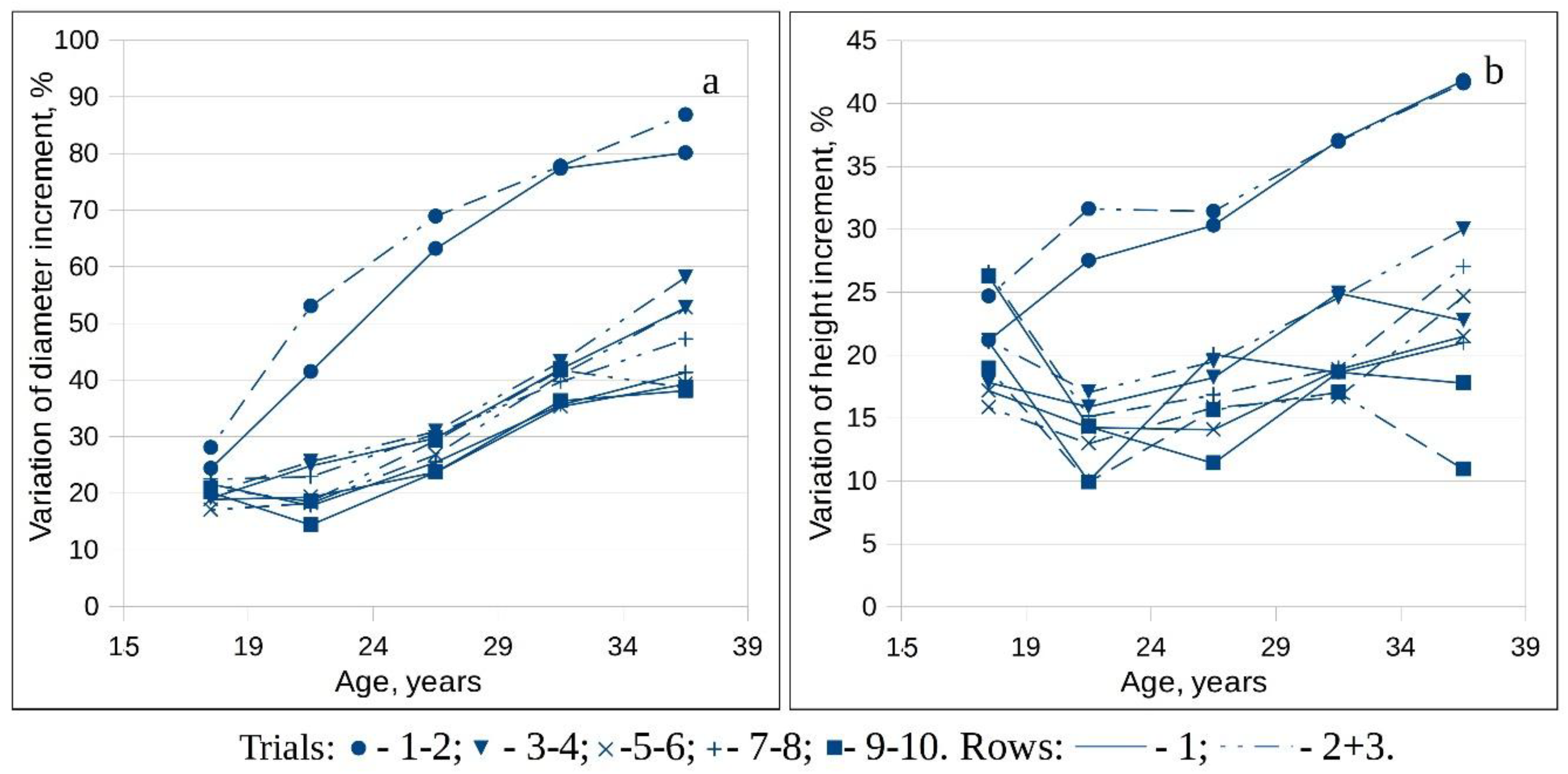
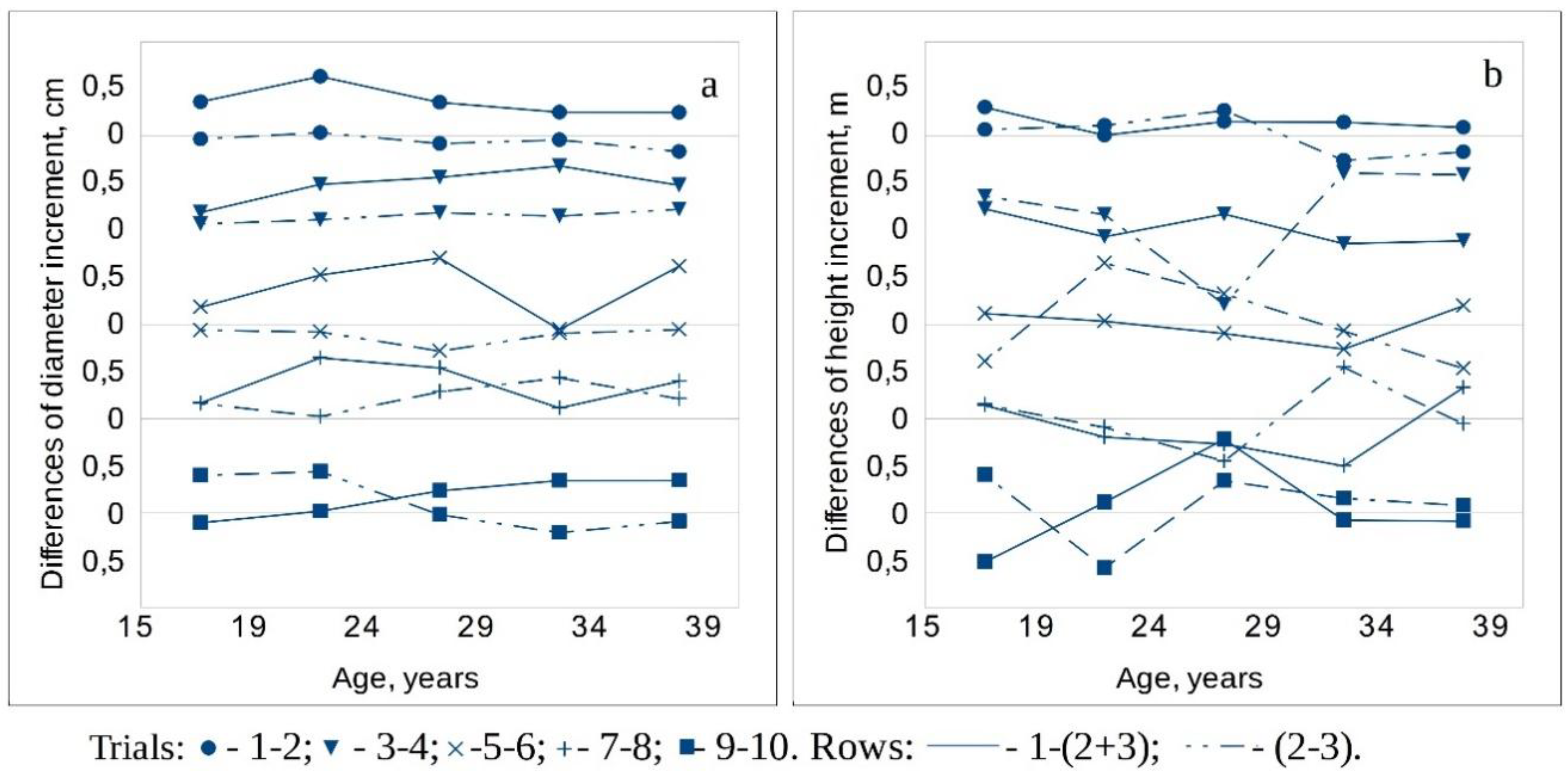
3.1. Analysis of Tree Diameter and Height Growth Differences Depending on Tree Row Position Relative to Strip Roads

The growth in diameter and height of the trees in each of the three groups of rows was estimated. For that purpose, diameter and height increments (

Table 2. Increment of trees growing in the bordering to strip road (1), in the second (2) and in the third (3) rows to strip road.

Number of Trial	Rows	Years of Measurements/Age of Stands
		92–95	95–00	00–05	05–10	10–15	92–95	95–00	00–05	05–10	10–15
		15–19	19–24	24–29	29–34	34–39	15–19	19–24	24–29	29–34	34–39
		Diameter Increment, cm					Height Increment, m
1–2	1	3.12	2.56	1.84	1.34	1.43	2.42	2.67	3.18	2.29	1.95
	2	2.74	1.93	1.46	1.08	1.13	2.15	2.64	3.13	2.09	1.76
	3	2.77	1.90	1.54	1.12	1.29	2.08	2.52	2.86	2.35	1.93
3–4	1	3.37	3.95	3.94	2.91	2.77	2.47	3.59	3.08	2.63	2.65
	2	3.20	3.49	3.43	2.28	2.36	2.52	3.69	2.70	2.97	2.88
	3	3.13	3.38	3.24	2.12	2.13	2.16	3.52	3.48	2.36	2.29
5–6	1	4.05	4.96	4.63	3.32	2.98	2.66	3.72	3.05	3,09	2.07
	2	3.84	4.41	3.83	3.34	2.34	2.38	3.90	3.32	3.34	1.74
	3	3.90	4.48	4.11	3.43	2.39	2.76	3.25	3.00	3.41	2.20
7–8	1	4.14	5.21	4.17	2.94	2.84	2.24	3.95	2.76	2.70	2.56
	2	4.02	4.56	3.71	2.95	2.50	2.13	4.06	2.87	3.45	2.21
	3	3.85	4.54	3.42	2.51	2.29	1.97	4.14	3.32	2.90	2.26
9–10	1	5.18	6.74	4.87	2.88	3.38	2.27	3.89	3.89	2.66	3.17
	2	5.42	6.87	4.63	2.46	3.00	2.93	3.66	3.20	2.73	3.28
	3	5.02	6.43	4.64	2.67	3.08	2.52	4.24	2.86	2.57	3.19

), their standard deviations, the difference between the increments of trees growing in second and third rows, as well as the difference between trees growing in first rows and those in second and third rows combined and the statistical significance of these differences (

Table 3. Statistical significance of growth difference between trees, growing in different rows.

Number of Trial	Combination of Rows	Years of Measurement/Age of Stands
		92–95	95–00	00–05	05–10	10–15	92–95	95–00	00–05	05–10	10–15
		15–19	19–24	24–29	29–34	34–39	15–19	19–24	24–29	29–34	34–39
		Diameter Increment					Height Increment
		Statistics t
1–2	2 − 3	−0.44	0.39	−0.70	−0.38	−1.19	1.42	1.41	2.62	−2.74	−1.58
	1 − (2 + 3)	7.26	9.09	4.47	3.46	2.80	9.08	0.20	2.22	2.34	1.42
3–4	2 − 3	0.95	0.83	0.93	0.85	0.91	6.83	1.70	−7.32	4.67	3.50
	1 − (2 + 3)	3.92	5.22	4.01	4.68	2.51	6.57	−1.10	2.46	−1.59	−1.13
5–6	2–3	−0.63	−0.52	−1.16	−0.31	−0.16	−6.98	7.82	3.03	−0.52	−4.46
	1 − (2 + 3)	2.78	4.91	4.25	−0.24	3.14	2.95	0.63	−1.28	−2.83	2.72
7–8	2 − 3	0.99	0.14	1.18	2.00	0.83	1.49	−0.83	−4.43	4.65	−0.37
	1 − (2 + 3)	1.58	5.46	3.36	0.69	2.17	2.39	−3.10	−3.31	−5.71	3.68
9–10	2–3	1.48	1.54	−0.05	−0.74	−0.28	3.32	−5.60	3.18	1.39	1.09
	1 − (2 + 3)	−0.54	0.13	1.09	1.85	1.58	−5.36	1.42	9.67	−0.83	−0.97

) were estimated.

Diameter and height increments. Diameter increment increased with decreasing growing density. The ratio between the diameter increment of trees growing in the most intensely thinned trials (9 and 10) and the densest trials (control trials 1 and 2) was 2–3 (Table 2). Diameter increment was highest during years 15–19 in trials 1–2 and years 19–24 in all other trials. After reaching the maximum, diameter increment decreased. Diameter increment for trees growing in the first row closest to the road exceeded the increment of trees growing in the second and third rows in almost all trials (Table 2). The maximum height increment was attained at 19–24 years in all trials with thinning and 5 years later in the control trials without thinning. The difference between the height increment of trees growing in first rows and those in second or third rows was not as regular and stable as for the diameter increment (Table 2).

Diameter and height increment variation. Variation of diameter and height increment will be presented in relational, comparative units, as variation coefficients (Figure 3). Variation of diameter increment was two or more times higher than variation of height increment. Variation of diameter increment increased with increasing age of trees from the beginning of the experiment (stand age 15 years) for trials 1–2 (control) and trials 3–4 with light thinning, whereas for the other trials, it increased from 19–24 years age, while variation of height increment increased in a similar way only in control trials 1–2. Height increment variation in all thinned trials (3–10), which had lower competition between trees for growing space, decreased during years 15–24 and increased in years 24–39 at a similar intensity to the control trial (Figure 3b). In most cases, the variations of diameter and height increment decreased with increasing thinning intensity. The variation of diameter increment as well as the variation of height increment in control (not thinned) stands was up to 1.6–2.0 times that of the trials with thinning, sometimes even higher. A regular and stable difference in variation of increment was not observed between trees growing in outer rows (adjacent to strip roads) and those growing in inner rows (second and third rows from the strip road, Figure 3).

Estimation of growth difference between trees growing in different rows. The differences in diameter increment and height increment between trees growing in second and third rows and between those growing in first rows and second plus third rows (combined) were analysed (Figure 4, Table 3).

Differences in the 4–5-year diameter increment between trees growing in second and third rows were not regular and stable; they ranged from -0.28 to +0.29 (0.44) cm. In trials 1–2 and 5–6, negative differences prevailed, meaning that the diameter increment of trees growing in third rows exceeded that of trees growing in second rows. Trials 3–4 and 7–8 exhibited the opposite result, characterized by higher increments in second row trees compared with the third row (Figure 4). Overall, the differences in diameter increment between trees growing in second and third rows were not statistically significant at a probability of 0.95; the t-statistic ranges from −1.19 to +1.54 (Table 3).

The diameter increment of trees growing in the first row next to a strip road in most cases exceeded the diameter increment of trees growing in the second and third (inner) rows. The differences in increment for each 4–5 year period attained 0.56–0.75 cm. The differences are statistically significant for 17 cases out of 20, primarily in trials 1–8 (Table 3). Only in trials 9–10, with very intensive and early thinning, was the difference in diameter increment between trees in inner and outer rows statistically insignificant (t = −0.54 to +1.85). The trees in trials 9–10 had approximately the same growing space and conditions for growth across all of the rows due to very low density.

Differences in the 4–5-year increment in height between trees growing in second and third rows were especially irregular and random. Within the same trial (for example, trials 3–4) they ranged from −0.78 to + 0.61 m (Table 3). In all trials, almost equally positive and negative values of differences between the height increments of trees growing in the second and third rows were observed. In 10 cases of 25, the differences were not statistically significant, as the t-statistic did not exceed a value of 2.0. The high variation in height increment differences among the trees growing in second and third rows did not allow the differentiation of these groups based on the specific height growth of trees.

The differences in the height increment of trees between those growing in the first row next to a strip road and those growing in second and third rows was also characterized by very high variation (Table 3). Differences in periodic height increment ranged from −0.50 to + 0.79 m. Negative differences represented 11 cases out of 25. Statistically significant differences were found for 15 cases out of 25. The results of this analysis show that height growth is not a useful basis for differentiating trees according to their row position.

The results ascertained related to the random pattern of diameter and height growth differences between trees growing in second and third rows, allowed subsequent analyses to use two groups of rows: inner (second and third from the road) and outer (first row, bordering the strip road).

3.2. Analysis of Differences in the Main Parameters of Trees Growing in the First Row Next to a Strip Road Relative to All Other Rows

The mean parameters of trees—mean height, mean diameter, density, gross increment and growing stock volume on inner and outer rows were estimated (

Table 4. The mean characteristics (T) of trees growing on inner rows (2, 3) and ratio of characteristics (K_T) of trees growing on outer (1) and inner (2, 3) rows.

Number of Trial	Years of Measure-Ment	Age	Height		Diameter		Number of Trees		Gross Increment		Growing Stock Volume
			T, m	KT	T, cm	KT	T, pc/ha	KT	T, m3/ha	KT	T, m3/ha	KT
1–2	1992	15	4.0	1.00	4.3	1.02	5079	1.00	22	1.06	22	1.06
	1995	19	6.1	1.05	7.1	1.06	5079	1.00	53	1.21	75	1.17
	2000	24	9.2	1.01	9.4	1.10	4734	1.06	98	1.33	171	1.27
	2005	29	12.9	1.01	11.6	1.10	3728	1.18	131	1.45	283	1.40
	2010	34	15.5	1.01	13.2	1.10	3328	1.21	121	1.51	390	1.46
	2015	39	18.1	1.01	15.3	1.09	2757	1.30	136	1.60	500	1.54
3–4	1992	15	4.7	0.98	5.2	1.00	3573	1.08	22	1.08	22	1.08
	1995	19	6.9	1.01	8.3	1.02	3573	1.08	54	1.19	77	1.16
	2000	24	11.0	1.01	12.6	1.06	2068	1.11	103	1.26	151	1.23
	2005	29	14.3	1.01	16.7	1.08	1252	1.19	112	1.42	200	1.38
	2010	34	17.1	1.01	18.9	1.11	1152	1.17	100	1.51	281	1.43
	2015	39	20.0	1.00	21.2	1.13	1079	1.15	130	1.43	386	1.42
5–6	1992	15	4.3	1.00	4.9	1.04	2412	1.07	13	1.16	13	1.16
	1995	19	6.8	1.03	8.7	1.06	2412	1.07	44	1.20	56	1.19
	2000	24	11.0	1.00	14.1	1.05	1333	1.24	86	1.36	119	1.35
	2005	29	14.4	0.99	18.5	1.08	753	1.42	90	1.54	145	1.63
	2010	34	17.8	0.98	21.9	1.06	707	1.40	99	1.45	234	1.54
	2015	39	19.7	0.99	24.4	1.09	680	1.40	82	1.78	307	1.62
7–8	1992	15	4.0	1.10	4.8	1.08	1433	1.10	7	1.33	7	1.33
	1995	19	6.1	1.08	8.8	1.07	1424	1.10	24	1.32	31	1.33
	2000	24	10.3	1.03	13.4	1.09	1415	1.10	77	1.33	108	1.33
	2005	29	13.8	0.99	18.0	1.09	889	1.19	85	1.36	156	1.38
	2010	34	17.0	0.96	20.9	1.08	771	1.30	90	1.30	223	1.43
	2015	39	19.3	0.98	23.4	1.08	753	1.26	90	1.57	308	1.43
9–10	1992	15	4.7	1.00	5.9	1.00	671	1.25	5	1.28	5	1.28
	1995	19	7.5	0.93	11.2	1.00	671	1.25	22	1.12	27	1.16
	2000	24	11.3	0.96	17.9	1.00	662	1.27	68	1.22	95	1.21
	2005	29	14.3	1.03	22.4	1.01	617	1.30	86	1.46	169	1.37
	2010	34	17.1	1.02	25.1	1.02	590	1.31	78	1.43	240	1.39
	2015	39	20.4	1.01	28.2	1.03	580	1.31	118	1.43	353	1.41

).

Mean height. Mean height was estimated using modelled heights and Lorey’s formula. Heights for every tree were modelled using a general model [13] and the measured heights and diameters of sample trees, as well as the mean diameter of all trees with measured DBHs.

The intensity of height growth of spruce trees in the experiment increased with age. The site index for all trials during 24 years increased by 5–7 m (Table 1). This is a typical growth pattern, with increasing growth in the first two to three decades of the formation of a stand on a former agricultural site due to the roots of trees reaching the soil layer saturated by minerals during cultivation of crops.

The mean heights of trees growing in inner rows increased over 24 years by 14–15 m, i.e., an average of 0.6 m per year (Table 4). The mean heights of trees growing in outer rows of trials 1–4 were 1% taller, while in trials 5–8 after decreasing density up to 800–1200 trees/ha, the mean heights of trees in outer rows was 1%–2% less than in inner rows (Table 4). This indicates that the mean height differences of trees growing in inner and outer rows may have a minimal influence on differences in productivity.

Mean diameter. Site index D₁₀₀, characterizing the tree diameter growth conditions, did not vary as much with age as with the growing density conditions of the different trials. The diameter growth conditions in the control (1–2) trial were fairly stable (on average 34 cm) across the entire duration of the experiment. The diameter growth site index D₁₀₀ in all other trials increased to 52–53 or even 60 cm when the tree density became 800–600 trees/ha (Table 1). Compared with the height growth of trees, the diameter growth is more sensitive to the density of trees in the stand (Table 4). This was especially apparent in the control trial, where the additional growing space provided by the road is very productively used by the trees growing on rows neighbouring roads. The mean diameter of trees growing in outer rows in trials 1–4 exceeded the mean diameter of trees in inner rows by up to 1.09–1.13 times, while for all other trials excluding trials 9–10, the differences did not exceed 1.08–1.09. The differences in the mean diameters of trees in outer rows compared with the mean diameter of trees in inner rows increased with age for all trials (Table 4). Such differences in mean diameter will result in corresponding and essential differences in basal area and stem volume of 16%–26%.

Number of trees. Number of trees, specific for every trial, was achieved by seeking an equidistant distribution of trees per trial. This condition automatically leads to a higher density of trees in outer rows. The number of trees in the outer rows of all trials exceeded the number of trees in inner rows by 1.06–1.40 times (Table 4). Differences in the number of trees between outer and inner rows increased with age and with decreasing stand density. Such differences are characteristic not only in trials with artificially regulated density, but also in trials with natural self-thinning. The natural formation of higher density in rows neighbouring roads confirms the objectivity of the artificial formation of higher density in outer rows.

Gross increment. The gross periodical increment (GPI) of trees growing in inner rows increased with age, approaching a maximum at the age of 39 years. The GPI values of trees growing in inner rows in trials 1–4 were very similar. The GPI values of trees in the other trials at 29–39 years of age were 65%–75% of the GPI of trials 1–4 (Table 4). The ratio of the GPI of trees growing in rows bordering the road to that of inner rows increased with age more intensively with increasing diameter and number of trees (Table 4). This means that the additional growing space created by the establishment of a road is very efficient for increasing intensity of growth for all trials. The GPI of trees growing in outer rows exceeds the GPI in inner rows nine years after establishing the experiment by 22%–36%, while at twenty fourth years, that value is 43%–78%. The growth response to the additional growing space is comparatively high in all trials, including the control (1–2) trial and the trial with the lowest density of trees (9–10).

Growing stock volume. The estimated differences in mean diameters, mean heights and number of trees allow estimation of the differences in an integral characteristic: growing stock volume (Table 4). The trees of inner rows in the control trials, 1–2, attained the largest growing stock volume at all observed ages. In all other trials, the attained growing stock volume reached 62%–77% of the growing stock volume of trials 1–2. The ratios of growing stock volume of trees in outer rows and in inner rows increase in a very similar way to the ratios of GPI. Ratios of growing stock volume of trees in outer and inner rows for all trials and for all ages ranged from 0.03–0.07 less than ratios for GPI, as the result of the trees removed by felling or by self-thinning.

3.3. Analysis of Growth Losses and Capability to Compensate for Them Due to Different Structure and Growth of Trees in the First Row Next to a Strip Road

More intensive growth of trees on rows, directly neighbouring a strip road, is able to compensate for the main losses due to use of productive area for a strip road. The level of growth compensation in our case was estimated by Formulas (1–3). At the beginning of the experiment, at 15 years of age in all trials, a compensation for GPI losses of 12%–67% was observed (Figure 5a). The least compensation was observed in the control (1–2) trial. Compensation of GPI losses in this trial increased very intensively with age; a similar pattern was observed for trials 5–6.

Complete, 100% compensation for growth losses occurred at 28 years of age in trials 5–6 (Figure 5a), and in trials 1–2 five years later. In all other trials, compensation for growth losses had attained or was approaching 100% at age 34–39 years. This only varied in trials 9–10, with the lowest density of trees, in which compensation for GPI losses in the last decade only reached 86%–91% and was very stable during the last 10 years.

Very similar tendencies were observed for the investigation of growing stock volume compensation. Compensation for growing stock volume in trials 3–4, 7–8 and 9–10 stabilized at the 73%–85% level in the last decade. In trials 5–6 and 1–2, the compensation level reached 100% at ages 27 and 37 years, respectively.

4. Discussion

Rational design of strip roads requires answering two questions: (1) what is the response of trees growing at the edge of strip roads, and (2) what total losses or gains result from establishing strip roads in stands?

The first question is closely related to growth patterns in various structural elements of stands. The growth of trees bordering open areas, gaps, and linear objects depends on the type of open area and the state and specific growth of the trees [5,15,16,17]. Open areas formed due to death of weak trees grown in excessively dense conditions, can be prescribed to the areas close to which growing trees cannot compensate for the gross increment losses due to decreased productive area within the open area [5]. The growth pattern of trees growing in the edge zone of the stand changes with age [6]. Trees in the edge zone during stand formation experience conditions of lower density and attain greater mean diameter, lower mean height and less productivity. Later, in maturity, trees in the edge zone maintain higher growth intensity and attain higher productivity—up to 15%–20% more compared with the interior zone of the stand.

Researchers [4,18,19,20,21,22] investigating the influence of strip roads on stand productivity have indicated that trees growing no farther than 2–3 m from strip roads exhibit increased diameter growth. Almost all previous researchers have found that that the strongest responses are exhibited by the trees at the edge of the strip road, with an increasing intensity of growth with increasing of time after thinning. The diameter increment of spruce trees in the edge zone 1.5–1.57 m from the strip road increases by 20%–55% compared with the growth of trees in the central zone, 9–16 m from the strip road, whereas in the zone 1.5–3.1 m from the road, the increase is three times less [18]. Isomaki [23] even found that the increment of the trees located behind the edge trees decreased slightly due to increased shading by the edge trees, but such an effect was not confirmed by Makinen et al. [20]. Different widths of strip road (5.6 and 6.8 m.) do not change the intensity of diameter growth of trees at the edge of the strip road [7]. Investigations made in this field allow us to conclude that increased growing space, resulting in increased diameter growth is among the main factors that compensate for growth losses due to establishment of strip roads. Other researchers [20,21] have also indicated that additional nutrients from felling residuals, concentrated on the strip roads, are another main factor influencing additional increase in diameter growth.

Together with the positive influence of strip roads on tree growth, other researchers [24] also ascertained that 32 years after roads were used for logging, soil remained heavily compacted, resulting in growth reduction within the road and transition zones, resulting in growing stock losses of 11.8% for the total area. A negative influence of strip roads on the growth of trees can also occur in cases where very heavy equipment is used or uncareful harvesting is applied and trees bordering strip roads are damaged [21,25,26,27,28].

In our research project, strip roads were established together with the establishment of the stand, leaving every sixth row treeless. Manual techniques were used for thinning, and felling residues were spread across all areas or removed from the area. Light equipment was used for transportation of wood, and no damages in the trial area were allowed. Therefore, the main factor causing additional growth in our case is increased growing space for trees bordering the strip roads. The results of our study, based on regular measurements of permanent plots over 24 years, supplement the existing knowledge about the growth of trees close to open areas on the edges of stands and illustrate that the growth of trees in the outer row of spruce plantations exceeds the growth of trees in inner rows (second and third rows from the road) from the beginning of the experiment, at a stand age of 15 years. No significant difference between the diameter growth of trees growing in the second and third rows from the strip road was observed. Analogous results have also been observed in pine stands [22].

The increased total yield of outer trees is a result of not only increased diameter growth, but also a higher density of trees in the edge row. The main precondition to achieve maximum growth for every tree in every trial with different density regimes was to guarantee more or less equal growing space for every tree. Trees growing at the edge of a strip road have the chance to use that additional space. That additional space allows for a higher density of trees along the edge row compared to the inner rows. The higher density of trees in rows bordering the strip roads in the naturally developing forest stands in the control trials confirmed the correctness of the practice of leaving a higher density in rows bordering the strip roads during thinning.

In the same way, we confirmed the results of others researchers [7] that differences in trees height growth between outer and inner rows are insignificant, and that tree heights in forest and stand edges are lower than in inner zones [3,29].

The growth of trees in outer rows increases with age, and in 39 years the total GPI of outer trees exceeded the total GPI of trees growing on inner rows by 43%–78%.

The influence of strip roads on the productivity of plantations will, in general, depend on the width of the strip road as well as the width of the spacing between roads. In a case where the road width of 3.5 m is increased to 5.25 or 7.0 m, the capability of trees bordering the road to compensate for growth losses will decrease correspondingly by 50% or 33.3% (Formula (4, 5)). Assuming that the additional intensity of growth of trees bordering the strip road will remain approximately the same [20] whether one or two rows of trees is used for the establishment of strip roads [7,18], the compensation level of productivity losses will decrease with increasing width of the strip road and decreasing spacing between roads (Formula (6),

Table 5. Estimation of productivity losses depending on width of strip road and width of strip of trees.

Width of Road		Width of Strip of Trees, m/Number of Rows, nT
		7/5			15.75/10			24.5/15
		KT
in m	Number of Rows, nR	1.25	1.5	1.75	1.25	1.5	1.75	1.25	1.5	1.75
		Losses, %
3.50	1	8.3	0.0	+8.3	4.5	0.0	+4.5	3.1	0.0	+3.1
5.25	2	21.4	14.3	7.1	12.5	8.3	4.2	8.8	5.9	2.9
7.00	3	31.2	25.0	18.8	19.2	15.4	11.5	13.9	11.1	8.3

). The results of our investigation, expanded to a spruce plantation with an outside width of strip roads from 3.5 to 7.0 m and with a spacing between roads of 7.0 to 24.5 m (Table 5), showed a wide range of productivity losses. The expected productivity losses due to the establishment of strip roads for a typical situation—outside width of strip road 5 m, spacing between roads 16–24 m, and ratio of productivity of trees bordering the strip road to productivity of trees inside stand 1.5—will be approximately 6%–8%. Investigations of 40–67-year-old spruce stands in southern Finland [12], showed very similar results, summarizing that strip roads with a 5.1 m outside width, allocated every 30 m and occupying 17% of the stand area, decreased productivity by only 8%. A similar effect, of the growth of spruce trees neighbouring the strip road influencing a decrease of growth losses, has been ascertained by experimental trials in the Czech Republic [7] and in Sweden [18] as well as by using a simulation method [4].

The results obtained in the presented research allow stand managers to optimize the width and spacing of strip roads on spruce plantations depending on the equipment used for silviculture measures, which is especially important for intensive forest growing in spruce plantations with shortened rotation times [1,2].

5. Conclusions

• The growth in the height and diameter of trees in the second and third (inner) rows from a road is statistically homogenous, but this growth is statistically different (at probability 0.95) from the growth of trees in the first (outer) row along a road, depending on age and thinning regime.
• Trees growing in outer rows are distinguished by larger mean diameter, higher density, in some cases by higher height and always by higher growing stock and gross annual increment compared with trees growing in inner rows:

  -

  The diameter of trees in outer rows exceeds diameter of trees in inner rows by up to 9%–13%;

  -

  Differences in the mean height of trees between outer and inner rows may reach ±2%–4%, but these differences are not statistically significant;

  -

  The number of trees in outer rows exceeds the number of trees in inner rows by up to 30%–42%, with differences increasing with increasing stand age;

  -

  The gross increment of trees in outer rows at age 29–39 years exceeds the increment of inner rows by up to 60%–78%;

  -

  The growing stock volume accumulated in outer rows exceeds that accumulated in inner rows by up to 42%–63%.

• Differences in mean diameter and the number and growing stock volume of trees in outer versus inner rows increase with increasing age and decrease with increasing intensity of thinning.
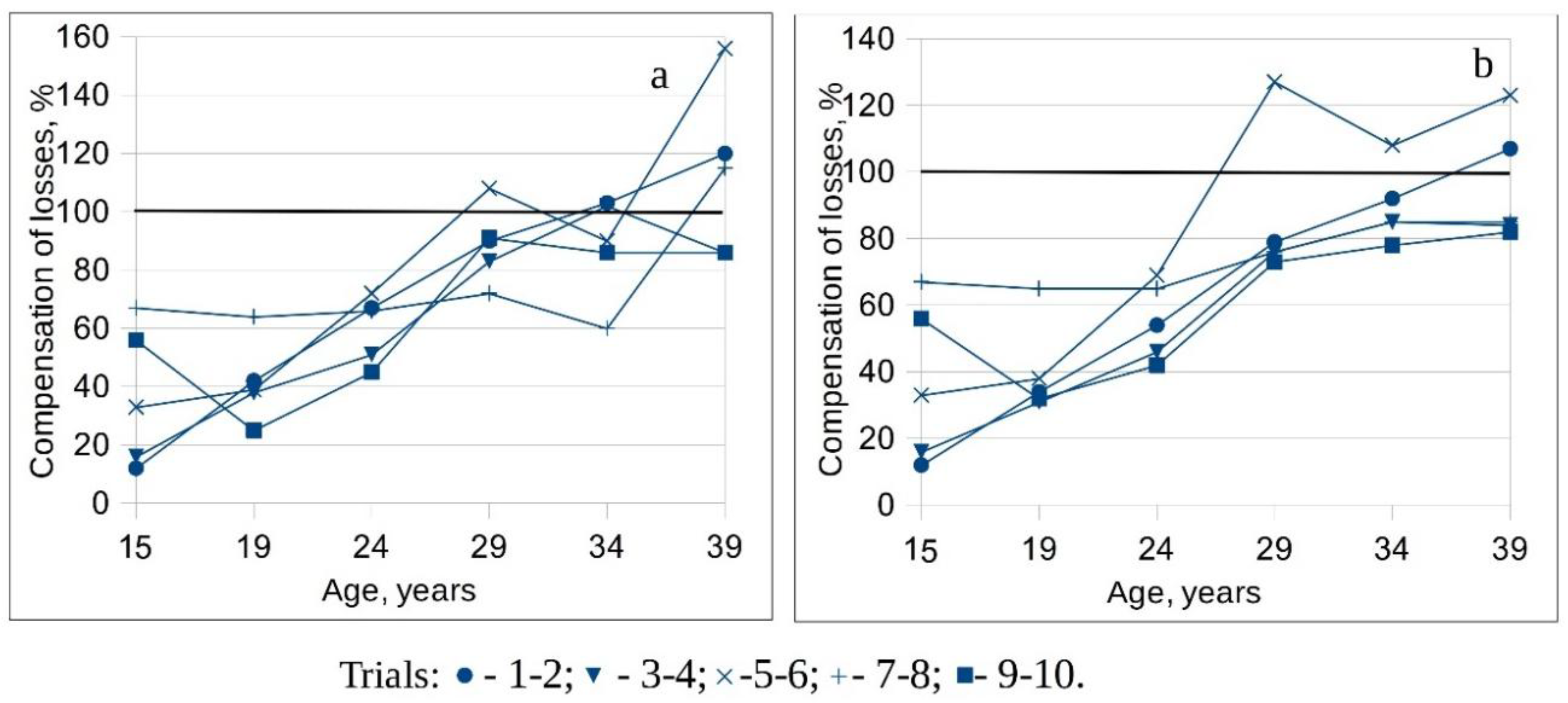
• More intensive growth and density of trees in outer rows may compensate for losses of GAI due to the establishment of a road 3.5 m in width by 12%–67% at 15 years and by 86%–156% at 39 years.
• Complete compensation for GAI losses occurs in the control trial at 33 years of age, in the 4-time thinning trial (5–6) at 28–34 years age, and in the 2-time thinning trial (7–8) at 38 years of age. Compensation of GAI losses for 1-time thinning (trial 9–10) reached 86%–91% and stabilized at 29–39 years of age.
• The influence of strip roads on the productivity of a plantation generally depends on the ratio of gross annual increment of trees in outer versus inner rows as well as the ratio of road width to the width of the spacing between roads. Productivity losses due to decreased productive area in spruce plantations with treed strips between roads approximately 20 m wide and 5 m wide roads are expected to be in the range of 6%–12%.

References

1. Shutov, I.V.; Maslakov, E.L.; Markova, I.A.; Polianskij, E.V.; Belkov, V.P; Gladkov, E.G.; Golovchanskij, I.N.; Riabinin, B.N; Morozov, V.A.; Shimanskij, P.S. Forest Plantations. Short Rotation of Spruce and Pine Stands; Lesnaja Promyshlennost: Моscow, Russia, 1984; p. 248. (In Russian) [Google Scholar]
2. Malinauskas, A. Miško Želdinių Pradinis Tankumas (Initial Density of Forest Plantations); Lututė: Kaunas, Lithuania, 2008; p. 229. ISBN 978-9955-37-039-0. (In Lithuanian) [Google Scholar]
3. Kenstavičius, J.; Jakubonis, S.; Ožeraitis, V. Gretimo medyno įtaka želdiniams (Influence of the adjacent stand to plantations). Girios 1984, 5, 8–10. (in Lithuanian). [Google Scholar]
4. Niemisto, P. A simulation method for estimating growth losses caused by strip roads. Scand. J. For. Res. 1989, 4, 203–214. [Google Scholar] [CrossRef]
5. Saladis, J. The relationships between the gap structure, stand age, productivity, spatial distribution and competition of trees in pure Scots pine stands. Balt. For. 1999, 5, 11–18. [Google Scholar]
6. Kuliešis, A.A.; Kuliešis, A. Edge effect on forest stand growth and development. Balt. For. 2006, 12, 158–169. [Google Scholar]
7. Horak, J.; Novak, J. Effect of stand segmentation on growth and development of Norway spruce stands. J. For. Sci. 2009, 55, 323–329. [Google Scholar] [CrossRef] [Green Version]
8. Kuliešis, A.; Saladis, J. The effect of early thinning on the growth of pine and spruce stands. Balt. For. 1998, 4, 8–16. [Google Scholar]
9. Kuliešis, A.; Saladis, J.; Kuliešis, A.A. Development and productivity of young Scots pine stands by regulating density. Balt. For. 2010, 16, 235–246. [Google Scholar]
10. Buivydaitė, V.V.; Vaičys, M.; Juodis, J.; Motuzas, A. Lietuvos Dirvožemių Klasifikacija (Classification of the Soils of Lithuania); Lietuvos Mokslas: Vilnius, Lithuania, 2001; p. 139. ISBN 9986-795-11-8. (In Lithuanian) [Google Scholar]
11. Vaičys, M.; Beniušis, R.; Karazija, S.; Kuliešis, A.; Raguotis, A.; Rutkauskas, A. Miško Augaviečių Tipai (Forest Site Types); Lututė: Kaunas, Lithuania, 2006; p. 95. ISBN 9955692413. [Google Scholar]
12. Isomaki, A.; Niemisto, P. Effect of strip roads on growth and yield of young spruce stands in Southern Finland. Folia For. 1990, 756, 36, (In Finnish with English Summary). [Google Scholar]
13. Kuliešis, A. Lietuvos medynų prieaugio ir jo panaudojimo normatyvai. In Forest Yield Models and Tables in Lithuania; Girios Aidas: Kaunas, Lithuania, 1993; p. 384, (In English and Lithuanian). [Google Scholar]
14. Kuliešis, A.; Kasperavičius, A.; Kulbokas, G.; Kvalkauskienė, M. Lietuvos Nacionalinė Miškų Inventorizacija 1998–2002. Atrankos Schema, Metodai, Rezultatai. Lithuanian National Forest Inventory 1998–2002; Sampling Design, Methods, Results; Naujasis Lankas: Kaunas, Lithuania, 2003; p. 254. ISBN 9988-03-185-9. (In English and Lithuanian). [Google Scholar]
15. Kairiukshtis, L.; Ozolincius, R. Dynamic of growth and structure of crown in the process of biotic community formation. Lesnoe hoziajstvo 1985, 5, 47–50. (In Russian) [Google Scholar]
16. Oliver, C.D.; Larson, B.C. Forest Stand Dynamics, Updated Edition; John Wiley & Sons Inc.: Hoboken, NJ, USA, 1999; p. 521. ISBN 13:978-0471138334. [Google Scholar]
17. Bowering, M.; LeMay, V.; Marshal, P. Effects of forest roads on the growth of adjacent lodgepole pine trees. Can. J. For. Res. 2006, 36, 919–929. [Google Scholar] [CrossRef]
18. Eriksson, H. New results from plot no. 5 at Sperlingsholm estate in southwestern Sweden in the European Stem number Experiment in Picea abies. Scand. J. For. Res. 1987, 2, 85–98. [Google Scholar] [CrossRef]
19. Eriksson, H.; Johansson, U.; Karlsson, K. Effects of Extraction Roads Width and Thinning Pattern on Stand Development in an Experiment with Norway Spruce (Picea abies (L.) Karst; Report No 38; Swedish University of Agricultural Sciences, Department of Forest Yield Research: Uppsala, Sweden, 1994; p. 23, (In Swedish, Summary in English). [Google Scholar]
20. Makinen, H.; Isomaki, A.; Hongisto, T. Effect of half-systematic and systematic thinning on the increment of Scots pine and Norway spruce in Finland. Forestry 2006, 79, 103–121. [Google Scholar] [CrossRef]
21. Wallentin, C.; Nilsson, U. Initial effect of thinning on stand gross stem-volume production in a 33-year-old Norway spruce (Picea abies (L.) Karst.) stand in Southern Sweden. Scand. J. For. Res. 2011, 26 (Suppl. 11), 21–35. [Google Scholar] [CrossRef]
22. Stempski, W.; Jablonski, K. Differentiation of tree diameters at strip roads in a young pine tree stand. Acta Sci. Pol. 2014, 13, 37–46. [Google Scholar]
23. Isomaki, A. Effects of line corridors on the development of edge trees. Folia For. 1986, 678, 30, (In Finnish with English Summary). [Google Scholar]
24. Wert, S.; Thomas, B.R. Effects of skid roads on diameter, height, and volume growth in Douglas-fir. Soil Sci. Soc. Am. J. 1981, 45, 629–632. [Google Scholar] [CrossRef]
25. Isomaki, A.; Kalio, T. Consequences of injury caused by timber harvesting machines on the growth and decay of spruce (Picea abies L. (Karst.). Acta For. Fenn. 1974, 136, 1–25. [Google Scholar] [CrossRef]
26. Wasterlund, I. Growth reduction of trees near strip roads resulting from soil compaction and damaged roots. A literature survey. Sver. Skogsvardsforb. Tidskr. 1983, 81, 97–109, (In Swedish with English Summary). [Google Scholar]
27. Andersson, L. Influence of stem wounds on the growth of Scots pine. In Proceedings of the meeting of IUFRO Project Group P4.02 and Subject Group S1.05-05, Scandinavia (Sweden, Norway, Denmark), 9–18 June 1987; Knutell, H., Ed.; Swedish University of Agricultural Sciences: Garpenberg, Sweden, 1987; pp. 53–63. [Google Scholar]
28. Nadezhdina, N.; Čermak, J.; Neruda, J.; Prax, A.; Ulrich, R.; Nadezhdin, V. Roots under the load of heavy machinery in spruce trees. Eur. J. For. Res. 2006, 125, 111–128. [Google Scholar] [CrossRef]
29. Deltuva, L.; Marozas, V. Pamiškės efektas eglynų sudėčiai ir struktūrai (Influence of edge effects on spruce forest composition and structure). Miskininkyste 2000, 1–2, 5–11. (In Lithuanian) [Google Scholar]
Figure 1. Dynamics of the main gradients of climate—temperature (a) and precipitation (b) according to data of meteorological station “Vėžaičiai” located 7 km from the trial location.
Forests 09 00640 g001
Figure 2. The scheme of experimental area design.
Forests 09 00640 g002
Figure 3. Changes of diameter (a) and height (b) increment variation based on age, density of growth (trials) and position of tree rows in relation to strip road.
Forests 09 00640 g003
Figure 4. Changes of diameter (a) and height (b) periodical (4–5 years) increment differences between trees, growing in the 1 and 2 + 3 rows as well as between 2 and 3 rows depending on age and density of growing (trials).
Forests 09 00640 g004
Figure 5. Changes of level compensation of gross increment (a) and accumulated in stand growing stock volume losses (b) due to more intensive growth of trees in rows neighboring to strip road of 3.5 m width depending on age and growing density (trials).
Forests 09 00640 g005