Nearest Neighborhood Characteristics of a Tropical Mixed Broadleaved Forest Stand

Abstract

Structural complexity and local biodiversity of species-rich tropical forests can be characterized by their spatial patterns, which contribute to species intra- and interspecific interactions. Aiming to describe spatial patterns of species at fine spatial scales, we applied the quantitative analyses based on the relationships of nearest neighbors of conspecific and heterospecific trees. In a two-hectare plot of a tropical broadleaved forest stand in central Vietnam with minimal human influence, all tree individuals with diameter at breast height ≥ 2.5 cm were mapped and their characteristics were recorded. We applied two different types of analyses: (1) Intraspecific structural characteristics using nearest neighbor statistics; (2) overall interspecific associations through a classification scheme based on bivariate nearest neighbor distribution function D₁₂(r) and Ripley’s K function K₁₂(r). The findings showed that: (1) Most of studied species in the forest were highly mixed with other species, while conspecifics were regular to aggregated distribution at small spatial scales. Tree individuals with different diameter values were surrounded by heterospecific trees; (2) The majority of 306 species-species pairs showed spatial independence (66.7%), whereas 29.8% of all species showed an overall positive association and negative association consisted only a small percentage (3.5%) up to spatial scales of 50 m. We found significant evidences of the main ecological theories such as dispersal limitation, Neutral theory, Janzen-Connell hypothesis, and other effects like the stochastic dilution. We suggest using both the bivariate distribution of the structural parameters and the spatial point pattern analysis based on nearest neighbor distance as advantageous approaches for further understanding of population structure, as well as discovering and protecting biodiversity in the future.

1. Introduction

A central aim in ecological study is to understand processes and mechanisms controlling the distribution and abundance of species [1]. Understanding various ecological mechanisms and processes that influence species assemblage are critical to get deep insights on species associations and community structure. Analyzing the spatial patterns of species are therefore of main interest in community ecology to figure out the underlying mechanisms and to test different ecological theories [2,3,4]. Several processes—such as competition or facilitation, dispersal limitation, habitat preference, Janzen-Connell hypothesis—that have been proposed for explaining community structure and species coexistence in species-rich forests are mainly based on spatial characteristics of species associations [5].

For examples, the intraspecific aggregation could be described by dispersal limitation or ecological niches and lead to reduce the importance of interspecific competition [6,7]. Inversely, the spatial segregation also involves competitive interaction of competitively superior species which prevent the elimination of inferior species, therefore promoting species diversity [8,9]. Janzen-Connell hypothesis, for instance, was proposed to describe species coexistence in ecosystems such as tropical forests. This hypothesis suggests that in forest communities with high richness, tree individuals tend to be regularly distributed according to their conspecifics, probable parent trees [10], and even trees closely related to them [11,12,13,14]. Therefore, the theory predicts more negative interactions of conspecifics and more positive interactions of heterospecifics than expected by chance. Species coexistence in diverse communities such as tropical forests can also be described by neutral theory, which assumes that species associations are assembled by dispersal limitation and demographic stochastics [15]. Similarly, previous studies suggested that stochastic dilution effect that assumes independent placement of individuals of different species can well explain species coexistence in tropical forests [3,16,17]. The stochastic dilution effect assumes hypotheses of intraspecific clustering, independence of interspecific interaction and abundance of species following a hollow curve distribution [18].

A number of methods for describing forest structural attributes have been largely developed for decades. However, an exact description of small-scale structural attributes is considered to be increasingly importance [19]. During these last decades, well-known estimations based on relative tree positions are the Clark and Evans aggregation index [20], segregation index of Pielou [21], Diggle’s F and G functions [22], and Ripley’s K function [23]. These functions use tree-tree distances to calculate the cumulative or noncumulative distribution of tree individuals in a range of spatial scales. Recently, new individual tree indices, such as uniform angle index, species mingling and dominance [24,25,26], have been developed. The basic idea of these indices is to characterize the neighborhood of a reference tree by using its n-nearest neighbors. The techniques of nearest neighbor statistics allow us determining the relationship within neighborhood groups of trees such as species and size class at small scales. Greater inhomogeneity in species and homogeneity in size classes indicate greater structural diversity [27].

In this study, our overall goal is to characterize spatial attributes of neighborhood trees by applying the current techniques of nearest neighbor statistics. Therefore, we used three structural indices [27], Ripley’s K function K₁₂(r) and nearest neighbor distribution function D₁₂(r) [3]. For a better understanding of structural units, we used bivariate distribution in which combines pairs of two structural units for each species, such as mingling-uniform angle index, mingling-dominance and dominance-uniform angle index. To clarify species-species association, we quantified how the trees of given species 2 were distributed within local neighborhoods of trees of a focal species 1. We hypothesized that the mechanism of Janzen-Connell can cause positive associations of heterospecifics and negative interactions of conspecifics. Moreover, if stochastic dilution effect governs species associations, the proportion of species pairs with no association is significantly high. We performed two different types of analyses. Firstly, we investigate species-based interactions of conspecifics and heterospecifics using the indices based on distance to nearest neighbor (Analysis 1). Secondly, we analyze overall species associations of heterospecifics through a classification scheme defined by bivariate Ripley’s K function K_ij(r) and cumulative nearest neighbor distribution function D_ij(r) (Analysis 2).

2. Materials and Methods

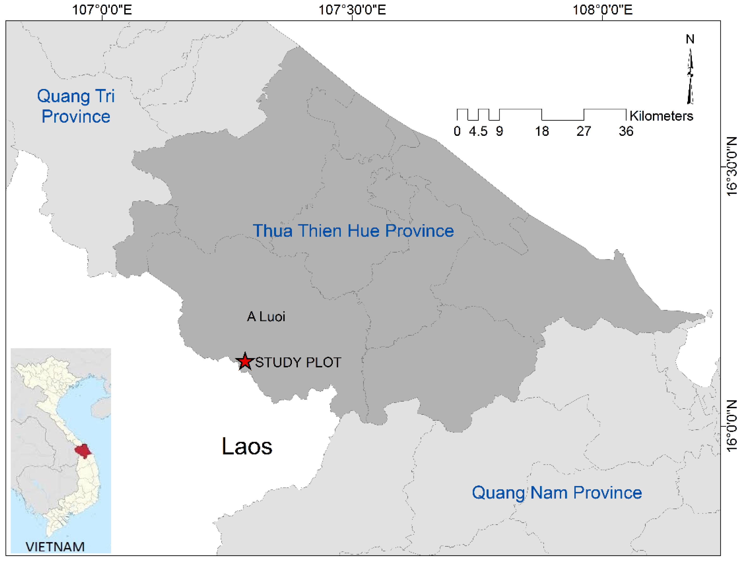
2.1. Study Site and Data Collection

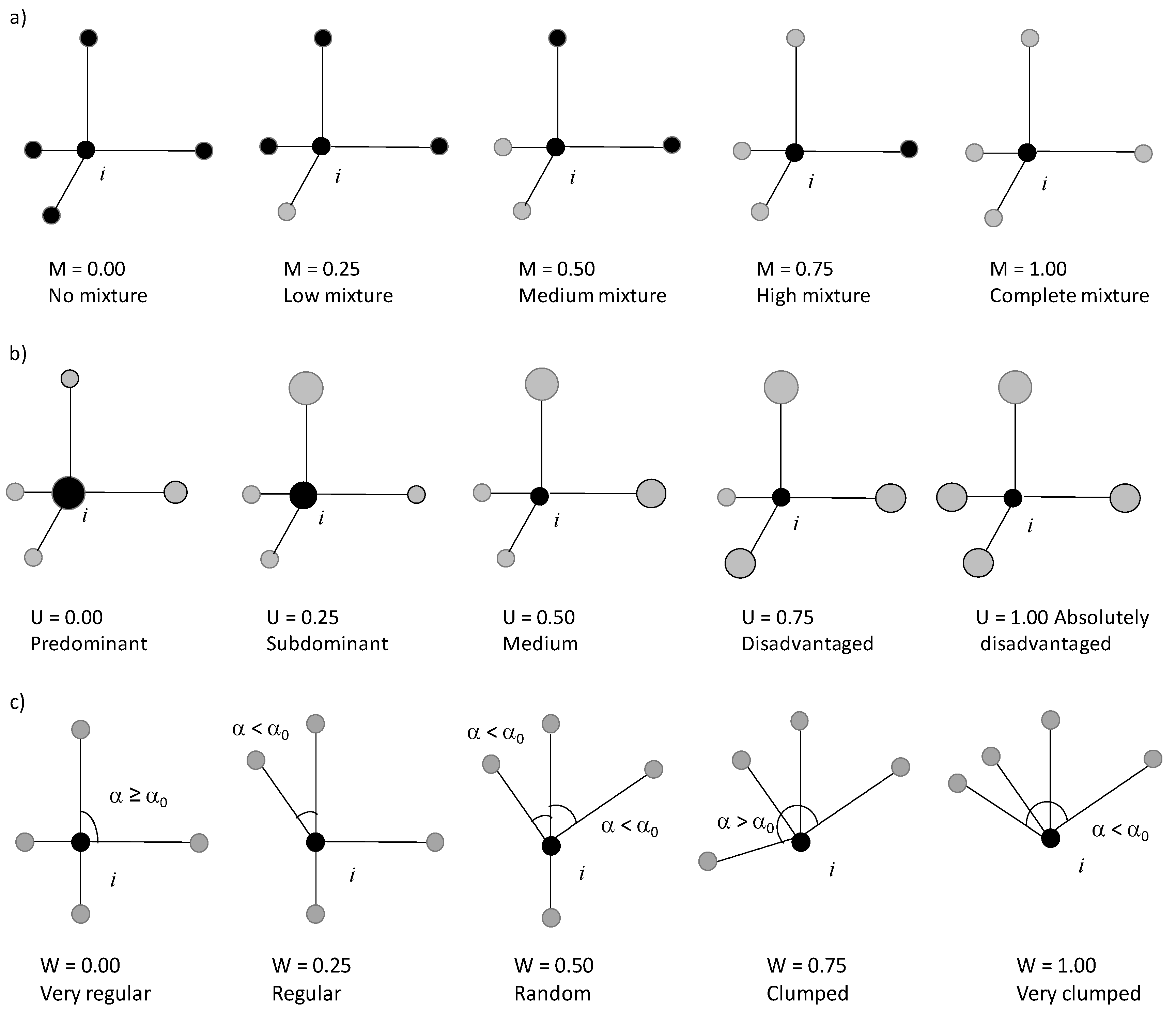
A 2-ha plot was designed at a location of 16°08.35′ N and 107°16.68′ E on a tropical broadleaved forest stand in Aluoi district, Thuathien-Hue province, North-Central Vietnam (Figure 1). Here, the climate is tropical monsoon with the average annual temperature of 25 °C and precipitation of 3500 mm. The rainy season lasts from September to December owning 70–80% of the total precipitation. Soils are mainly light yellow to dark yellow ferralic acrisols. A grid of 200 subplots (10 m × 10 m) was then created in which all trees with diameter at breast height (DBH) ≥ 2.5 cm was mapped. A tree is considered as two trees if branched below DBH is required as methodology in forest inventory [28]. Tree position (x, y coordinates) was recorded by using a laser distance measurer (Leica Disto D5) and compass; other characteristics such as species and DBH were also investigated. Elevation of the plot ranges from 625 to 660 m a.s.l, with an average slope of 25 degrees. No visible human influence could be detected in this mature secondary tropical forest (e.g., the human signs are no longer evident).

2.2. Data Analysis

In this study, we applied current techniques of nearest neighbor statistics which are based on the assumption that the spatial structure of a forest stand is determined by the distribution of specific structural relationships within neighborhood groups of trees. A forest stand is composed by neighborhood structural units of n-trees. We used three structural indices proposed by von Gadow and Hui [29] such as species mingling, dominance and uniform angle index to describe homogeneity or heterogeneity of trees through a variety of species, diameter classes and spatial arrangements with Equations (1)–(3) [24,25,26,30].

Moreover, we used two summary statistics applicable to completely mapped bivariate point patterns such as the K function K₁₂(r) and the cumulative nearest neighbor distribution function D₁₂(r) in order to categorize the possibly heterogeneous species-species associations. This allowed us to quantify how the individuals of species 2 are distributed within local neighborhoods of the individuals of a focal species 1. Therefore irrespective sho––wing tree-tree distance is regulated by external effects of the environment, by internal effects of species interactions or by intraspecific clustering [3].

2.2.1. Analysis 1—Intraspecific Patterns

Species mingling (M): describes the species composition and spatial pattern of forest trees. It is defined as the proportion of the n-nearest neighbours that are different species from the reference tree (Figure 2a).

$${\mathrm{M}}_{\mathrm{i}}=\frac{1}{4}{\displaystyle \sum }_{j=1}^4{v}_j$$

(1)

v_j = 1 if neighbor j is not the same species as reference tree i, otherwise v_j = 0.

Dominance (U): describes the size differentiation between a reference tree and its four nearest neighbors. It is defined as the proportion of n-nearest neighbors that are smaller than reference tree (Figure 2b).

$${\mathrm{U}}_i=\frac{1}{4}{\displaystyle \sum }_{j=1}^4{v}_j$$

(2)

v_j = 0 if neighbor j is smaller than reference tree i, otherwise v_j = 1.

Uniform angle index (W): describes the degree of regularity for the four nearest neighbors as reference tree. It is defined as the proportion of angle (α) smaller than the standard angle α₀ (Figure 2c).

$${\mathrm{W}}_i=\frac{1}{4}{\displaystyle \sum }_{j=1}^4{w}_j$$

(3)

W_i = 1 if α_j < α₀, otherwise W_i = 0, α₀ = 360°/(n + 1).

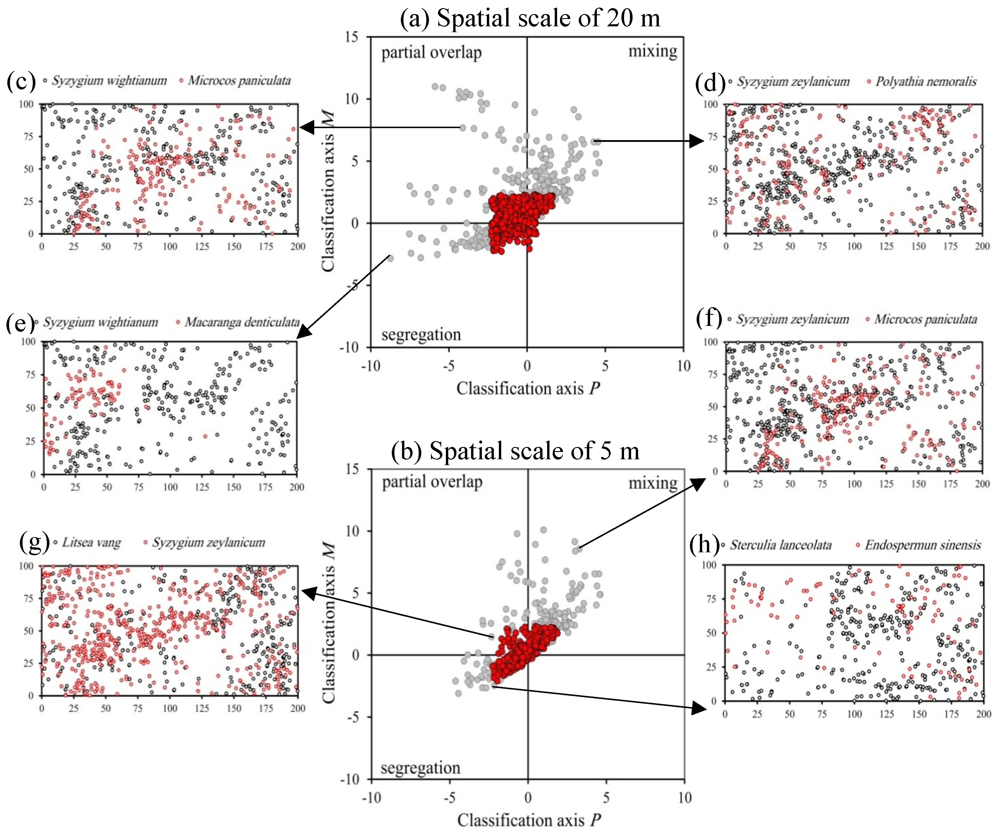
2.2.2. Analysis 2—Overall Interspecific Association Patterns

We employed the technique proposed by Wiegand et al. [13] to reveal the overall interspecific interactions of 18 species which have more than 50 individuals within the study plot. It characterizes the heterogeneous species–species associations by a two-dimensional classification scheme, which is based on the two summary statistics Ripley’s K function K_ij(r) and cumulative nearest neighbor distribution function D_ij(r) [3,31]. The subscripts i and j refer to the spatial patterns of focal species (i) and secondary species (j) which include all possible species pairs. The type of interspecific association detected by the classification scheme can be caused by environmental heterogeneity, interspecific interactions of species i and j, and univariate aggregation of the species.

K_ij(r) shows the expected number of species j within radius r of species i, divided by density of species j and D_ij(r) exhibits the distribution of distances from species i to the nearest species j. These summary statistics explore completely different characteristics of bivariate point patterns and therefore, are able to distinguish different types of species–species associations.

As explained by Getzin et al. [10], high variability and spatial trends of bivariate point patterns may cause contrasting results of K_ij(r) and D_ij(r) and therefore, they proposed an updated version of classification scheme that uses standardized effect size of K_ij(r) and D_ij(r). The two axes of scheme are defined as following:

$$\{\begin{array}{c}P\left(r\right)=\frac{\left(D_{ij}\left(r\right)-E\left[D_{ij}\left(r\right)\right]\right)}{SD\left[{\mathrm{D}}_{ij}\left(r\right)\right]}\\ M\left(r\right)=\frac{\left(K_{ij}\left(r\right)-E\left[K_{ij}\left(r\right)\right]\right)}{SD\left[K_{ij}\left(r\right)\right]}\end{array}$$

(4)

E and SD are expectation and standard deviation of K_ij(r) and D_ij(r) at spatial scale r, respectively, when species i and j are spatially independent. The homogeneous Poisson point process with 199 simulations was applied as the null model in which the spatial locations of species i were kept fixed but the locations of species j were distributed randomly and independently of the spatial pattern of species i. This null model was implemented to explore the significant types of interspecific interactions of the species from those purely happened by chance.

The distribution of P(r) and M(r) is approximately the standard normal distribution, we considered p-value of 0.025 for each axis (i.e., P and M) to reach 5% error rate for both summary statistics. If the amounts of P(r) and M(r) are less than 2.33 and greater than −2.33, the null hypothesis (i.e., independence of species i and j) cannot be rejected at the investigated spatial scale. In addition, the farther away a species pair is located from the defined range, the stronger it departs from independence. The location a species pair is in the classification scheme provides additional information on the type of species-species associations. In addition to independence, there are four types of associations possible for each spatial scale r (

Table 1. Four possible types of species–species associations based on the values of P(r) and M(r) axes of the classification scheme.

Association Type	P(r)	M(r)	Description
Segregation	<0	<0	Individuals of species j occur consistently less around individuals of species i within neighbourhoods with spatial scale r than expected under independence
Partial overlap	<0	≥0	Individuals of species j occur on average more often within neighbourhoods of individuals of species i than expected but a notable proportion of individuals of species i have less individuals of species j at their neighbourhood than expected
Mixing	≥0	≥0	Individuals of species j occur consistently more around individuals of species i within neighbourhoods with radius r than expected
Type IV	≥0	<0	Individuals of species i are highly clustered and few individuals of species j are close to the species i clusters

). We considered the cases that were significantly departed from independence and counted the cases for each type of association and spatial scale. The cases that did not exhibit significant departure from independence were considered as independence type.

The methods described above were implemented by using softwares namely Programita [31], [http://programita.org/] with spatial resolution of 1 m and Crancord (http://crancord.org/). To eliminate the edge effect of the estimates in M_i, W_i and U_i calculation, we applied the nearest neighbor edge correction method proposed by Pommerening and Stoyan [32].

3. Results

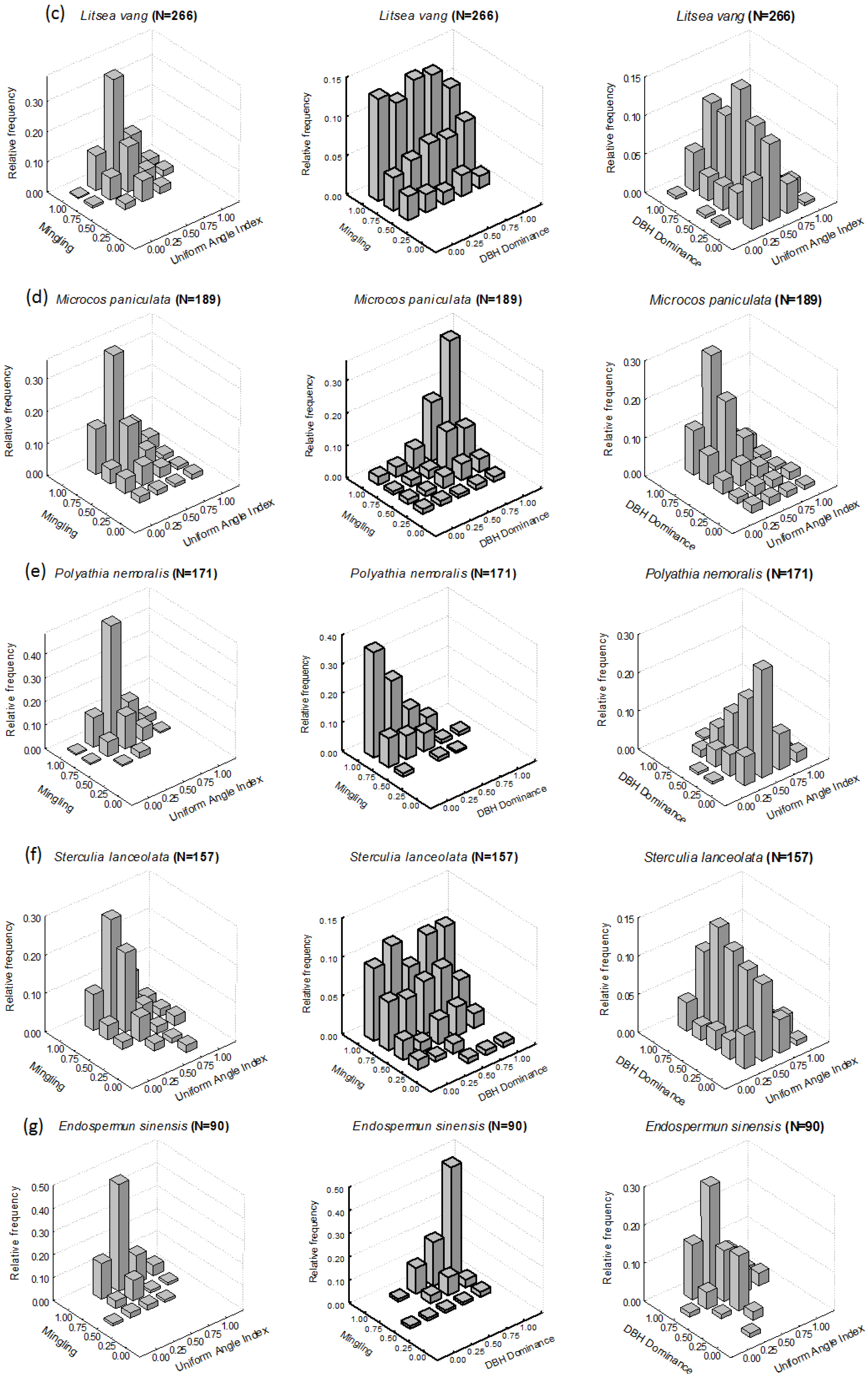
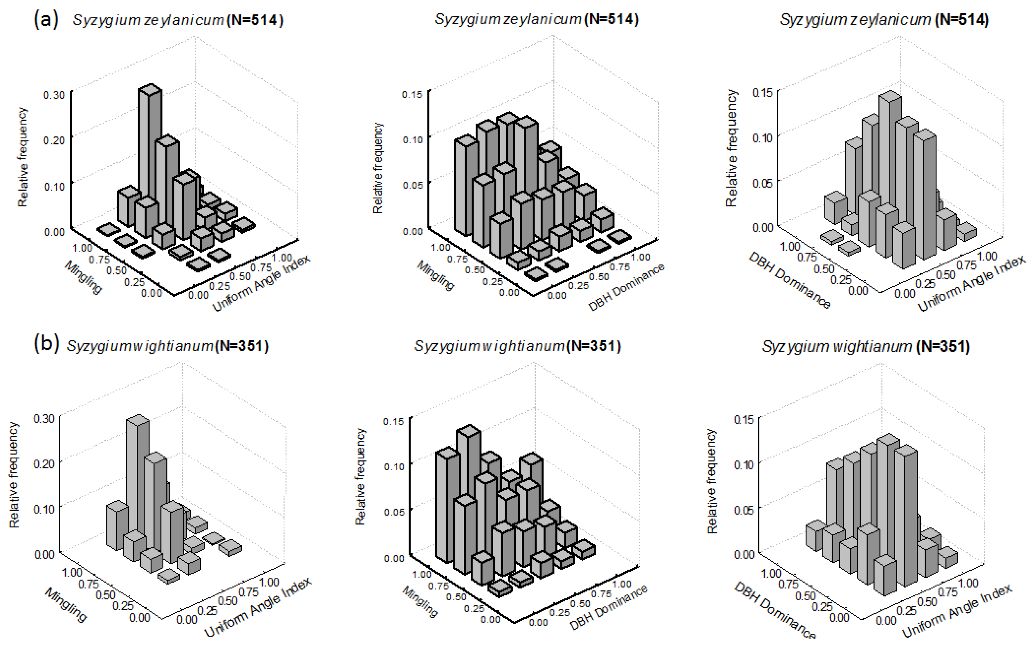
3.1. Intraspecific Patterns

In total, 3154 individuals were investigated belonging to 81 tree species (

Table 2. Characteristics of tree species in the 2-ha plot.

No	Species	N	DBH (Mean ± SD) (cm)	IVI (%)	Mean
					M	U	W
1	Syzygium zeylanicum (L.) DC. *	514	10.05 ± 8.01	10.44	0.77	0.44	0.51
2	Syzygium wightianum Wall. ex Wight & Arn *	351	9.54 ± 7.18	7.35	0.80	0.42	0.52
3	Litsea vang Lecomte *	266	12.30 ± 9.85	7.04	0.87	0.50	0.51
4	Microcos paniculata L. *	189	21.37 ± 6.93	7.07	0.86	0.81	0.50
5	Polyalthia nemoralis Aug. DC. *	171	5.61 ± 2.58	3.39	0.92	0.23	0.51
6	Sterculia lanceolata Cav.*	157	11.94 ± 6.84	4.22	0.80	0.49	0.54
7	Diospyros eriantha Champ. ex Benth.	112	5.33 ± 2.05	2.69	0.93	0.23	0.51
8	Endospermun sinensis Benth. *	90	25.26 ± 10.13	4.76	0.94	0.82	0.49
9	Aphanamixis polystachya (Wall.) R.Parker	81	14.79 ± 11.35	1.95	0.92	0.55	0.52
10	Ardisia lindleyana D.Dietr.	76	14.23 ± 5.90	3.18	0.81	0.67	0.55
11	Macaranga denticulata (Blume) Müll.Arg.	79	3.78 ± 0.72	1.70	0.85	0.14	0.53
12	Schefflera octophylla (Lour.) Harms	71	14.43 ± 11.37	2.67	0.92	0.55	0.48
13	Nephelium melliferum Gagnep.	64	19.53 ± 14.52	4.31	0.94	0.71	0.49
14	Quercus platicalyx Hickel & A. Camus	63	29.96 ± 12.68	3.32	0.91	0.84	0.48
15	Dillenia scabrella (D.Don) Roxb. ex Wall.	62	14.32 ± 11.58	1.74	0.89	0.48	0.51
16	Adina pilulifera (Lam.) Franch. ex Drake	61	8.9 ± 4.93	2.46	0.89	0.42	0.57
17	Archidendron balansae (Oliv.) I.C.Nielsen	54	12.35 ± 6.76	1.98	0.93	0.51	0.52
18	Ormosia balansae Drake	50	29.71 ± 16.42	3.53	0.95	0.86	0.49
19	62 others	643	13.76 ± 10.94	26.11
	All trees	3154	12.53	100

(*) species used in Analysis 1; N- species abundance; DBH- diameter at breast height; SD- standard deviation; IVI- important value index = (relative abundance + relative basal area)/2.

). The forest stand was dominated by 14 medium to shade-intolerant tree species, such as Syzygium zeylanicum, Syzygium wightianum, Litsea vang, Macaranga denticulata, Quercus platicalyx, Dillenia scabrella and Ormosia balansae. Eighteen among 80 tree species having more than 50 individuals were selected for structural analysis of this community. Seven most dominant species, which contribute >40% of total Important Value Index, were taken into analyses of structural indices (Analysis 1), and all 18 species were taken into Analysis 2 about overall spatial association.

3.1.1. M-W Bivariate Distribution

The M-W bivariate distribution of studied species shown a similar trend that most frequency values were concentrated at W = 0.25 to 0.75, have increased gradually from M = 0.25 to 1.00 and had the highest frequency at M = 1.00 (Figure 3). This showed that tree individuals distribute from regularity to clumping and mixture with other species from low to high grades. The other frequency values along with W = 0.0 to 0.25 and W = 0.75 to 1.00 were in very low frequencies. These findings were confirmed by mean values of Mingling and Uniform angle indexes (Table 2).

3.1.2. M-U Bivariate Distribution

The patterns of M-U bivariate distribution were mostly found in two structural combinations (Figure 3). In the first trend, an increasing frequency values extended at grades of DBH dominance from U = 0.00 to 1.00 with increasing grades of Mingling from M = 0.25 to 1.00, containing four species at high abundance such as S. zeylanicum, S. wightianum, L. vang and S. lanceolata. That means, at all levels of DBH dominance, a gradual increase of species mingling reached and was highest frequency value at complete mixture or individual trees are increasingly mixed at all different DBH. The second trend was a single climax, for example cases of M. paniculata, P. nemoralis and E. sinensis. In which, the bivariate M-U distributions were climax at M = 1.00 and U = 1.00 or M = 1.00 and U = 0.00. That means complete mixture of species occurred at absolutely disadvantage of tree size (U = 1.00) or at predominance of tree size (U = 0.00), respectively.

3.1.3. U-W Bivariate Distribution

The U-W bivariate patterns of seven species occurred mainly from W = 0.25 to 1.00 and concentrated at W = 0.50 as highest frequency values, while DBH dominance spread at all grades (Figure 3). From grade of DBH dominance U = 0.00 to 1.00, S. zeylanicum, S. wightianum, L. vang and S. lanceolata were stable at highest frequencies of W; the frequency values increased in cases of M. paniculata and E. sinensis; and decreased in case of P. nemoralis. The findings indicated that, at random distribution of intraspecific trees, DBH dominance could become absolutely disadvantage or highly concentrated in medium or predominance, respectively.

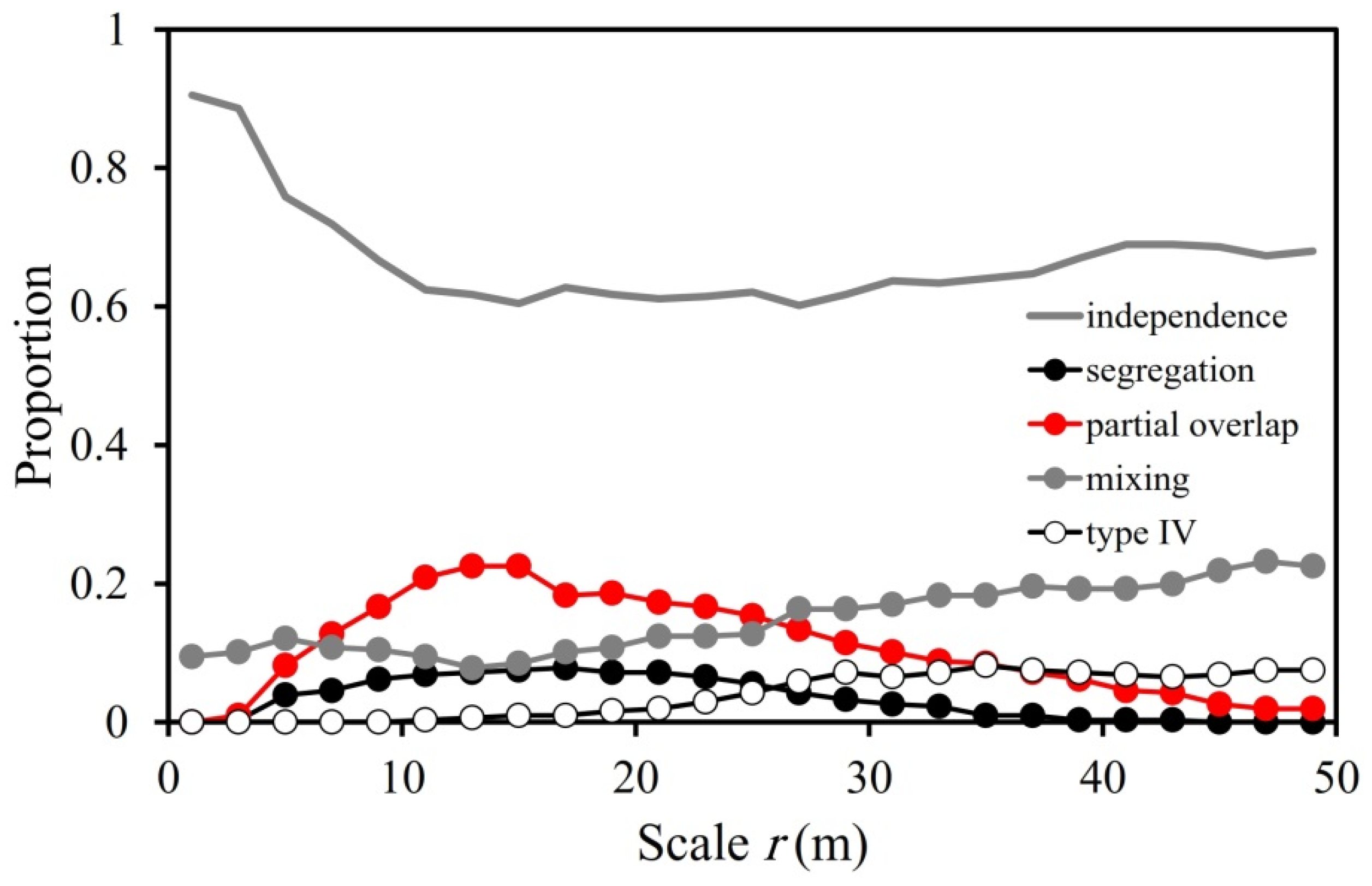
3.2. Overall Interspecific Association Patterns

The overall interspecific association patterns of 18 species were assessed at different spatial scales such as at medium (up to 20 m, Figure 4a), small scales (up to 5 m, Figure 4b), and large scale (up to 50 m, Figure 5), respectively.

At medium and small scales, 306 species pairs analyzed, we found that the most frequent association types were partial overlap of the species (14.6%) up to spatial scale of 20 m and mixing of all species (11.5%) up to spatial scale of 5 m (

Table 3. Summary of interspecific associations of 18 tree species.

Spatial Scales	Types of Association
	Segregation (%)	Partial Overlap (%)	Mixing (%)	Type IV (%)
Up to 5 m	1.4	2.5	11.5	0.0
Up to 20 m	5.5	14.6	10.3	0.5
Up to 50 m	3.5	10.8	15.0	4.0

). No association type IV was observed at both spatial scales, while segregation was the least frequent type up to spatial scale of 20 m (5.5%) and 5 m (1.4%) (Table 3).

The results at large spatial scales up to 50 m showed that the independence between the species dominated in association types, followed by mixing, partial overlap, segregation, and type IV (Table 2). Interspecific independence of 18 species as the dominant association type decreased with increase of spatial scales (Figure 5). Mixing was the most common association type (15.0% of all species pairs) among significant deviations from independence (i.e., segregation, partial overlap, mixing, type IV) at the study plot that was observed at all spatial scales with its peak at scale of 47 m. In addition, mixing was the dominant association type at small (1–7 m) and large (26–50 m) spatial scales. Partial overlap and type IV were the second (10.8% of all species pairs) and third (4% of all species pairs) association types explored within the study plot, respectively, although partial overlap was the dominant association type at spatial scales of 7 m to 26 m with its peak at scale of 14 m.

4. Discussion

The main objective of the study was to carry out analysis of individuals and species associations in both nonspatially and spatially explicit approach. In which, the current techniques based on nearest neighbor distance of events were applied. In Analysis 1, we quantified the forest spatial structure based on the relationship of nearest neighbor tree groups. In Analysis 2, we explored how frequency of species pairs meet and have opportunity to interact. Most of studied species in the forest were highly mixed with other species, while conspecifics were regular to aggregated distributed at small scales. Majority of species–species pairs showed spatial independence (66.7%), whereas 29.8% showed an overall positive association, whereas negative association consisted only a small percentage (3.5%) up to spatial scales of 50 m.

4.1. Intraspecific Patterns

The relationship between tree individuals and their nearest neighbors has potential to elucidate competitive interaction for limited environmental resources, the mutual dependence and species coexistence [24]. The structural parameters were considered closely to species association between each individual and its four nearest neighboring trees by the relationship between mixture, size differentiation and distribution pattern, thus, this approach is advantageous compared to the univariate analysis of structural parameters [33].

Spatially explicit diversity function shown evidences that most of studied species were found in regular to clumped distribution patterns while they were highly mixed with other species. Moreover, species mixture occurred at all DBH dominance levels. These finding may be a reflection of dispersal limitation and development processes of this forest community. The tendency of species aggregation is common and especially in high tree species diversity forests [5], as a pattern of mixed species would lead to a reduction of species diversity due to competitive interaction. This is similar to a finding of Hubbell and Foster [34] that, in species-rich communities, two individual of the same species may share only a few common species among their nearest neighbors. Moreover, functionally similar species may produce ecological equivalence among species traits which was explained by neutral theory [35]. Among 18 studied species of 81 species in this forest community, most are light demanding and inclining to shade intolerance [36], therefore nearest neighbors may have similar ecological requirement revealed via highly spatial mixture. The findings also showed that the spatial structures did not depend on species abundance and were observed at S. zeylanicum or S. wightiamum (high abundance) as well as S. lanceolata or E. sinensis (low abundance). In addition, M. paniculata and E. sinensis contain some large DBH tree individuals, the climax was similarly found in bivariate M–U distribution. This emphasized that complete mixture in species can occur at absolutely disadvantaged stage of DBH dominance. During successional process to climax state, forest community gradually shifts from clumped to regular and the process is constantly accompanied by random weakening of interspecific associations among dominant species [37]. The findings of our study show support for this scenario.

4.2. Overall Interspecific Association Patterns

We found that approximately 66.7% of individuals of 18 species were independent from their heterospecific neighbors, while 15.0% of the species showed positive associations of mixing (approximately 45% of significant deviations from independence), 10.8% partial overlap, 4% type IV (individuals of reference species are highly clustered and few individuals of other species are close to the reference species’ clusters), and only 3.5% negative associations of segregation in their interspecific interactions (approximately 32.5%, 11.9%, and 10.6% of significant deviations from independence, respectively). Our analysis explored that a majority of species exhibited independence from their heterospecific neighbors and the proportion of species pairs showing independence decreased with scale increase (84.5% at small spatial scale of 1–5 m, 69.1% at medium scale of 1–20 m, 66.7% at large scale of 1–50 m). This was in accordance with the results obtained in species-rich forest communities by Wiegand et al. [3] and Wang et al. [17]. They also concluded that the proportion of no association type decreased with spatial scale. Although our study plot had lower richness compared to the dynamic plots (BCI with 303 species, Panama; Sinharaja plot with 205 species, Sri Lanka; CBS plot with 51 species, China), scale-dependent changes in species pairs with no association in a forest plot with low richness were similar to plots with medium or high richness. As revealed by Wang et al. [15] in a plot with 238 species, we also found that the proportion of no association type was not related to species richness. At our study plot with 18 species, 84.5% of species pairs exhibited no association at 5 m scale, while Wiegand et al. [3] explained that CBS plot with the lowest richness (51 species) had the lowest rate of independence among species pairs (36%) at 6 m spatial scale, while BCI plot with high richness (303 species) exhibited higher rate of independence (82%). Moreover, as explained by Wang et al. [17] in species rich communities, stochasticity may govern stronger the shaping of the spatial structure compared to in species poorer forests and leads to approximate independence from their in species neighborhood. Our results partly supported the stochastic dilution hypothesis. In addition, Getzin et al. [10] explained that finding large proportions of species pairs with no association type may be caused by applied tests that are not sensitive enough to explore significant interactions. We attempted to reduce this type of error by using two structurally different summary statistics simultaneously.

The results showed that overall species associations were dominated by positive interspecific interactions of the species (approximately 90% of significant departures from the null model), which suggest that the probability of having individuals of species j at neighborhoods of species i is greater than expected, especially at small- and large spatial scales. This finding strongly supports Janzen-Connell hypothesis. Negative association type among species had the lowest proportion of overall species associations, completely disappeared at a 39-m spatial scale. Prevalence of positive interspecific interactions explored by spatial pattern analysis of overall species associations revealed that species tended to aggregated spatial patterns at small and large spatial scales. This outcome was not in agreement with findings by Wiegand et al. [3] that showed that association types of segregation increased with spatial scale, while it decreased with species richness. Wiegand et al. [3] explained that heterogeneity of physical environment may increase negative interspecific interactions between species with dissimilar habitat associations. In our study plot, heterospecifics tended to form clusters at small and large spatial scales because of importance of intraspecific competition. In addition, previous studies in ecosystems with low richness showed that dominance of intraspecific competition may cause segregation of conspecifics and enhance coexistence of different species [38]. This is in accordance with our observations that suggest that intraspecific aggregation was not strong enough to yield clusters of conspecifics and we explored clusters of heterospecifics, especially at spatial scales of 1–7 m and 27–50 m.

5. Conclusions

The present study extends existing stand-level knowledge on tropical mixed broadleaved forest by investigating species intra- and interspecific interactions, specifically the relationships of nearest neighbors of conspecific and heterospecific trees at fine spatial scales using the indices based on distance to nearest neighbor. Furthermore, for a deeper deciphering of what extent mixing effects (e.g., competition and facilitation between the tree species composing the mixture) govern the dynamics and structure of this forest, overall species associations of heterospecifics were analyzed through a classification scheme based on bivariate cumulative nearest neighbor distribution function and Ripley’s K function.

Our findings provide evidence that most of studied species were found in regular to clumped distribution patterns while they were highly mixed with other species. Moreover, species mixture occurred at all DBH dominance levels. Among 18 studied species of the 81 species in this forest community, most are light demanding and inclining to shade intolerance, therefore nearest neighbors may have similar ecological requirement revealed via highly spatial mixture. Therefore, due to the importance of intraspecific competition, heterospecifics tended to form clusters at small and large spatial scales. In this forest, our analyses showed also that the spatial structures did not depend on species abundance.

A majority of species exhibited independence from their heterospecific neighbors and the proportion of species pairs showing independence decreased with scale increase. As well, the proportion of no association type was not related to species richness. Overall species associations were dominated by positive interspecific interactions of the species, which suggest that the probability of having individuals of species j at neighborhoods of species i is greater than expected, especially at small- and large spatial scales, finding that strongly supports Janzen-Connell hypothesis.

Our study support for the main ecological theories such as dispersal limitation, neutral theory and Janzen-Connell hypothesis. We also found evidence of other effects on spatial association of tree individuals as the stochastic dilution. Due to the crucial role of competition and facilitation between and within species in the dynamics of mixed forests, both bivariate distribution of the structural parameters and spatial point pattern analysis based on nearest neighbor distance should be applied as advantageous approaches in further study for better understanding of population structure, discovering and protecting biodiversity in the future, but also in explaining species coexistence in species-rich forest communities.

References

1. Ricklefs, R.; Miller, G. Ecology; W.H. Freeman: New York, NY, USA, 1990. [Google Scholar]
2. Legendre, P.; Fortin, M.J. Spatial pattern and ecological analysis. Vegetatio 1989, 80, 107–138. [Google Scholar] [CrossRef]
3. Wiegand, T.; Huth, A.; Getzin, S.; Wang, X.; Hao, Z.; Gunatilleke, C.S.; Gunatilleke, I.N. Testing the independent species’ arrangement assertion made by theories of stochastic geometry of biodiversity. Proc. R. Soc. B 2012. [Google Scholar] [CrossRef] [PubMed]
4. Genet, A.; Pothier, D. Modeling tree spatial distributions after partial harvesting in uneven-aged boreal forests using inhomogeneous point processes. For. Ecol. Manag. 2013, 305, 158–166. [Google Scholar] [CrossRef]
5. Wright, J.S. Plant diversity in tropical forests: A review of mechanisms of species coexistence. Oecologia 2002, 130, 1–14. [Google Scholar] [CrossRef] [PubMed]
6. Stoll, P.; Prati, D. Intraspecific aggregation alters competitive interactions in experimental plant communities. Ecology 2001, 82, 319–327. [Google Scholar] [CrossRef]
7. Monzeglio, U.; Stoll, P. Spatial patterns and species performances in experimental plant communities. Oecologia 2005, 145, 619–628. [Google Scholar] [CrossRef] [PubMed]
8. Tilman, D. Competition and biodiversity in spatially structured habitats. Ecology 1994, 75, 2–16. [Google Scholar] [CrossRef]
9. Stoll, P.; Weiner, J. A neighborhood view of interactions among individual plants. In The Geometry of Ecological Interactions: Simplifying Spatial Complexity; Cambridge University Press: Cambridge, UK, 2000; pp. 11–27. [Google Scholar]
10. Getzin, S.; Wiegand, T.; Hubbell, S.P. Stochastically driven adult–recruit associations of tree species on Barro Colorado Island. Proc. Biol. Soc. 2014, 281, 20140922. [Google Scholar] [CrossRef] [PubMed]
11. Janzen, D.H. Herbivores and the number of tree species in tropical forests. Am. Nat. 1970, 104, 501–528. [Google Scholar] [CrossRef]
12. Connell, J. On the role of natural enemies in preventing competitive exclusion in some marine animals and in rain forest trees. In Dynamics of Population; Den Boer, P.J., Gradwell, G.R., Eds.; Pudoc: Wageningen, The Netherlands, 1971. [Google Scholar]
13. Wiegand, T.; Gunatilleke, S.; Gunatilleke, N. Species associations in a heterogeneous Sri Lankan dipterocarp forest. Am. Nat. 2007, 170, E77–E95. [Google Scholar] [CrossRef] [PubMed]
14. Liu, X.; Liang, M.; Etienne, R.S.; Wang, Y.; Staehelin, C.; Yu, S. Experimental evidence for a phylogenetic Janzen-Connell effect in a subtropical forest. Ecol. Lett. 2012, 15, 111–118. [Google Scholar] [CrossRef] [PubMed]
15. Chacón-Labella, J.; Cruz, M.; Escudero, A. Evidence for a stochastic geometry of biodiversity: The effects of species abundance, richness and intraspecific clustering. J. Ecol. 2017, 105, 382–390. [Google Scholar] [CrossRef]
16. Wang, Q.; Bao, D.; Guo, Y.; Lu, J.; Lu, Z.; Xu, Y.; Zhang, K.; Liu, H.; Meng, H.; Jiang, M. Species associations in a species-rich subtropical forest were not well-explained by stochastic geometry of biodiversity. PLoS ONE 2014, 9, e97300. [Google Scholar] [CrossRef] [PubMed]
17. Wang, X.; Wiegand, T.; Kraft, N.J.; Swenson, N.G.; Davies, S.J.; Hao, Z.; Howe, R.W.; Lin, Y.; Ma, K.; Mi, X.; et al. Stochastic dilution effects weaken deterministic effects of niche-based processes in species rich forests. Ecology 2016, 97, 347–360. [Google Scholar] [CrossRef] [PubMed]
18. McGill, B.J. Towards a unification of unified theories of biodiversity. Ecol. Lett. 2010, 13, 627–642. [Google Scholar] [CrossRef] [PubMed]
19. Corral-Rivas, J.J.; Wehenkel, C.; Castellanos-Bocaz, H.A.; Vargas-Larreta, B.; Diéguez-Aranda, U. A permutation test of spatial randomness: Application to nearest neighbour indices in forest stands. J. For. Res. 2010, 15, 218–225. [Google Scholar] [CrossRef]
20. Clark, P.J.; Evans, F.C. Distance to nearest neighbor as a measure of spatial relationships in populations. Ecology 1954, 35, 445–453. [Google Scholar] [CrossRef]
21. Pielou, E. Mathematical Ecology, 2nd ed.; Wiley: Hoboken, NJ, USA, 1977. [Google Scholar]
22. Diggle, P.J. Statistical Analysis of Spatial and Spatio-Temporal Point Patterns; CRC Press: Boca Raton, FL, USA, 2013. [Google Scholar]
23. Ripley, B.D. Modelling spatial patterns. J. R. Stat. Soc. Ser. B. Methodol. 1977, 39, 172–212. [Google Scholar]
24. Von Gadow, K.; Hui, G.; Albert, M. Das Winkelmaß-ein Strukturparameter zur Beschreibung der Individualverteilung in Waldbeständen. Centralblatt für das Gesamte Forstwesen 1998, 115, 1–9. [Google Scholar]
25. Aguirre, O.; Hui, G.; von Gadow, K.; Jiménez, J. An analysis of spatial forest structure using neighbourhood-based variables. For. Ecol. Manag. 2003, 183, 137–145. [Google Scholar] [CrossRef]
26. Hui, G.; Zhao, X.; Zhao, Z.; von Gadow, K. Evaluating tree species spatial diversity based on neighborhood relationships. For. Sci. 2011, 57, 292–300. [Google Scholar]
27. Von Gadow, K.; Hui, G. Characterizing forest spatial structure and diversity. In Sustainable Forestry in Temperate Regions; Materiały Konferencyjne IUFRO: Lund, Sweden, 2002; pp. 20–30. [Google Scholar]
28. Van Laar, A.; Akça, A. Forest Mensuration; Springer Science & Business Media: Dordrecht, The Netherlands, 2007; Volume 13. [Google Scholar]
29. Von Gadow, K.; Zhang, C.Y.; Wehenkel, C.; Pommerening, A.; Corral-Rivas, J.; Korol, M.; Myklush, S.; Hui, G.Y.; Kiviste, A.; Zhao, X.H. Forest structure and diversity. In Continuous Cover Forestry; Springer: Berlin, Germany, 2012; pp. 29–83. [Google Scholar]
30. Pommerening, A.; Gonçalves, A.C.; Rodríguez-Soalleiro, R. Species mingling and diameter differentiation as second-order characteristics. Allgemeine Forst Und Jagdzeitung 2011, 182, 115–129. [Google Scholar]
31. Wiegand, T.; Moloney, K.A. Handbook of Spatial Point-Pattern Analysis in Ecology; CRC Press: Boca Raton, FL, USA, 2014. [Google Scholar]
32. Pommerening, A.; Stoyan, D. Edge-correction needs in estimating indices of spatial forest structure. Can. J. For. Res. 2006, 36, 1723–1739. [Google Scholar] [CrossRef]
33. Li, Y.; Hui, G.; Zhao, Z.; Hu, Y.; Ye, S. Spatial structural characteristics of three hardwood species in Korean pine broad-leaved forest—Validating the bivariate distribution of structural parameters from the point of tree population. For. Ecol. Manag. 2014, 314, 17–25. [Google Scholar] [CrossRef]
34. Hubbell, S.P.; Foster, R.B. Biology, chance, and history and the structure of tropical rain forest tree communities. Community Ecol. 1986, 314–329. [Google Scholar]
35. Hubbell, S.P. Neutral theory and the evolution of ecological equivalence. Ecology 2006, 87, 1387–1398. [Google Scholar] [CrossRef]
36. Nguyen, H.H.; Uria-Diez, J.; Wiegand, K. Spatial distribution and association patterns in a tropical evergreen broad-leaved forest of north-central Vietnam. J. Veg. Sci. 2016, 27, 318–327. [Google Scholar] [CrossRef]
37. Zhang, J.; Chen, L.; Guo, Q.; Nie, D.; Bai, X.; Jiang, Y. Research on changes of dominant tree population distribution patterns during developmental processes of a climax forest community. Acta Phytoecol. Sin. 1999, 23, 256–268. [Google Scholar]
38. Raventós, J.; Wiegand, T.; Luis, M.D. Evidence for the spatial segregation hypothesis: A test with nine-year survivorship data in a Mediterranean shrubland. Ecology 2010, 91, 2110–2120. [Google Scholar] [CrossRef] [PubMed]
Figure 1. Map of study region and location of 2-ha study plot.
Forests 09 00033 g001
Figure 2. Definition of the spatial parameters: mingling (a); dominance (b) and uniform angle index (c).
Forests 09 00033 g002
Figure 3. Bivariate distributions of M-W, M-U, and U-W for most seven dominant species.
Forests 09 00033 g003aForests 09 00033 g003b
Figure 4. Classification of species-species associations at medium and small scales. The grey circles in (a) and (b) indicated significant association types, the red circles showed no significant departure from independence. At medium spatial scale, examples for a partial overlap between S. wightianum and M. paniculata (c); a mixing between S. zeylanicum and P. nemoralis (d); a segregation between S. wightianum and M. denticulate (e). At small spatial scale, examples for a mixing association between S. zeylanicum and M. paniculata (f); a partial overlap between L. vang and S. zeylanicum (g); a segregation between S. lanceolata and E. sinensis (h). In panels (ch), black dots are focal species and red dots are secondary species, three species pairs corresponded to different types of species associations were shown in Figure 4c–h, in which S. wightianum showed patterns of partial overlap with M. paniculata, although this species exhibited segregation association with M. denticulate up to spatial scale of 20 m (Figure 4c,e).
Forests 09 00033 g004
Figure 5. The overall interspecific associations at large scales (For details, see Table 1).
Forests 09 00033 g005