1. Introduction
Although understorey species contain less than 1% of the aboveground biomass of tropical forests in the Northern Hemisphere, they play a critical role in supporting global ecosystem services [
1]. The vast majority of plant species in north-temperate forests and plantations are not overstorey tree canopy but rather understorey herbs, shrubs, and subshrubs [
2]. As a critical component of the forest ecosystem, the understorey layer supports ecosystem floristic diversity, wildlife species, and ecosystem services such as carbon sequestration [
3]. The dynamics of the understorey layer are closely associated with long-term forest successional patterns [
4]. Earlier studies have suggested that forest understorey layers can interact with the overstorey canopy, affect species regeneration [
5,
6], contribute to forest biodiversity, and influence energy fluxes and nutrient cycles [
7].
Within forest stands, differences in vegetation composition, structure, and foliage distribution create spatial variation in light transmittance to the understorey, affecting the growth and mortality of tree seedlings and saplings [
8]. Because canopy structure remains poorly defined at the stand scale, there is a need for ecologists to understand how tree crowns occupy the three-dimensional (3D) space of the canopy layer and how the understorey environment is influenced by canopy structure [
9]. Therefore, the estimation of the composition, structure, and foliage distribution of understorey vegetation is especially important for research on forest ecosystem function and services. Conventionally, information on the forest understorey is obtained through field sampling, which is generally expensive, labour intensive, and time consuming. Further, a variety of ecological applications require data from broad spatial extents that are impossible to acquire using field-based methods [
10].
Light Detection and Ranging (LiDAR) has attracted much attention from the forestry community as a rapid and efficient tool for the estimation of attributes of forest structure from the plot level to a regional scale. LiDAR systems are based on either the ranges or intensities of individual pulse returns or characterisations of the full waveform to characterise forest structure [
11]. LiDAR allows ranging of objects directly by measuring the time between emitted pulses and their reflected returns. It also allows accurate measurement of forest structure from airborne, terrestrial, or spaceborne platforms through forest canopy gaps. Airborne LiDAR (or Airborne Laser Scanning, ALS) and terrestrial LiDAR (or Terrestrial Laser Scanning, TLS) have the potential to characterise the vertical structure of a forest with high-density point clouds at the stand or plot level [
12].
The distribution of vertical foliage can be derived from both ALS and TLS. As an important feature, the foliage profile along the distribution of the forest canopy has been widely used to describe the distribution of the vertical structure of forests [
13]. Since single spectral band LiDAR does not distinguish branches from leaves, the terms canopy height profiles (CHPs) or apparent foliage height profile are often used [
14]. CHPs can be derived from large-footprint, full-waveform LiDAR systems [
15,
16] and small-footprint, discrete return LiDAR systems [
17] as well as TLS data. Mund et al. [
18] investigated the potential of full-waveform, high-density ALS data for the detection and classification of the structure of vegetation. As a key index for characterising vertical and horizontal canopy distribution, including understorey structures, the distribution of leaf area density (LAD) is enabled from ALS measurement [
19]. Tang et al. [
12] explored the potential of airborne waveform LiDAR for mapping vertical and horizontal distributions of leaf area index (LAI), deriving vertical profiles of LAI at 0.3 m height intervals from the Laser Vegetation Imaging Sensor (LVIS) data. TLS offers the advantage of rapidly and precisely measuring the 3D structure of the lower forest canopy and quantifying forest metrics with a high level of detail. Many studies have extracted vertical forest structure characteristics such as forest canopy gap fraction, vertical foliage profile, clumping index, and LAI with TLS data [
20,
21,
22]. Danson et al. [
23] used TLS to measure the distribution of canopy directional gap fractions in forest stands, finding that they were similar between hemispherical photography and TLS data, with equally high precision.
ALS data have been widely used to retrieve vertical and horizontal forest structure parameters over large areas. Nevertheless, ALS does not directly measure complete forest structure, and the canopy components of understorey layers that are occluded by the overstorey may therefore go undetected. Because transmission losses affect echo triggering probabilities and intensity observations, Korpela et al. [
24] formulated a conceptual model to detect losses due to below-the-noise-level backscattering in the understorey. Although neither ALS nor TLS systems can directly provide complete information on forest structure, TLS data can measure forest structure more accurately, especially the canopy understorey [
25]. TLS data can be collected only from limited field plots; however, it can be used to rebuild the 3D forest structure more precisely and provide an approach for calibrating ALS data and improving the accuracy of the estimation of forest structural variables [
26,
27,
28,
29]. Additionally, TLS data provide more spatial details of understorey forest structure than overstorey structure due to the upward-looking data collection method, making it suitable for the calibration and validation of ALS data. Over the past decade, research combining ALS and TLS data for the characterisation of forest structure has improved the detectability of foliage and biomass distribution within the forest canopy. Research utilizing ALS and TLS data from forest environments has been explored in many different fields. For example, Wezyk et al. [
30] integrated ALS and TLS data to retrieve forest inventory attributes such as tree height, diameter at breast height (DBH), basal area, crown closure, crown base height, and 2D and 3D tree crown surface with increased accuracy. Zhao et al. [
31] estimated LAI and vertical foliage profile using a voxel-based method with TLS data and found that there was little difference between vertical foliage profiles retrieved from TLS, ALS, and a field survey. Greaves et al. [
32] compared aboveground shrub biomass derived from TLS and ALS with an
R2 value of 0.62 and found that the accuracy of ALS-derived shrub biomass predictions was the same whether they were calibrated directly against harvest biomass or against TLS-derived estimates of biomass.
Both ALS and TLS have demonstrated their potential in measuring the vertical structure of the forest canopy and the vertical distribution of the understorey layer, and their dynamics have been explored in studies. Previous research has connected CHPs from ALS and TLS layer by layer but has not taken into account overstorey shielding effects. In this study, we explored the potential advantage of linking ALS- and TLS-derived CHPs to assess changes in forest understorey volume before and after forest tending. We used detailed, plot-scale TLS understorey measurements to validate the ALS CHPs that come from both understorey and overstorey. The final objective of this study was to detect understorey changes caused by forest-tending practices in a young Khasi pine forest with a synergistic use of ALS and TLS.
2. Materials and Methods
2.1. Study Area
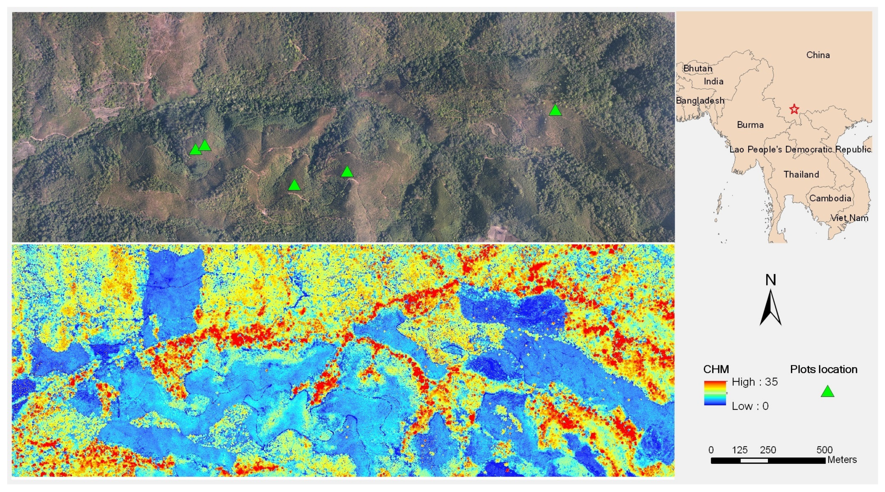
The study was conducted at the Wanzhangshan Forest Farm (
Figure 1; 22°55′09″ N, 100°56′51″ E), located in Yunnan province, China. The main land cover types here are natural mixed conifer and broadleaf forest, natural broadleaf forest, young Khasi pine planted forest, and tea plantations. In the natural forest, the dominant species are Khasi pine (
Pinus kesiya), Schima (
Schima superba Gardner & Champ.) and Quercus glauca (
Cyclobalanopsis glauca Oerst.). The young Khasi pine plantation is managed by the Wanzhangshan Forest Farm, with a very dense layer of shrubs and herbs in the understorey. The Khasi pine trees in the study area are no more than 6 years old, and the shrubs and herbs had never been removed before December 2013. Shrubs and herbs in the young Khasi pine stands compete for nutrients with young Khasi pine trees and are deemed an impediment to the growth of the forest plantation. In December 2013, the Wanzhangshan Forest Farm began to thin the shrub layer as well as dead and unhealthy trees.
2.2. ALS Data Acquisition and Preprocessing
ALS data were acquired in December 2013 and March 2014 with a Yun-12 airplane at an altitude of approximately 1500 m. The sensor used was a RIEGL LMS-Q680i, with full-waveform data acquired [
33]. The raw data were decomposed according to Gaussian decomposition models into discrete returns and georeferenced with position and orientation data. From the statistics of discrete returns in the study area, the minimum and maximum numbers of returns extracted from each waveform were 1 and 4, respectively. The discrete returns dataset thus had a maximum and minimum average point density of 6.5 pts/m
2 and 5.3 pts/m
2, respectively. Ground and non-ground returns were separated with a ground point filter method using the software package Terrascan [
34], and the elevation of LiDAR return points was normalised with respect to the ground points. At the time of the first ALS data acquisition, forest tending in the Khasi pine forest had not yet begun. However, at the time of the second ALS data acquisition, forest tending was ongoing.
2.3. TLS Data Acquisition and Preprocessing
The TLS data were collected using a Trimble TX8 terrestrial laser scanner (Trimble, Sunnyvale, CA, USA) in December 2013 and March 2014. The scanner uses a narrow infrared laser beam with a rapid scanning mechanism that allows rapid and non-contact data acquisition. The detection range was 120 m with a scan duration of 2–14 min. The vertical and horizontal scan angle ranges were 317° and 360°, respectively.
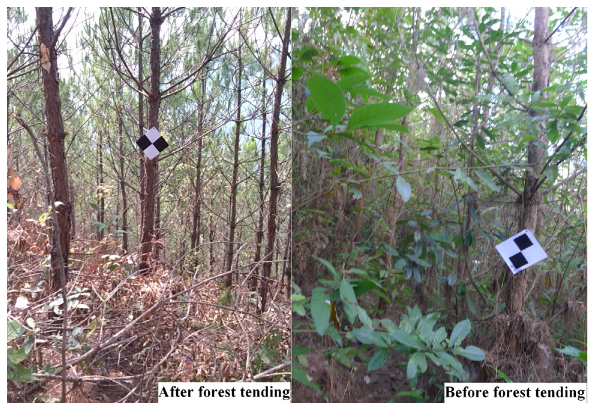
Due to poor visibility in the young Khasi pine forest caused by the density of the shrub layers, it is difficult to set up reference targets to register multiple scan stations, because each target should be detected by all scans. Therefore, all five plots were designed to have only one TLS scan at the plot centre. We located and marked the plot centre using differential Global Positioning System (DGPS). Within each plot, five reference targets (
Figure 2) were used during scanning, allowing us to geo-register the scans using a total station and DGPS. All five targets were posted on stems that were visible to the scanner. All plots were scanned twice: before and after forest tending. The coordinates of the TLS return points were translated by DGPS using the software package Trimble RealWorks [
35]. Ground and non-ground returns were separated with the same method as for ALS data, using Terrascan.
2.4. Plot Description
Due to occlusion by shrubs and leaves before forest thinning, the recognition ability of TLS data decreased with increases in distance between the scanning equipment and the target forest stands. Therefore, we used the return points collected from forest stands within a 5-m buffer of the plot centre to extract CHPs and foliage volume in the understorey.
All young Khasi pine trees in the tending area were of the same age and therefore had very similar DBH and tree height values. When afforestation began, the forest farm planned several stand densities. We located our plots within five different stand densities to collect TLS data. The descriptions of these plots, including manual measurements from TLS data, are shown in
Table 1. For each plot, the TLS scan position was the same before and after forest tending.
2.5. Canopy Height Profiles Extraction
As an active remote sensing technology, the emitted laser pulse from LiDAR can penetrate the upper canopy to reach the understorey or the ground. Given this ability to accurately measure canopy structure, CHPs can be derived from LiDAR point clouds data. Extractions of most forest parameters were based on normalised point clouds to eliminate the influence of terrain on tree height. From the normalised LiDAR point clouds data, canopy height distribution can be divided into different height strata at 0.5 m intervals. Canopy cover within each stratum (z) can then be calculated using the percentile distribution (PD) of point clouds in this stratum, as shown in Equation (1) [
28]. Finally, the CHPs from the ALS data can be drawn from the PD values of all layers:
where PD(z) is the PD of ALS return points at height z from the ground,
N(z) is the number of return points in layer z, and
Ntotal is the number of return points.
Conversely, terrestrial LiDAR collected more than one million return points from one position in the understorey. Due to the high point density and uneven distribution of TLS data, a voxel-based method was used to derive the CHPs of TLS data after the heights of TLS return points were normalised with ground elevation. The voxel method reduced the complexity of TLS data and permitted the characterisation of the vertical distribution of the forest canopy. Voxel size was an important parameter, and it played an important role in CHPs extraction. Large voxel size reduces the amount of canopy structure detail, whereas small voxel size may neglect important CHPs information. García et al. [
36] evaluated the effects of voxel size on the estimation of degree of canopy clumping (Ω) by testing 5–25 cm voxels at 5 cm intervals when using TLS data. Three Ω-estimation methods were tested for different zenith ranges. The correlation values yielded by three Ω-estimation methods for different zenith ranges and voxel sizes were examined. Chen and Cihlar’s clumping index (CCI) [
37] for the 55–60 zenith range and a 5-cm voxel size yielded the strongest correlation between TLS-derived Ω and validation Ω extracted from hemispherical photographs. In that study, the 55–60 zenith range was the highest zenith range. Cifuentes et al. [
38] inspected the effects of voxel size (ranging from 1 cm to 5 cm) and sampling design on the estimation of the forest canopy gap fraction using TLS data. The root mean square error (RMSE) of gap fraction estimates for intermediate and mature forests using point clouds at different locations (1 m, 10 m, and 14 m from the centre) decreased as voxel size increased. There was little difference in the RMSE of gap fraction estimates using point clouds at different locations from the scan centre with a 5-cm voxel size. To detect understorey volume, we used return points with larger zenith ranges. Consequently, a 5 × 5 × 5 cm voxel size was selected to extract TLS-derived CHPs with a height interval of 0.1 m from the ground to the top of the canopy. Voxels that contained more than 10 return points were designated filled voxels.
2.6. Understorey Volume Estimates and Changes Detected after Forest Tending
The main objective of forest tending was to remove shrubs, grasses, and unhealthy or dead trees. Because the height of the TLS scan station was approximately 1.5 m, it more precisely detected the understorey than the overstorey. To estimate understorey volume and detect any change in volume after forest tending in the young Khasi pine forest, CHPs were separated into ground, overstorey, and understorey layers according to the CHPs before and after forest tending.
Because most materials removed after forest tending were in the understorey, the variation of CHPs referred to the change of understorey distribution. A threshold height was chosen to separate understorey and overstorey according to the variation in all CHPs in this study. The threshold height was the height below which substantial material was removed and above which material was rarely removed. After forest tending, all removed material was piled on the ground to a height of approximately 0.5 m. For this reason, we defined 0.5 m as the threshold height for separating the ground and understorey layers. Therefore, the ground layer included grasses and short shrubs as well as bare ground before forest tending and shrub debris after forest tending.
The understorey volume, calculated using the number of filled TLS voxels, was considered the reference value. The change in understorey volume was calculated from the understorey volume before and after forest tending.
ALS-derived PD of the overstorey and understorey layers were calculated to compare to the TLS-derived understorey volume. We used two methods to compare the understorey volume according to TLS and the PD according to ALS. First, we directly compared the PD values according to ALS from the understorey (Equation (1)) with the understorey volume according to TLS. However, the detectability of understorey PD values from ALS was heavily impacted by the shading effects of the overstorey. In addition to the greater numbers of branches and leaves in the overstorey, higher PD values for the overstorey also indicated stronger shading effects. PD values for the z layer were related to the amount of branches and leaves in this layer and in the overstorey canopy cover (above the z layer). Therefore, we used a weighted PD value to compare that of the understorey volume in TLS (Equation (2)):
where PD (h > z) is the PD of ALS return points above height stratum z, or the degree of canopy closure above height z.
Within canopy height distribution in the understorey, the PD from ALS and weighted PD from ALS were expressed as follows:
where the PD values are calculated using ALS return points.
H is the threshold height that separates the understorey and overstorey layers in all plots.
NFilled-Voxel is the number of filled TLS voxels.
Because all five field plots were scanned by ALS and TLS before and after forest tending events, 10 ALS–TLS data pairs were extracted from the field plots. The model was developed from the relationship between the TLS-estimated volume and ALS PD values or weighted understorey PD values for the 10 ALS–TLS data pairs, and leave-one-out cross-validation was performed to evaluate model performance. For each cross-validation split, one sample was tested, using the predictor model derived from the nine remaining samples. The cross-validated coefficient of determination (R2) and RMSE were calculated. Volume changes in the understory after forest tending in the young Khasi pine forest area were calculated based on the model built from all 10 samples.
4. Discussion
Canopy structure is a fundamental property of forest ecosystems. Canopy structure can influence microclimate, runoff, forest disturbance, and biodiversity. A traditional approach to quantifying the canopy vertical structure is to map and measure trees by species, vertical stratification, and canopy class through manual fieldwork [
39]. To determine the distribution of forest canopy cover among strata of forest height, field surveys are quite appropriate to assess canopy vertical structure measurements; however, they are also labour-intensive, scale-dependent, and time-consuming. Remote sensing data and techniques, especially LiDAR, have been used to characterise forest canopy vertical structure from the plot level to regional scales [
40]. However, as part of forest canopy structure, the understorey has rarely been well explored.
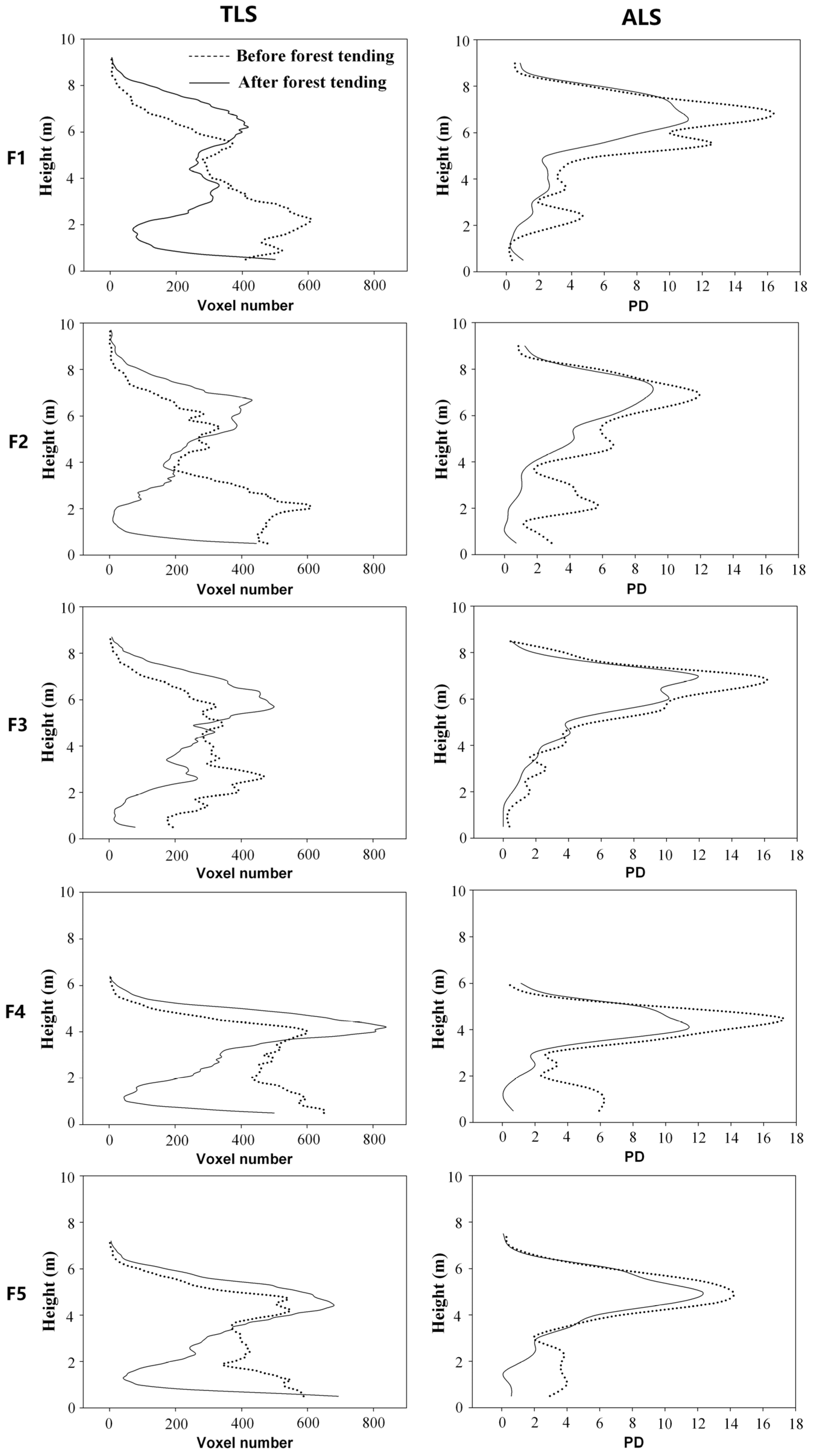
We explored the relationship between ALS- and TLS-derived CHPs in the understorey. ALS- and TLS-derived CHPs of all plots before and after forest tending were extracted.
Figure 3 shows that TLS observations have the advantage of characterising more details in understorey vegetation than in the overstorey. By contrast, ALS-derived data collectively can describe canopy height distribution in the overstorey better than TLS observations, whereas the vegetation components in the understorey are illustrated with less detail. A study by Hancock et al. [
41] yielded a result that our study supports, that TLS-derived vegetation density at the canopy top was underestimated compared to that derived by ALS. Chasmer et al. [
29] examined the voxel column PD at the plot level for ALS and TLS. That study demonstrated that for ALS, a high percentage of laser pulses was intercepted by the top of the canopy with fewer returns from within the canopy and understorey; similarly, for TLS, a high percentage of laser pulses were intercepted by the understorey, stems, and lower canopy, with a lower percentage of pulses reaching the upper canopy. This study and previous research has shown that both ALS and TLS data can represent the vertical distribution of the forest canopy, while also showing the inability of ALS data to characterise understorey vegetation structure in detail. It is meaningful to use TLS data to validate ALS understorey vegetation structure estimates, because TLS shows much more understorey detail than ALS.
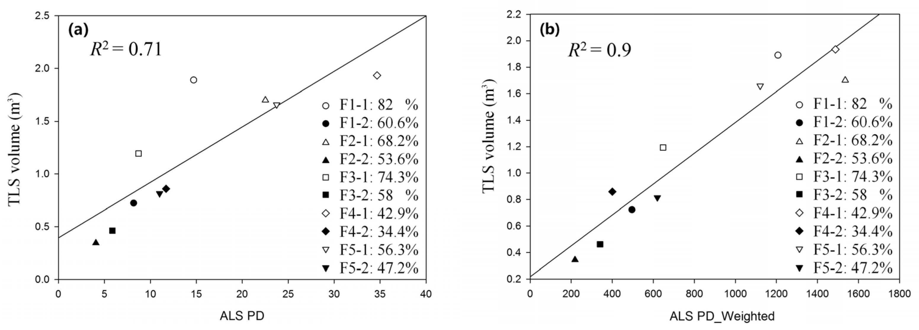
For most plots, the understorey volume was underestimated before forest tending compared to post-forest tending, due to the removal of dead or stressed trees. Because the crowns of removed trees were piled on the ground, more laser points penetrated the overstorey to reach the understorey. Although CHPs from both TLS and ALS were incapable of representing the complete vertical structure of the canopy due to occlusion, the canopy component within one layer was extracted by ALS and TLS data with a high coefficient of determination (R2 = 0.71).
In previous research, the relationship between ALS- and TLS-derived CHPs has been examined without considering the overstorey [
28,
30]. In this study, we combined the PD values for return points in the overstorey and understorey. The relationship between ALS- and TLS-derived canopy component distributions in the understorey became stronger, with the R
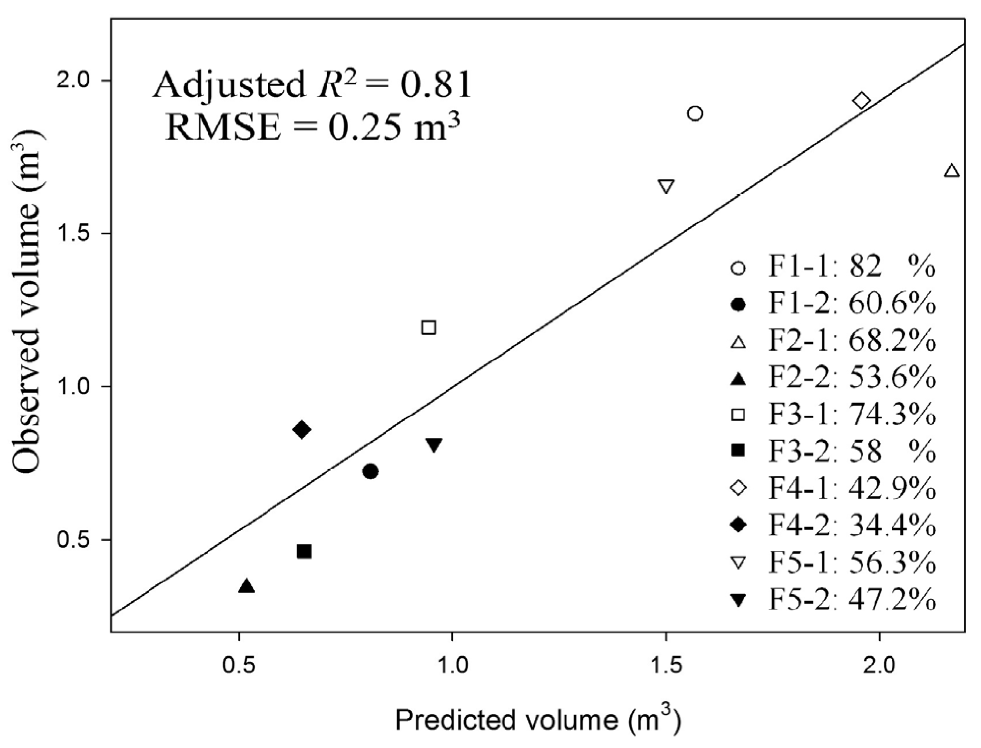
2 increasing from 0.71 to 0.90. Linear regression was performed and an assessment using leave-one-out cross-validation showed an excellent result, with an adjusted
R2 and RMSE of 0.81 m
3 and 0.25 m
3, respectively. This result is important, because it illustrates the capacity of ALS and TLS data to be used for volume estimation in the understorey.
We used the estimated canopy volume to detect variation in the volume of foliage in the understorey. We did not design an experiment to evaluate the relationship between TLS-derived volume and field harvest biomass. In our estimation of the canopy volume of the understorey using ALS data, the volume of the canopy component estimated with filled TLS voxels was used as verification data. Traditionally, ALS data are calibrated against field data to estimate aboveground biomass. To calibrate the biomass of shrubs in the understorey, destructive harvesting is a simple method; however, destructive harvesting is limited by multitemporal and multiscale sampling. TLS provides a potential alternative approach for the calibration of ALS data without destructive harvesting [
23,
31]. Greaves et al. [
42] showed that TLS-derived canopy volume provides a robust proxy to shrub biomass in Arctic tundra. In one of their other studies, aboveground shrub biomass was derived by both ALS and TLS data [
32]. In that study, TLS produced more accurate predictions of shrub biomass (
R2 = 0.78, validated by harvested sampling) than did ALS; however, the accuracy of ALS-derived shrub biomass predictions (
R2 = 0.62) was identical when calibrated directly against harvested biomass and TLS-derived estimates of biomass. The authors suggested that once the initial TLS–harvest relationship was known, TLS could provide validation data for ALS shrub biomass estimation without additional destructive harvesting. Few harvesting samples are needed in specific areas to provide validation data for vegetation structure estimation of the understorey by TLS. Therefore, TLS data have the potential to provide validation data for ALS understorey vegetation structure estimates at regional scales without harvesting samples.
It was difficult to set up multiple TLS scans in the young Khasi pine forest due to the dense understorey shrub layer. Despite this obstacle, there was strong agreement between CHPs from ALS and TLS derived from a single scan in the understorey. Multiple-scan TLS data can describe understorey structure in greater detail. TLS would thus constitute a better validation tool in forested areas where setting up multiple TLS scans is easier. For example, Li et al. [
43] used multi-scan TLS-derived shrub biomass to calibrate a biomass prediction model of ALS-derived percent vegetation cover with a better validation result (
R2 = 0.87) than obtained in this study (
R2 = 0.81).
Our method applied estimates of understorey volume under different ALS point densities using a full-waveform system. Both ALS data showed strong agreement with TLS data. Point density was generally related to the ability to estimate forest structure, with high-density ALS data having greater potential to extract forest structure. However, this argument is not appropriate for ALS data from different sensors, such as discrete-return and full-waveform LiDAR. Discrete-return LiDAR uses proprietary algorithms to produce point clouds and can be biased over vegetation [
44]. Full-waveform LiDAR measures the reflected laser intensity as a function of range, which can depict the full dimension of the target objects [
45]. This study estimated understorey volume and its changes due to forest tending. Unlike discrete-return LiDAR, full-waveform LiDAR offers the potential to measure understorey structure at the resolution of ALS footprint density. The CHPs-based method may not be appropriate for understorey volume estimation using discrete-return LiDAR data (especially first return only) with low-density points in forests with dense canopy cover.
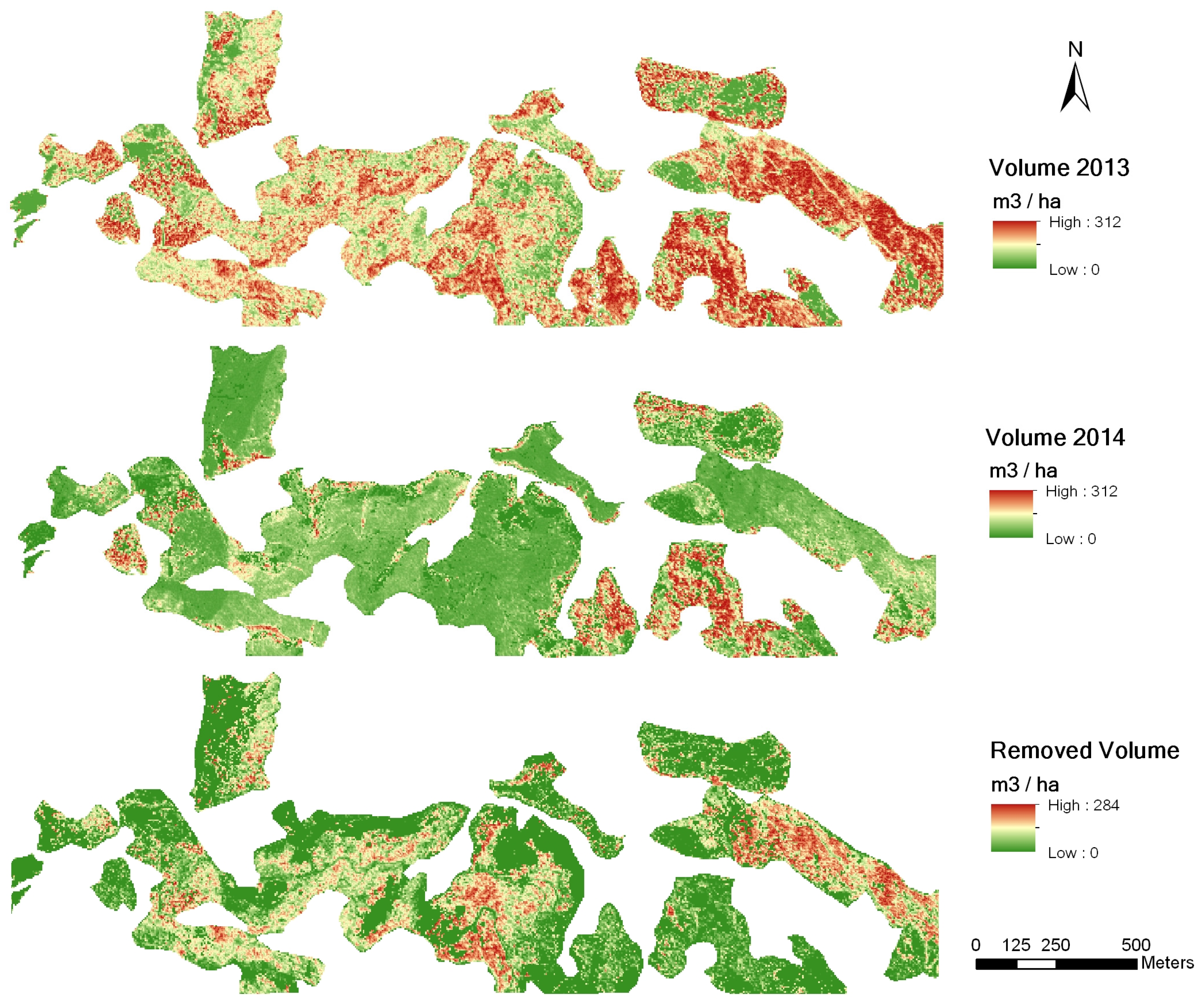
The methods used in our study have great potential for monitoring forest understorey dynamics before and after forest tending activities. The removal of understorey volume due to forest tending can be quantified based on the model developed from TLS and ALS data. In contrast to fine-scale, detailed examination of understorey structure using the TLS technique, ALS remote sensing has the advantage of broad-scale assessment of CHPs over larger areas. Furthermore, ALS data provide greater credibility in quantifying overstorey PDs of return points. Our study found that differences in overstorey canopy cover influenced the understorey volume estimate from ALS data. This finding could help improve the accuracy of ALS-based understorey volume detection by integrating the overstorey canopy cover into the modelling process. It could also improve the development of data collection, specification, and calibration of ALS-derived understorey height distributions through ALS. Shrub and grass cover in the forest understorey plays an important role in forest ecology by providing significant wildlife habitat, modifying soil nutrient cycles, and contributing to forest carbon sequestration. An accurate quantification of disturbance in understorey shrub and grass layers has significant implications for forest diversity and the modelling of forest growth, stand development, and forest succession [
46].


