Abstract
Airborne laser scanning (ALS) based stand level forest inventory has been used in Finland and other Nordic countries for several years. In the Russian Federation, ALS is not extensively used for forest inventory purposes, despite a long history of research into the use of lasers for forest measurement that dates back to the 1970s. Furthermore, there is also no generally accepted ALS-based methodology that meets the official inventory requirements of the Russian Federation. In this paper, a method developed for Finnish forest conditions is applied to ALS-based forest inventory in the Perm region of Russia. Sparse Bayesian regression is used with ALS data, SPOT satellite images and field reference data to estimate five forest parameters for three species groups (pine, spruce, deciduous): total mean volume, basal area, mean tree diameter, mean tree height, and number of stems per hectare. Parameter estimates are validated at both the plot level and stand level, and the validation results are compared to results published for three Finnish test areas. Overall, relative root mean square errors (RMSE) were higher for forest parameters in the Perm region than for the Finnish sites at both the plot and stand level. At the stand level, relative RMSE generally decreased with increasing stand size and was lower when considered overall than for individual species groups.
1. Introduction
Airborne laser scanning (ALS) based forest inventory has been in operational use in Nordic countries for several years [1,2]. Current operational applications are based on an area-based method developed in Norway in 1997 [3] and developed further by Finnish researchers [4,5] to meet the requirement that the inventory results should contain estimates for species distribution in mixed species stands. The approach uses application of the k-nearest neighbor (k-NN) method or Bayesian regression [6] and uses aerial images as additional data to improve the species estimates. Unlike the method presented in [2], the Finnish application does not include pre-stratification based on main tree species or forest development class. However, in practical work, the inventory area is usually selected so that it comprises only one vegetational zone and rather similar forest types. In addition, young stands and mature stands are usually stratified based on tree height and inventoried separately. The method is used in Finland to estimate mean forest characteristics by the most common species groups, namely pine and spruce. Broad-leaved species, which represent only about 10 percent of the total volume, are grouped in one class.
LiDAR (Light Detection And Ranging) was used in Russia for investigation of forest inventory already in the 1970s and 1980s, before the introduction of airborne laser systems [7,8,9], and after a hiatus during the turbulent 1990s, research of the technique resumed in the early 21st century [10,11]. Despite the long history of research in the area, no operational ALS-based method has been developed for large-scale Russian forest inventory and auditing.
This study aims to test the performance of the standard procedure applied in Finland in a large-scale management level forest inventory operation in the Perm region, Volga Federal District, Russia. Large scale in this context means forest area of several thousand hectares, and management level forest inventory means that the results should be accurate at forest stand level, which can be considered as the smallest operational forest unit, i.e., an area of a few hectares or less. The inventory data should be sufficiently accurate to support decision-making about forest operations, for example, timing of thinning or clear-cutting, for an individual forest stand. Additionally, the inventory should fulfill the quality criteria set by forest management authorities.
The Finnish Forest Centre has published forest resources data quality criteria [12]. For inventory purposes, criteria are set for total mean volume (m3/ha) (V), basal area (m2/ha) (G), mean tree diameter (cm) (D), and mean tree height (m) (H). The stand level criteria are set so that in 80% of the stands, the estimates should not exceed the error limits: ±20%, ±3 m2/ha, ±3 cm, ±2 m for V, G, D and H, respectively. Additionally, identification of the main tree species should be correct in cases where there is a clear dominant tree species in a stand. Age and number of stems per hectare (N) are not included in the Finnish Forest Centre quality criteria.
The data quality is controlled by plot level leave-one-out validation results produced by the company submitting the inventory results and by independent stand level control measured by the Finnish Forest Centre. The stand level control is usually done at the so-called micro stand or segment level. Such micro stands are considerably smaller than normal operational forest stands (mean size of micro stand <1 ha). Data quality is also checked at operational stand level by ocular assessment.
The method used in Finland [1] is able to meet the above-mentioned quality criteria in Finnish conditions. In this study, however, the Finnish operational method is applied to new inventory conditions, i.e., conditions in the Perm region in the Urals. Consequently, further research and development may be needed to improve the method and ensure its suitability for Russian conditions and requirements.
The input data for the ALS-based method considered here is sparse point density ALS data, aerial images or equivalent optical multispectral data and field calibration plots. The number of field calibration plots for one inventory area is 600–800 plots for an average inventory area of over 100,000 hectares [12]. The method produces inventory results in two congruent layers: grid and stand. In the area-based method, the basic inventory unit is a cell of a regular grid. The area of each cell is 16 m by 16 m, which corresponds to the size of the field calibration plot. The stand level results are produced by aggregating the results from grid cells to the stand. The grid approach makes it possible to re-calculate the inventory results for any geometry. For example, if stand borders change, the inventory results can be calculated for the new stand geometry from the original grid.
In this study, the ArboLiDAR inventory tool kit developed by Arbonaut Ltd. was used for inventory calculations [13]. Forest parameter estimates in the ArboLiDAR tool kit can be computed with several different regression methods. The method used to compute these estimates in the current experiment is Sparse Bayesian Regression (SBR) [6,14]. Sparse Bayesian Regression is a modified linear regression method that automatically selects the covariates used to estimate each forest parameter. Thereby it also selects the number of covariates automatically. In the basic form of SBR, a different set of covariates is used for each forest parameter.
Linear regression, often called Ordinary Least Squares (OLS), has two main advantages over nearest neighbor methods such as k-NN and k-Most Similar Neighbor (k-MSN). Firstly, unlike nearest neighbor methods, a linear regression model is able to produce estimates beyond the range of parameters present in the training set. This property is particularly valuable for producing estimates over large forest areas in poorly accessible forests, as is often the case with remote forestland. Secondly, linear models can be made accurate with a substantially smaller number of field plots than nearest neighbor models. This effect becomes more pronounced as the number of different forest parameters to be estimated increases, e.g., when parameters pertaining to multiple tree species are required [15,16]. If the training set from the forest has been collected by simple random sampling or some other sampling design that is unbiased by design, the estimates produced by SBR also have this property, i.e., they are asymptotically unbiased when the field sample grows in size. In practice, estimates calculated with SBR have very small systematic errors already with small sample sizes [6]. Further benefits in terms of efficient use of a small number of sample plots and faithful reproduction of forest properties can be attained by using refinements such as Bayesian Principal Component Regression (BPCR) [16,17] but these methods have not yet been incorporated into the ArboLiDAR tool kit.
The aims of this study are to test the ALS-based forest inventory method developed for Finnish conditions in the Perm region, Russia, and compare the results with results reported from Finnish study sites. For this reason, we concentrate on the main timber related forest parameters estimated in Finland, which are mean volume (V, m3/ha), basal area (G, m3/ha), stem count per hectare (N), mean tree diameter (D, cm) and mean tree height, (H, cm). D and H are calculated as basal area weighted means. The estimates are produced for tree species groups and totals. Tree species groups are pine, spruce and broadleaved species. In addition, main tree species classification accuracy and age estimation are considered, because they are important forest parameters in Russia, although they are not of main interest in the comparison. In discussion, we consider possible research needs to adjust the method to Russian conditions.
2. Materials and Methods
2.1. Study Area
The Solikamsk forest district (lesnichestvo) is located in the northern part of the Perm region (Perm Krai). The total area of the district is 510,573 hectares. The length of the forest area from north to south is 72 km, and from west to east 132 km. In total, the Solikamsk forest district includes six regional forest subdivisions. The study area is located in the Solikamsk district in the former Polovodovsky regional subdivision, and it is represented as a square of 10 × 10 km, where the village Polovodovo is located roughly in the middle.
The area of the Solikamsk forest district belongs to the taiga forest vegetation zone of the West Ural taiga region of the Russian Federation. These forests are characterized by a simple forest structure; the shrub layer is absent or is poorly developed and grass-shrub and moss layers are well-developed. Nemoral elements are almost entirely absent. Within the West Ural taiga region, two sub regions are well recognized—one with a dominance of Nordic pine and spruce forests, and the other with a dominance of Kama-Pechora-Zapadnouralskih fir-spruce forests. Forest cover of the Solikamsk district is about 85%. According to forest inventory data from 2007, the study area is mostly occupied by pine and spruce stands, 42% and 34%, respectively. Birch stands occupy 20% and aspen 4% of the stands. The most represented forest types in the area are pine green moss stands (sosnyaki zelenomoshnie) (32%), sorrel spruce stands (elniki kislichnyaki) (21%) and spruce green moss stands (elniki zelenomoshnie) (17%). Bilberry pine forest (sosnyak chernichnik), pinewood sphagnum stands (sosnyak sphagnovii), sedge-sphagnum pine stands (sosnyak osokovo-sphagnovii), polytric pine forest (sosnyak dolgomoshnik) and wet valley spruce forest (elnik log) together comprise 27% of the total area. Deciduous forest types such as birch and alder occur over 3% of the total area.
The tree layer of pine green moss stands is dominated by Pinus sylvestris with an admixture of Picea obovata, Betula pendula, Betula pubescens, Populus tremula, Abies sibirica, Larix sibirica and Pinus sibirica. The tree layer of sorrel spruce forests is usually formed by Picea obovata with an admixture of Betula pubescens, Betula pendula and Populus tremula. Alnus incana occurs rarely with the fraction of Abies sibirica and Pinus sibirica. The green moss spruce stands are dominated by Picea obovata and hybrid forms with Picea abies. Betula pendula, Betula pubescens and Abies sibirica can be quite common and Populus tremula and Pinus sylvestris occur as minor species. The forests in the study area are classified as high-productivity forests with a dominance of high yield stands (Ia–II yield class) and mid-yield stands (III–IV). Low-yield stands (V–VA) represent less than 1% of the area. Based on the relative basal area (otnositelnaya polnota), the forests are dominated by medium stocked stands (srednepolnotnie) (relative basal area 0.6–0.8): 89% of the stands. Fully stocked stands (visokopolnotnie) (relative basal area 0.9–1) and low-stocked stands (nizkopolnotnie) (relative basal area 0.5 and lower) represent 5% and 6%, respectively. Stands are well supplied with undergrowth (podrost) on most of the territory. The average density is around 3000 stems per hectare. The understory (podlesok) is generally sparse.
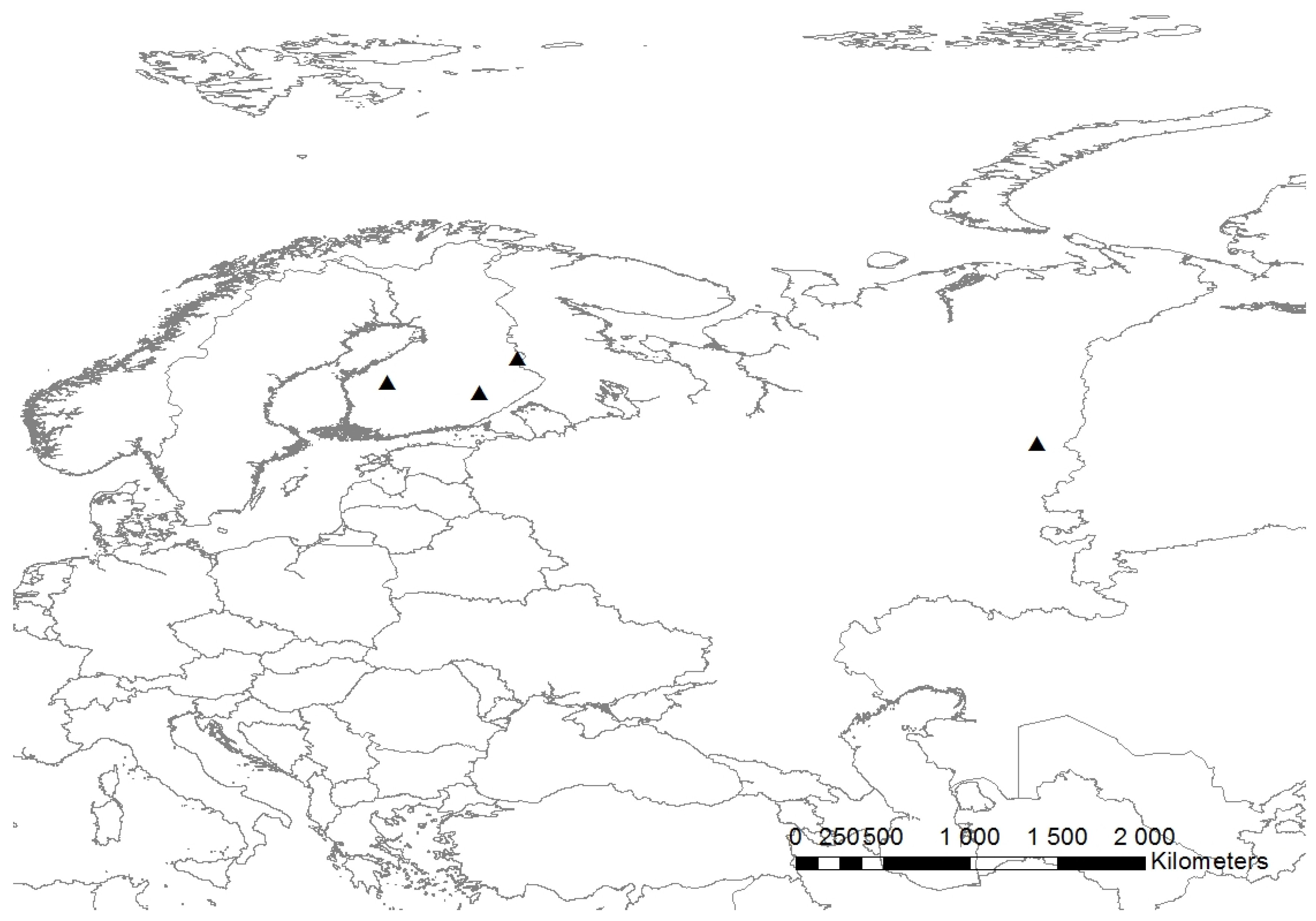
The location of the Perm study site together with the Finnish study sites are presented in Figure 1.
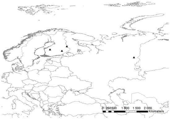
Figure 1.
Location of the Perm study site and the Finnish study sites marked with black triangles. Background map data source and copyright DeLorme/Garmin Ltd. and Esri.
2.2. ALS and Satellite Data
Input data included sparse point density ALS data with a planned nominal point density of 4 points per m2, SPOT 5 satellite images, field reference data (field sample plots) and an existing stand database.
ALS data were acquired in November 2013 with a Leica ALS70 CM laser scanner. The flying altitude was 900–1000 m above ground level. The received point density of the ALS data in the study area was 3–4 points per m2. ALS data were pre-processed by the data vendor and provided in .las format in the WGS84 coordinate system. Provided ALS data were filtered so that error points were removed and the remaining observations were classified in two classes: ground and other points. The ground classification was done with a triangulated irregular network (TIN) based algorithm. The surface adapts to the points and new points are added only if they meet certain data derived threshold parameters. Parameters are derived from the data and they change during the filtering process. In an iterative process, a coarse TIN consisting of initial seed points is densified. The process is described in detail in [18]. The processing of the data and digital terrain model (DTM) with 1 m pixel size was generated from the point cloud data using Terrasolid’s Terrascan software. ALS data were then height-normalized so that the ground level has a height 0 and all heights describe the height from the ground level. This was done by subtracting the DTM from the orthometric heights.
SPOT 5 satellite data were acquired on 7 August 2014. The preprocessing level was 1A. The spatial resolution of the panchromatic band in the SPOT 5 images is 2.5 m and for multispectral images 10 m. Geometric correction for the original imagery was done using reference points, which were taken from very high resolution image fragments. The resulting spatial resolution of the geometrically corrected images was 10.7 and 2.7 m for multispectral and pan-sharpened images, respectively.
2.3. Field Reference Plots
The sample design used mimics the sampling used in Finland by Finnish Forest Centre [19]. The aim of the sampling is not to get a statistical sample, but a representative sample of all forest types and development stages (young, developing, mature) in the whole inventory area. In the Finnish Forest Centre’s sample design, an existing database is used to derive information on main soil class (heathland or peatland), main tree species, basal area and mean diameter. An iterative algorithm is used to get a representative sample that covers the variation in the inventory area. Cluster sampling is used to make the field campaign more efficient. The Finnish Forest Centre’s sampling method was developed in co-operation with Luke, Natural Resources Institute Finland (formerly Metla, Finnish Forest Research Institute) and has some characteristics of the Finnish National Forest Inventory sample design.
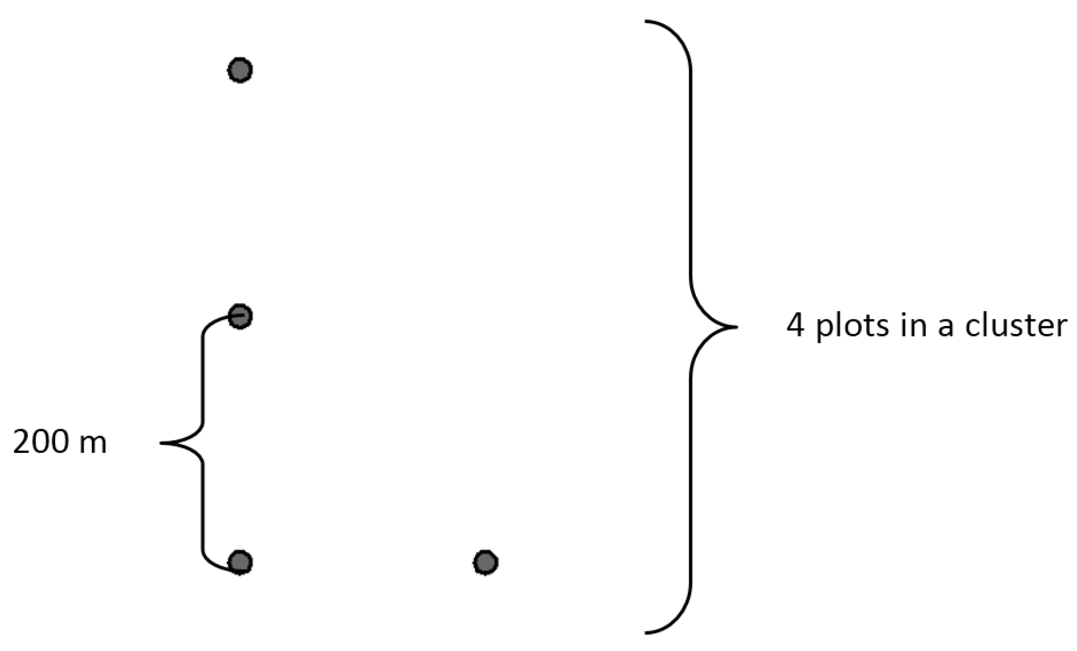
In this study, the sample design was adjusted for the available data using forest type information from an existing stand database and deriving development class information directly from ALS heights instead of the stand database. The initial number of forest types in the study area was 18. The initial forest type classification is based on main species and fertility. The forest types were grouped in seven classes: three pine classes with different fertility, three spruce classes with different fertility, and one deciduous species group. The cluster design was adjusted from nine plots per cluster used in Finland to four plots per cluster because of the relatively small and scattered inventory area. Distance between the plots was set to 200 m as a compromise between avoiding spatial autocorrelation and minimizing field data acquisition costs. Plots within a cluster are in “L” shape, see Figure 2. The field plot size was set to 9 m fixed radius circular plot, which is the same as used in Finnish Forest Centre’s sampling.

Figure 2.
Plot layout in a cluster of four plots.
Clusters that were very close to each other were removed using minimum distance of 700 m between cluster centers as the removal criterion. This distance ensures that the clusters are not overlapping. Height metrics based on ALS data were used to analyze whether the plots were located in a forest or in a treeless, non-forest area. Plots that were located in treeless areas or in areas outside the study area were removed. This allows for more efficient field work because field crews only visit areas relevant to this project. In addition, clusters that ended up having only one plot were also discarded. The initial sample had 308 plots.
2.4. Plot Level Models
The plot data were measured between summer 2015 and autumn 2016. During the field campaign, diameter at breast height (DBH) was recorded for each tree with DBH at least 6 cm (tally trees). Smaller understory trees were also measured but these were not included in the research data. Heights were measured only from height sample trees. The height sample trees were chosen from the tally trees as the basal area median tree of each species. In addition to the basal area median tree, a tree smaller than the median tree and a tree larger than the median tree were selected as height sample trees, i.e., a maximum of three sample trees are measured per species. In total, 24.7% of all measured trees were measured as height sample trees. Age was determined for selected height sample trees to estimate the average forest age.
Calculation of estimated forest parameters from the field measurements was done by applying local volume tables. All calculations were done using R-software [20]. First, height was estimated for tally trees using a diameter–height (d–h) curve estimated from the height sample tree information on DBH and height. The data have a hierarchical structure (every tree belongs to one plot) and therefore a mixed modelling approach was used [21]. Trees within the same sample plot are assumed to be correlated. The fixed part is used if there is no height sample tree of that species in the plot and the random part is used if there is. By using the random part, the estimates become more accurate when height sample tree data are available. Different model forms were tested, after which a linearized Korf model was selected for use with all species. The fixed part of the model was used for some plots because in a few plots there were trees that did not have the same species height sample trees on the plot.
The aim was to model each species separately but some species did not have enough sample tree observations to fit a realistic height model. Thus, it was decided that minor species would be combined with other species for height modeling and calculation. Pinus sibirica (18 height sample trees) was combined with Pinus sylvestris (537 height sample trees), and Sorbus aucuparia, Salix caprea, Tilia cordata and Alnus incana were combined as one group (total of 100 height sample trees).
Volume tables were used to calculate tree-level volume for each tally tree. The calculation was based on species, DBH and height (either measured or estimated from the d–h curve) [22]. Volume tables were available for most species in the dataset. Each volume table had information on rank (razryad visot), diameter, height and volume. Rank indicates the d–h ratio of the forest. If a graph of the diameter and height values is made, it can be seen that the d–h curves for each rank are at different levels. DBH was used for diameter and estimated or measured height was used for height. With values for the diameter and height, it is possible to see which d–h curve is closest to the observed value and the correct value for the volume can then be selected from the volume table.
To automatize the calculation, a volume model for each species and rank was fitted based on the values in the volume tables. A model of the form:
was used. The correct volume model for each tree was chosen based on the rank value of the plot and species in question. Smallest diameter value in the volume tables was 8 cm. However, in the measured tree data, the minimum DBH set for the tally tree was 6 cm and the understory was also calculated. For this reason, d–h curves for each rank and species were extrapolated to provide a more realistic approximation of the rank for the small trees. The starting point for each curve was set to 1 cm and 1.5 m. Rank was determined for each plot and species whenever possible. Rank value determination was based on the sample tree observations. First, diameter and height were calculated from the observations within a single plot, and then it was checked which of the rank curves for that species was closest. Only living trees were used in this analysis. Broken or dead trees were not used. There were some exceptions in the dataset. In some plots, there were no sample trees of certain species. In such cases, the average rank value for that species in the whole dataset was used as an approximation. No volume tables were available for Padus avium and Sorbus aucuparia. An approximation with the Salix caprea rank and volume model was used instead. For trees with a broken top, an approximation based on estimated height and cylinder volume was used.
V, G, N, D and H were calculated for totals and for species groups. The data contained many tree species, some of which had been observed only on a few plots. When tree-level information was aggregated into a plot level dataset, the species were combined into groups. The grouping was done to form groups similar to those used in Finland. The pine group included Pinus sylvestris and Pinus sibirica, spruce included Picea abies and Abies sibirica, and the deciduous group comprised Betula pendula, Tilia cordata, Populus tremula, Salix caprea and Alnus incana.
Average age of the plot was calculated as basal area weighted average based on the sample trees that had age information. H was calculated using all tally trees. Consequently, some of the trees had estimated height and some measured height. G and N were scaled to hectare level. Mature forest and understory information were processed separately. Information about dead trees was also calculated separately.
The plot level H values were compared against ALS data. First, plot locations were buffered with the radius of the plot, and then the 90% percentile of ALS height was calculated for each plot using the ALS observations within the plot. If there is a big difference in the field measured height and ALS height observation, it is likely that these plots have errors in either the positioning, height measurements or height model. Changes in the forest between the remote sensing data acquisition and field measurements may also cause such differences. Changes could be caused by forest operations or storm damage. The removal of plausible erroneous plots is a common practice in operational projects. In this data set, 19 plots with biggest difference in calculated plot level height and 90% percentile of ALS height were discarded. A height difference of 5 m or above was used as the discard criterion, after checking the plot data visually against the ALS-based canopy height model. In addition, two plots were removed because their measured location was outside the study area; one plot because it possessed an unrealistically high measured V, and five plots were discarded because of a large number of standing dead trees (over 60% of total V). A summary of the final plot level data used in further processing is presented in Table 1.

Table 1.
Field sample data statistics, mean values and (standard deviations). n = 281. V = total volume, G = basal area, N = stem number, H = tree height, D = breast height diameter.
2.5. Inventory Model Construction
The inventory model was formulated based on 281 plots. Several ALS variables were calculated for the plots using the height-normalized ALS point cloud. The ALS variables were based on features described in [15]. These variables include height percentiles for the first-pulse and last-pulse returns, mean height of first-pulse returns above 5 m (high-vegetation returns), standard deviation for first-pulse returns, ratio between first-pulse returns from below 1 m and all first-pulse returns, and the ratio between last-pulse returns from below 1 m and all last-pulse returns. Linearizing transformations of the ALS variables were also calculated. From SPOT data, mean values from each band were calculated, as well as mean values from band combinations calculated as: (band a − band b)/(band a + band b). Band combinations used were bands 1 and 2, bands 3 and 2, and bands 1 and 3.
The estimation method used, SBR, introduces another estimation layer on top of the standard OLS likelihood function:
where is a vector of measured forest parameter values, is an matrix of corresponding covariate values with separate covariates, is a vector of regression parameters to be estimated, and is the variance of model residuals that follow the distribution. A penalty term is added to every covariate to be incorporated into the model. In practice, this is carried out by introducing a hyper-parameter to every covariate that expresses the inverse of the variance of a normal distribution with mean value zero that represents the probability of different values of the parameter value assigned to that covariate. This penalty term is incorporated using the prior:
where matrix A is a diagonal matrix of hyper-parameters related to each regression covariate. Regression parameters are therefore treated as random variables that deviate from zero according to the product of the likelihood and the prior, and the hyper-parameter defines the allowed amount of deviance. This logic is incorporated in the posterior given by the Bayesian formula:
where is the likelihood given by Equation (2), the penalty term is given by the prior given by Equation (3), and:
is the marginal likelihood.
In SBR, this marginal likelihood is maximized to estimate the hyper-parameters and the residual variance (type-II maximum likelihood method). Estimated hyper-parameter values are defined for each covariate if the covariate is allowed into the regression model, which happens only if it increases model fit more than the penalty of adding it.
With SBR, the variable selection can be fully automated. However, some initial variable selection was done manually to decrease the initial set of variables and to test different linearizing transformations. The selected input variables are described and listed in Appendix A in Table A1 and Table A2.
2.6. Model Validation
During model validation, the estimation process was run automatically for each plot with the leave-one-out method, i.e., calculation of an estimate for each forest parameter was done using all the other field calibration plots except the one that was being estimated. The plot level validation statistics were also calculated with leave-one-out cross-validation. In addition, independent validation data were collected from eight plots with a size of 0.25 hectares and 10 plots with a size of 0.5 hectares. The validation plots were square plots placed inside 18 different forest stands. All trees inside the plot were measured in the same manner as the field calibration plot data. The estimates for the validation plots were calculated with a grid approach, i.e., the plot was divided into grid cells, estimates were produced for the cells, and cell level estimates were aggregated at plot level. Because the independent validation data size was so small, artificial stands were used, generated from field calibration plots by grouping the field calibration plots based on the measured species group and ordering the plots inside the groups by mean volume. Then, the artificial stands were aggregated from the ordered lists by combining plots with the same species group and least difference in mean volume. The first artificial stand included the plot with the lowest mean volume and n-1 next plots in ascending volume order, the second artificial stand included the plot with the second lowest mean volume and n-1 next plots in ascending volume order, and so on. Thus, it was possible to generate artificial stands with different mean sizes by changing the value of n. The stand sizes used were 0.1 ha (aggregation of n = four field calibration plots), 0.25 ha (n = 10 plots), 0.5 ha (n = 20 plots) and 1.0 ha (n = 40 plots). Result validation was performed using root mean squared error (RMSE):
where n is the number of field calibration plots, is the observed (field measured) value and is the estimated value for the field calibration plot. RMSEs were calculated as relative to the mean and standard deviation (SD), i.e., by dividing the RMSE with the mean or SD of the measured value. Main tree species classification accuracy was investigated by calculating the overall classification accuracy, which is the number of correctly classified plots divided by the total number of plots, from the species group volumes.
The results of the Perm study area are compared with three published results from Finland. The studies were by Packalén and Maltamo from 2007, who studied an area located in central eastern Finland [5], by Maltamo et al. from 2009, who investigated an area located in western Finland [23], and by Wallenius et al. from 2012, whose work considered an area located in northern Finland [24]. These studies are referred to further in the text based on their location and year: Matalansalo 2007, Kuortane 2009 and Kuhmo 2012. The inventory for the first and second study were done for research purposes, whereas the third study was a validation of an operational inventory. The main characteristics of the studies are presented in Table 2. More detailed description of the study areas and methods can be found in the original articles.
Table 2.
Main characteristics of the Perm study and three Finnish studies.
3. Results
The results are presented at field reference plot level and at stand level. The results of the Perm study area are compared with previously published research results from Finland. Comparison at field reference plot level is straightforward since the same plot type is used in all the studies. The stand level results are more difficult to compare because of differences in the collection methods for the validation data. In Matalansalo 2007, stand level validation data were aggregated from the sample plot data used in the estimation. The sample plot data were sampled by first selecting stands and, on average, seven plots were then systematically placed inside a stand. In addition, the ALS-based estimates were produced for the plots only. The stand level estimate and the reference is then the average from the plots belonging to the same stand. In Kuortane 2009 and Kuhmo 2012, an independent set of stands was selected for result validation. A systematic sample of plots was measured from each validation stand (on average, five plots in Kuortane 2009 and eight plots in Kuhmo 2012). The ALS-based estimates for the validation stand were produced by predicting the values for grid cells covering the entire stand and aggregating the results from the grid. Thus, in Kuortane 2009 and in Kuhmo 2012, the field reference contains the field sampling error. In Kuhmo 2012, the validation results were calculated with and without removing the sampling error, whereas in Kuortane 2009, the sampling error was not removed. In our study, the stand level validation was generated from the sample plot data used in the estimation, as done in Matalansalo 2007, with the difference that in Perm, the initial plot sample was not done at stand level, and therefore, the stands were artificially generated by ordering the plots based on species group and mean volume and aggregating artificial stands from the ordered list.
3.1. Field Reference Plot Level Results
Field reference plot level results of leave-one-plot-out validation are presented in Table 3 and in Table 4. Table 3 presents RMSE values relative to the mean and Table 4 RMSE values relative to the standard deviation of each forest parameter. In Table 4, results from the Perm study area are compared only to Matalansalo 2007, since the SD was not reported in Kuortane 2009 and Kuhmo 2012.
Table 3.
Plot level root mean square errors (RMSE) values relative to the mean in the Perm and Finnish studies.
Table 4.
Plot level RMSE values relative to the standard deviation in Perm and Matalansalo 2007.
The species-specific plot level results vary substantially between the studies. The species-specific results are difficult to compare because of different species distribution. In all studies, the most common species is pine, spruce is the second most common, and the deciduous group is the smallest group. Correspondingly, the RMSE values relative to the mean are smallest for pine and spruce and the deciduous group has the largest RMSE values. However, in Perm and in Matalansalo 2007, the spruce and pine groups have almost the same mean values and the differences in RMSE values relative to the mean are smaller than in Kuortane 2009 and Kuhmo 2012. In Perm, the spruce group has smaller RMSE values relative to the mean for V, G, and N than the pine group. Compared to Matalansalo 2007, in Perm, the species-specific RMSE values relative to the mean are on average 3.9 percentage points higher. Compared to Kuhmo 2012 and Kuortane 2009, the corresponding RMSE values are 4.7–16.1 percentage points lower. For total V, G and N, the RMSE values relative to the mean are 7.7, 4.9 and 3.8 percentage points higher in Perm than in Matalansalo 2007, Kuortane 2009 and Kuhmo 2012, respectively. RMSE values relative to the SD are on average 18 percentage points higher in Perm than in Matalansalo 2007.
3.2. Stand Level Result Construction and Validation
Stand level results are presented in Table 5 and Table 6. Table 5 presents RMSE values relative to the mean and Table 6 RMSE values relative to the standard deviation. In Table 6, Perm results are compared only to Matalansalo 2007, since the SD was not reported in Kuortane 2009 and Kuhmo 2012. Perm results are aggregated for different stand sizes to better enable comparison with the other studies.
Table 5.
Stand level RMSE values relative to the mean in the Perm and Finnish studies. In Perm, the results are presented for four different levels of aggregation.
Table 6.
Stand level RMSE values relative to the standard deviation in Perm and Matalansalo 2007. In Perm, the results are presented for three different levels of aggregation.
In Matalansalo 2007, stand level results were produced by aggregating the results of seven plots, on average. This results in a mean stand size of 0.18 ha. Thus, the comparison between Perm and Matalansalo 2007 stand level results is done based on the Perm results aggregated at 0.1 and 0.25 ha stand size. In Kuortane 2009 and in Kuhmo 2012, the stand level validation data were aggregated from the grid covering the entire stand in question. In Kuhmo 2012, the mean stand size was 0.74 ha and an average of eight plots were sampled from each stand. In Kuortane 2009, the mean stand size was 1.0 ha and five plots were sampled from each stand. In Kuhmo 2012, the validation RMSEs were calculated with and without removing sampling error. In Kuortane 2009, the sampling error was not removed. The stand level validation results without removing the sampling error overestimates the stand level errors compared to the Perm and Matalansalo 2007 stand level results, where there is no sampling error. Thus, Kuortane 2009 stand level results should not be directly compared with Perm 1 ha results, although the average stand size is the same. In Kuhmo 2012, the results after removing the sampling error can be considered comparable with the Perm 0.5 and 1.0 ha results.
The species-specific stand level results vary between the studies, likewise with plot level results. Especially in Kuortane 2009, the validation results for spruce and deciduous groups are worse than the results for pine. Compared to Matalansalo 2007, the species-specific RMSE values relative to the mean are on average 11.5 percentage points higher in Perm when the comparison is made with the Perm 0.1 and 0.25 ha results. For total V, G and N, the RMSEs are 10.7 percentage points higher in Perm. In the case of Kuhmo 2012, the comparison is done using the mean of Perm 0.5 and 1.0 ha results. Compared to validation results after sampling error removal, the RMSE relative to the mean is 7.4 and 2.4 percentage points higher for V and G, respectively, in Perm. For N, the RMSE in Perm is almost 20 percentage points lower than in Kuhmo 2012. If the previous comparisons with the Kuhmo 2012 results are done before removing the sampling error, the Perm results show slightly better accuracies than Kuhmo 2012. Perm results show better agreement between estimated and field measured data than Kuortane 2009, if 1 ha results are compared.
RMSE values relative to the SD for species-specific stand level results are on average 28 percentage points higher in Perm than in Matalansalo 2007, when Perm 0.1 and 0.25 ha results are considered. For total V, G and N, the difference is 24 percentage points. Additionally, it can be noted that RMSE values relative to the SD do not decrease from 0.25 to 0.5 hectares for all forest parameters.
In Perm, independent validation data were also collected, from eight plots with a size of 0.25 hectares and 10 plots with a size of 0.5 hectares. The number of plots in the independent validation data is rather small, and therefore, the data were used only for verifying the results presented in Table 4 and Table 5. Only total V and G were investigated. The RMSEs relative to the mean for V were 0.14 and 0.13 in 0.25 and 0.5 ha validation data, respectively. These are slightly smaller values than the values presented in Table 5. The RMSEs relative to the mean for G were 0.16 and 0.12 in the 0.25 and 0.5 ha validation data, respectively. These are the same or slightly smaller values than the values presented in Table 5. The RMSEs relative to the SD for V were 0.48 and 0.49 in the 0.25 and 0.5 ha validation data, respectively. The RMSEs relative to the SD for G were 0.59 and 0.60 in the 0.25 and 0.5 ha validation data, respectively. The values for V are very close to the values presented in Table 6. For G, the validation data values are slightly larger than those given in Table 6. A similar trend of increasing RMSEs relative to the SD from the 0.25 and 0.5 ha levels can be noticed in Table 6 and in the independent validation.
Mean age was estimated in Perm at RMSE relative to the mean of 0.23 accuracy. In the artificially generated stand data, the RMSE relative to the mean drops from 0.13 at 0.1 ha to 0.06 at 1 ha level. However, the RMSE relative to the SD starts to increase in artificial stand data after 0.25 ha stand size.
4. Discussion
4.1. Comparison with Other Studies and Approaches
The results of the study for total and species group level V, G, N, D and H are encouraging, although they are of lower accuracy than the results achieved in ALS-based inventory projects in Finland. There are multiple issues that may have contributed to the lower quality of results. First, the number of field calibration plots was lower than in the Finnish studies (281 vs. 336–471). Secondly, instead of using aerial images with spatial resolution of 0.5 m, SPOT 5 images with 2.7 m pixel size were used. Thirdly, the input data were acquired over quite a long period; there were more than two full growth seasons between the ALS data acquisition and completion of the field campaign.
In general, the estimation accuracy decreases as the field reference plot sample size decreases [25]. The use of high resolution satellite images instead of aerial images does not necessarily decrease the quality. For example, in [26], it was reported that using QuickBird satellite images in ALS-based inventory produced similar or even better accuracy for species-specific results than using aerial images. The large time gap between the remotely sensed and field data acquisition weakens the temporal match between the input data sources and introduces noise in the models because forest is a dynamic system.
In this study, the ALS point density was higher than in the Finnish comparison studies (3 points/m2 vs. <1 point/m2). However, based on results reported in [27], with area-based methods the decreased point density does not increase the estimation errors significantly.
The results were validated using artificial forest stand data generated from the field reference plot data. Based on the 1 hectare results, the method fulfils the stand level accuracy requirements for total variables (H, D, V and G) set in Russia for the measuring method according to Appendix 9 of the Forest Management Instruction 2011 (Prikaz Federalnogo Agentstva Lesnogo Hozyaistva ot 12 dekabrya 2011 goda No. 516 ob utverzdenii lesoustroitelnoi instruktsii) (Table 7) [28]. For smaller stand size, the method may not provide the required accuracy. In addition, assessment of the estimation accuracies of the species composition and age against the official requirements needs more research and testing.
Table 7.
Stand-level accuracy requirements of main forest parameters for different forest inventory methods in Russia.
Although the use of artificial stands as validation data gave congruent results of V and G with the independent plot validation data at 0.25 and 0.5 ha size plots, use of artificial stands generated from the modeling plot data may give too optimistic accuracies for other forest parameters. In addition, quite a lot of field plots were removed because of assumed errors in plot positioning or field measurements, as well as some plots with a large amount of dead wood. This procedure improves the model fit in the modeling data, but it also means that the model should be applied only for stands with a low amount of dead wood. Nevertheless, the results indicate that despite problems acquiring optimal input data, it was possible to produce reasonably good results for the study area and the accuracies are comparable with another remote sensing based inventory method used in Russia [29]. This method is based on visual interpretation of high altitude aerial images and the method has been reported to meet the requirements set by Russian authorities for the ocular method.
The forests of the study area differ from the forests in the Finnish comparison studies, at least to some extent, in species composition and forest structure, as well as forest management practices. Moreover, the inventory requirements are different. Further research is needed to develop the ALS-based forest inventory method for Russian conditions. Species distribution and age are most likely the forest parameters that need special focus in further research, since these parameters are either not important in the Finnish context (age) or are estimated in a simplified manner (species estimation by species groups) not necessarily applicable from the viewpoint of Russian inventory requirements. Nevertheless, the ALS-based method tested here is transferable to Russian circumstances, albeit with some modification. The issues mentioned above, age and species, would probably require more intensive field sampling and more sophisticated methods for satellite data analysis.
4.2. Validation Metrics
Relative RMSE is commonly used for reporting estimation accuracy. However, relative RMSE depends heavily on the mean value and, therefore, gives large error values for V, G and N of minor species. Furthermore, the variation of forest parameters affects the RMSE values, too. Thus, the results from different study areas are not directly comparable. In this study, we tested use of RMSE relative to the SD in addition to RMSE relative to the mean. RMSE relative to the SD gives additional information for model performance evaluation. For example, it revealed for our data that after aggregating more than 10–20 plots, there was no further improvement in the calculated values.
Another important issue in results validation is the acquisition of independent validation data. If the user of the inventory data is interested in stand level accuracy, the natural validation data would be stand level measurements. As can be seen from Table 3, Table 4, Table 5 and Table 6, the RMSEs tend to improve significantly from plot to stand level as the average stand size gets larger. This is because of the averaging effect. Furthermore, the variation between the stands decreases as stand size increases. Thus, if the accuracy requirements for the inventory are set at stand level, the plot level error estimates should be interpreted correctly and they should not be used to directly judge if the accuracy meets the requirements. Acquiring comprehensive stand level validation data is laborious work, which can significantly increase the costs of the inventory project [24]. In practice, it is impossible to collect very accurate and comprehensive stand level validation data in operational projects. The methods presented in [23,24] are probably possible at operational scale, but they include sampling error, because only sample plots and not every tree is measured in the field. If sampling error is not removed, the methods can overestimate the errors significantly. However, these sample plot based methods are conservative and the significant overestimation of error associated with these methods is therefore rather unproblematic. Validation methods used in this study and in [5] do not contain sampling error or increased costs. These methods should be investigated more thoroughly, since they can be cost-effective methods, although, on the other hand, they may lead to over-optimistic error values for at least some forest parameters, which may be more problematic than conservative overestimation of error.
5. Conclusions
Based on the results presented in this work, it can be concluded that the ALS-based forest inventory method performed well in the Perm study site and the area based method employed can fulfill the Russian inventory requirements for the main timber related variables (H, D, V and G). The results were not as clear for species composition and age, and we cannot claim that the accuracy requirements are met for these parameters. The RMSEs were, in general, slightly greater in the Perm region study than in the Finnish studies used for comparison. The reasons for weaker performance can be partly attributed to the input data (temporal mismatch of ALS and field data, low number of field plots, optical satellite data instead of aerial photos) and partly to the more complex forest structure and species distribution. Further research is needed to improve the species and age estimations, which are important parameters in Russian forest inventory requirements. Comparison of the results from different study sites was found to be challenging because of different result verification methods and differences in distributions of the forest parameters. In addition, official stand-level accuracy requirements may be open to interpretation and do not necessarily match with the validation methods employed here. Thus, development of the result validation methods is as important as development of the actual estimation method, if different forest inventory methods are compared, or inventory results are investigated against inventory requirements.
Acknowledgments
The study was financed by the Ministry of Education and Science of the Perm region in the framework of “International Research Groups” and its research project “Development of the Automated Technologies of Forest Inventory based on Satellite Imagery and Airborne Laser Scanning”. Participants of the international research group thank the Government of Perm Region for their support.
Author Contributions
Sergey Pyankov, Tuomo Kauranne, Jussi Peuhkurinen and Alexander Kedrov conceived and designed the experiments; Alexander Kedrov organized and conducted the field data acquisition and the verification of the inventory results; Maria Villikka, Sanna Sirparanta, Ville-Matti Vartio, Alexander Kedrov, Andrey Tarasov and Anton Kuzmin processed the field and remotely sensed materials; Maria Villikka and Sanna Sirparanta constructed the estimation models; Virpi Junttila developed the Sparse Bayesian method used in this study; Jussi Peuhkurinen analysed the results; all authors contributed to the writing of the paper.
Conflicts of Interest
The authors declare no conflicts of interest. The founding sponsors had no role in the design of the study; in the collection, analysis or interpretation of data; in the writing of the manuscript; and in the decision to publish the results.
Appendix A
Table A1.
Description of calculated Airborne Laser Scanning (ALS) and SPOT 5 (Satellite Pour l’Observation de la Terre) variables used in the inventory models.
| Name | Data | Description |
|---|---|---|
| L_L27M_14 | ALS, last echo points | Ratio of the number of points with height smaller or equal to 9.5 m to all points. |
| L_L27M_17 | ALS, last echo points | Ratio of the number of points with height smaller or equal to 15.5 m to all points. |
| L_L27M_26 | ALS, first echo points | Logarithm of the ratio of the number of ground points to all points. |
| L_L30M_05 | ALS, first echo points | Height of the point at the 50th percentile. |
| L_L30M_08 | ALS, first echo points | Height of the point at the 80th percentile. |
| L_L30M_09 | ALS, first echo points | Height of the point at the 90th percentile. |
| L_L30M_14 | ALS, last echo points | Height of the point at the 40th percentile. |
| L_L30M_16 | ALS, last echo points | Height of the point at the 60th percentile. |
| L_VD9530VD | ALS, first and only echo points | Ratio of the number of points above 0.3 × 95 th percentile height to the number of all points. |
| L_VD9580VD | ALS, first and only echo points | Ratio of the number of points above 0.8 × 95 th percentile height to the number of all points. |
| L_X_VD | ALS, all echo points | Ratio of the number of points above 2 m to the number of all points. |
| Sf_1_MEAN | SPOT5, pansharpened | Mean value of band 1. |
| Sf_NDVI2_MEAN | SPOT5, pansharpened | Mean value of vegetation index calculated using bands 3 and 2. |
| Sm_NDVI2_MEAN | SPOT5 | Mean value of vegetation index calculated using bands 3 and 2. |
Table A2.
List of variables used in the models. The names of the variables reflect the way they have been calculated from ALS data or from satellite images but describing those calculations is beyond the scope of the current article.
| Target | L_X_VD | L_L30M_08^2 | L_L30M_09^0.7*L_VD9530VD | L_L30M_05 | L_L30M_14 | L_L30M_09 | L_L30M_16 | L_L27M_14 | L_L30M_09^0.7*L_VD9530VD*L_L30M_09 | L_VD9580VD | 1/L_L30M_09*L_L27M_17*L_L27M_26 | L_L30M_09^0.7*L_VD9580VD | Sf_1_MEAN*(L_L30M_09^0.7*L_VD9530VD*L_L30M_09) | Sm_NDVI2_MEAN*(L_L30M_09^0.7*L_VD9530VD*L_L30M_09) | Sf_NDVI2_MEAN*(L_L30M_09^0.7*L_VD9530VD*L_L30M_09) |
|---|---|---|---|---|---|---|---|---|---|---|---|---|---|---|---|
| G | x | x | x | ||||||||||||
| V | x | x | x | x | |||||||||||
| N | x | x | x | x | x | x | |||||||||
| H | x | x | x | x | |||||||||||
| D | x | x | x | x | x | x | |||||||||
| G Pine | x | x | x | x | x | x | x | x | x | x | x | x | x | x | |
| G Spruce | x | x | x | x | x | x | x | x | x | ||||||
| G Deciduous | x | x | x | x | x | x | x | x | x | x | |||||
| V Pine | x | x | x | x | x | x | x | x | x | x | x | x | x | x | |
| V Spruce | x | x | x | x | x | x | x | x | x | ||||||
| V Deciduous | x | x | x | x | x | x | x | x | x | x | x | ||||
| N Pine | x | x | x | x | x | x | x | x | x | x | x | x | x | x | |
| N Spruce | x | x | x | x | x | x | x | x | x | x | x | ||||
| N Deciduous | x | x | x | x | x | x | x | x | x | x | x | x | |||
| H Pine | x | x | x | x | x | x | x | x | |||||||
| H Spruce | x | x | x | x | x | x | x | x | x | x | x | x | |||
| H Deciduous | x | x | x | x | x | x | x | x | x | x | x | x | x | x | x |
| D Pine | x | x | x | x | x | x | x | x | |||||||
| D Spruce | x | x | x | x | x | x | x | x | x | x | x | ||||
| D Deciduous | x | x | x | x | x | x | x | x | x | x | x | x | x | x |
G = Basal area, V = Volume, N = Stem count, H = Height, D = Diameter, * means multiplication.
References
- Maltamo, M.; Packalén, P.; Kallio, E.; Kangas, J.; Uuttera, J.; Heikkilä, J. Airborne Laser Scanning Based Stand Level Management Inventory in Finland. In Proceedings of the SilviLaser 2011, 11th International Conference on LiDAR Applications for Assessing Forest Ecosystems, Hobart, Australia, 16–20 October 2011.
- Næsset, E. Predicting forest stand characteristics with airborne scanning laser using a practical two-stage procedure and field data. Remote Sens. Environ. 2002, 80, 88–99. [Google Scholar] [CrossRef]
- Næsset, E. Estimating timber volume of forest stands using airborne laser scanner data. Remote Sens. Environ. 1997, 61, 246–253. [Google Scholar] [CrossRef]
- Packalén, P.; Maltamo, M. Predicting the plot volume by tree species using airborne laser scanning and aerial photographs. For. Sci. 2006, 52, 611–622. [Google Scholar]
- Packalén, P.; Maltamo, M. The k-MSN method for the prediction of species-specific stand attributes using airborne laser scanning and aerial photographs. Remote Sens. Environ. 2007, 109, 328–341. [Google Scholar] [CrossRef]
- Junttila, V.; Maltamo, M.; Kauranne, T. Sparse Bayesian estimation of forest stand characteristics from airborne laser scanning. For. Sci. 2008, 54, 543–552. [Google Scholar]
- Solodukhin, V.I.; Zukov, A.Y.; Mazugin, I.N. Possibilities of laser aerial photography for forest profiling. Lesn. Khozyaistvo (For. Manag.) 1977, 10, 53–58. (In Russian) [Google Scholar]
- Solodukhin, V.I.; Shevchenko, K.V.; Mazugin, I.N.; Bokova, T.K. Space Distribution of Trees in Correlation with Stand Height, Detected at Laser Profile. In Lesoustroistvo, Taksaciya i Aerometody (Forest Planning, Forest Inventory and Aerial Methods); Collection of Scientific Works, Leningrad Forestry Research Institute (LenNIILH): Leningrad, Russia, 1985; pp. 75–83. (In Russian) [Google Scholar]
- Stolyarov, D.P.; Solodukhin, V.I. About laser forest inventory. Lesn. Zurnal (For. J.) 1987, 5, 8–15. (In Russian) [Google Scholar]
- Danilin, I.; Medvedev, E.; Sweda, T. Use of Airborne Laser Terrain Mapping System for Forest Inventory in Siberia. In Proceedings of the First International Precision Forestry Cooperative Symposium, University of Washington, Seattle, WA, USA, 17–20 June 2001; pp. 67–75.
- Danilin, I.M.; Medvedev, E.M. Forest Inventory and Biomass Assessment by the Use of Airborne Laser Scanning Method (Example from Siberia). In International Archives of Photogrammetry, Remote Sensing and Spatial Information Sciences, Proceedings of the Laser-Scanners for Forest and Landscape Assessment, Freiburg, Germany, 3–6 October, 2004; Thies, M., Koch, B., Spiecker, H., Weinacker, H., Eds.; The International Society for Photogrammetry and Remote Sensing (ISPRS) Archives: Freiburg, Germany, 2004; Volume XXXVI-8/W2, pp. 139–144. [Google Scholar]
- Metsäkeskus. Suomen Metsäkeskuksen Metsävaratiedon Laatuseloste. 2016, p. 16. Available online: http://www.metsakeskus.fi/sites/default/files/metsavaratiedon_laatuseloste.pdf (accessed on 14 November 2016). (In Finnish)
- Arbonaut Products. Available online: http://www.arbonaut.com/en/products (accessed on 18 January 2017).
- Tipping, M.E. Sparse Bayesian learning and the relevance vector machine. J. Mach. Learn. Res. 2001, 1, 211–244. [Google Scholar]
- Junttila, V.; Kauranne, T.; Leppänen, V. Estimation of forest stand parameters from LiDAR using calibrated plot databases. For. Sci. 2010, 56, 257–270. [Google Scholar]
- Junttila, V.; Kauranne, T. Evaluating the robustness of plot databases in species-specific LiDAR based forest inventory. For. Sci. 2012, 58, 311–325. [Google Scholar]
- Junttila, V.; Kauranne, T.; Finley, A.O.; Bradford, J.B. Linear models for airborne-laser-scanning based operational forest inventory with small field sample size and highly correlated LiDAR data. IEEE Trans. Geosci. Remote Sens. 2015, 53, 5600–5612. [Google Scholar] [CrossRef]
- Axelsson, P. DEM Generation from Laser Scanner Data Using Adaptive TIN Models. In International Archives of Photogrammetry, Remote Sensing and Spatial Information Sciences, Vol. XXXIII-B4, Proceedings of XIXth ISPRS Congress, Technical Commission IV: Mapping and Geographic Information Systems, Amsterdam, The Netherlands, 16–23 July 2000; Fritsch, D., Molenaar, M., Eds.; ISPRS: Freibug, Germany, 2000; pp. 110–117. [Google Scholar]
- Metsäkeskus. Kaukokartoitusperusteisen Metsien Inventoinnin Koealojen Maastotyöohje; Versio 1.4. 21.5.2014; Metsäkeskus: Kuopio Area, Finland, 2014; p. 29. (In Finnish) [Google Scholar]
- R Core Team. R: A language and Environment for Statistical Computing; R Foundation for Statistical Computing: Vienna, Austria, 2016. [Google Scholar]
- Lappi, J. Calibration of height and volume equations with random parameters. For. Sci. 1991, 37, 781–801. [Google Scholar]
- Verkhunov, P.M.; Chernykh, V.L.; Kurnenkova, I.P.; Popova, N.N. Assortment Tables for Flat Land Forests in Ural Region; ALL-Russian Research Institute for Silviculture and Mechanization of Forestry (VNIILM): Pushkino, Russia, 2002; p. 488. (In Russian) [Google Scholar]
- Maltamo, M.; Packalén, P.; Suvanto, A.; Korhonen, K.T.; Mehtätalo, L.; Hyvönen, P. Combining ALS and NFI training data for forest management planning: A case study in Kuortane, Western Finland. Eur. J. For. Res. 2009, 128, 305–317. [Google Scholar] [CrossRef]
- Wallenius, T.; Laamanen, R.; Peuhkurinen, J.; Mehtätalo, L.; Kangas, A. Analysing the agreement between an Airborne Laser Scanning based forest inventory and a control inventory—A case study in the state owned forests in Finland. Silva Fenn. 2012, 46, 111–129. [Google Scholar] [CrossRef]
- Gobakken, T.; Korhonen, L.; Næsset, E. Laser-assisted selection of field plots for an area based forest inventory. Silva Fenn. 2013. [Google Scholar] [CrossRef]
- Peuhkurinen, J.; Gonzalez Aracil, S.; Ketola, J. Using Aerial Photographs and VHR Satellite Data as an Auxiliary Information in Airborne LiDAR-Based Estimation of Species-Specific Forest Characteristics. In Operational Tools in Forestry Using Remote Sensing Techniques, Proceedings of the International Conference on Spatial Application Tools in Forestry (ForestSAT 2010), Lugo, Spain, 7–10 September 2010; Miranda, D., Suarez, J., Crecente, R., Eds.; University of Santiago de Compostela: Lugo, Spain, 2010; pp. 318–319. [Google Scholar]
- Gobakken, T.; Næsset, E. Assessing Effects of Laser Point Density on Biophysical Stand Properties Derived from Airborne Laser Scanner Data in Mature Forest. In ISPRS Archives—Volume XXXVI-3/W52, Proceedings of the ISPRS Workshop ‘Laser Scanning 2007 and SilviLaser 2007’, Espoo, Finland, 12–14 September 2007; Rönnholm, P., Hyyppä, H., Hyyppä, J., Eds.; ISPRS: Freiburg, Germany, 2007; pp. 150–155. [Google Scholar]
- Forest Management Instruction 2011. (Lesoustroitelnaya instruktsiya 2011). Federal Forest Agency Order Number 516, 12 December 2011 on establishment of Forest Management Instruction. (Prikaz Federalnogo Agentstva Lesnogo Hozyaistva ot 12 dekabrya 2011 goda No. 516 ob utverzdenii lesoustroitelnoi instruktsii). Available online: https://rg.ru/2012/03/07/lesoustroystvo-site-dok.html (accessed on 28 October 2016). (In Russian)
- Arkhipov, V.I.; Chernikhovski, D.M.; Berezin, V.I. An experience of forest inventory by photo interpretation method based on advanced firmware and digital aerial photographs of new generation. Sib. J. For. Sci. 2014, 5, 29–37. (In Russian) [Google Scholar]
© 2017 by the authors. Licensee MDPI, Basel, Switzerland. This article is an open access article distributed under the terms and conditions of the Creative Commons Attribution (CC BY) license ( http://creativecommons.org/licenses/by/4.0/).