Occurrence of Density-Dependent Height Repression within Jack Pine and Black Spruce Populations

Abstract

The objective of this study was to investigate the occurrence of density-dependent height relationships in jack pine (Pinus banksiana Lamb.) and black spruce (Picea mariana (Mill.) B.S.P.) populations. After assessing and ruling out the presence of consequential spatial correlation effects, the analysis consisted of analyzing the relationship between mean dominant height and initial planting density within 28 Nelder plots located in the central portion of the Canadian Boreal Forest Region. Employing remeasurement data obtained at periodic intervals (16, 20 and 40–41 years post-establishment) across a stand density gradient ranging from a minimum of 1425 stems/ha to a maximum of 28,621 stems/ha, graphical and simple linear regression analyses were used to quantify the stand height–density relationship by species, plot and measurement year. The results indicated the presence of density-dependent effects on height development for both species: 65% of the 83 jack pine relationships and 89% of the 27 black spruce relationships had significant (p ≤ 0.05) and negative slope values. In regards to jack pine for which the data permitted, the occurrence and magnitude of the observed height repression effect increased over time. The asymptotic height repression effect for jack pine was 24% greater than that for black spruce. The results are discussed within the context of the applicability of the density-independent height growth assumption and potential implications for site quality estimation and thinning response modeling.

1. Introduction

Jack pine (Pinus banksiana Lamb.) and black spruce (Picea mariana (Mill.) B.S.P.) stand-types occupy a wide range of sites throughout the central portion of the Canadian Boreal Forest Region [1]. These species are vital to the short and long term economic well-being of numerous single-industry communities and are currently the preferred reforestation species throughout the area [2]. Manipulating density-stress levels through the regulation of stand density via initial spacing and (or) thinning in order to increase growth rates or produce higher value end-products, is an essential silvicultural consideration for these species. The conventional silvicultural protocol used in the management of these species under an extensive management intensity following a stand replacing disturbance such as clearcut harvesting or wildfire, includes managing of effects of intraspecific competition employing density control treatments [3]. For example, precommercial thinning (PCT) treatments applied during the early stages of stand development are used to accelerate stand operability status whereas commercial thinning (CT) treatments implemented during the later stages of stand development are employed to improve end-product quality and fiscal returns [4]. In the case of basic, intensive or elite management intensities (sensu [5]), additional silvicultural inputs are commonly considered: (1) mechanical site preparation followed by the planting of genetically enhanced stock; (2) controlling interspecific competition via vegetative management treatments during the pre-crown closure stage of development; and (3) managing the effects of intraspecific competition using density control treatments consisting of PCT and (or) CT treatments during the post-crown closure stage of development. Operationally, specific decisions regarding initial spacing and thinning treatments for a given site, management intensity and objective, are commonly determined using stand density management decision-support models (e.g., [6,7]). The site index and yield forecasting currently embedded within these stand-level decision support models are largely driven by species-specific dominant height—age functions [6,7].

Historically, site index equations and their dominant height—age functional equivalents are commonly calibrated using data derived from density-stressed natural-origin stand-types. The basic ecological assumption underlying their use is that the effect of intertree competition on the height growth of dominant trees is negligible. This assumption has both a tree physiological and empirical experimental foundation. The physiological argument is that apical dominance dictates that leader extension growth of the main stem of excurrent tree species is a stronger photosynthate sink than is the sink for cambial growth [8]. Height growth precedes diameter growth and initializes earlier in the growing season during which stored carbohydrate resources are readily available. Hence intertree competition effects on leader extension during the period of rapid growth is considered to be marginal. The empirical rationale in support of the assumption arose (1) directly from the analysis of numerous density control experiments where dominant height was not observed to be affected by initial spacing or thinning treatments (e.g., [9]); and (2) indirectly from Eichhorn’s observations where for a given site occupancy level and dominant height, total volumetric production was constant across a wide range of site quality classes (e.g., [9]).

However, this assumption has been found to be untenable for some coniferous species growing under high levels of density-stress (e.g., [10,11,12,13,14,15]). Consequently, yield projections for density-manipulated stands including second-growth plantations could be underestimated, if this assumption was found to be inapplicable. Furthermore, acknowledgment of density-dependent height repression effects, if present, could provide the foundation for the development of species-specific density-dependent site index equations and height-driven thinning response models. For example, stand density management models traditionally lack response functions for quantifying growth responses to thinning treatments (e.g., [6,7]). Thus the accelerated rate of tree growth which occurs once the residual crop trees have rebuilt their photosynthetic apparatus (crowns) and acquired additional site resources (nutrients and moisture) following thinning treatments is not explicitly accounted for. Hence post-thinning yield forecasts may be underestimated. Given the modelling enhancements and associated consequences in terms of volumetric productivity which may arise from acknowledging the existence of a density-dependent height growth repression effect, the objective of this study was to determine if density-dependent repression relationships were present in density-stressed jack pine and black spruce populations. Attaining this objective effectively evaluates the applicability of the conventionally-accepted density-invariant height growth hypothesis for these species.

2. Experimental Section

2.1. Detecting Density-Dependent Height Development

2.1.1. Nelder Plot Structure and Measurements

The existence of a density-dependent height repression effect was investigated using 28 Nelder plots [16]. Nelder plot designs were introduced in the early 1960’s and have been used extensively in the study of density effects on numerous forest tree species. They are unique in their structure in that they attempt to minimize the land area required to establish experiments which attempt to detect and measure density-dependent responses. They mimic a traditional bicycle wheel in design: spokes of planted trees radiating outwards from the plot centre at geometrically increasing inter-tree distances. The specific Nelder plots used in this study were 0.785 ha in size and designed according to the 1a configuration described by Nelder [16]: 60 equally-spaced (360/60 = 6° between spokes) 47 m spokes which were randomly subdivided into twelve 5-spoke monospecific sectors comprised of jack pine, black spruce and white spruce (Picea glauca (Moench) Voss). Radiating from the plot centre and starting approximately 4.74 m along each spoke, 24 trees were planted at geometrically increasing intertree distances. This resulted in a circular design consisting of 24 concentric circles with 12 species-specific 5-spoke sectors radiating out from the plot centre. Intertree distances ranged from 0.5 m to 4.32 m and associated nominal density equivalents ranged from 429 to 42698 trees/ha. In total, 1440 trees were planted within each plot: 24 trees/spoke × 5 spokes/sector × 4 sectors/species × 3 species/plot. All the Nelder plots were established on sites that were mechanically prepared using 2 + 0 bare-root nursery stock. If required, replacement planting and/or vegetation management treatments (brushing and/or herbicides) were carried out within the first 2 years following plot establishment. All planting operations took place over a 2 year period (1968–1969). The effects of initial spacing on the height development of jack pine and black spruce over a 40–41 year post-establishment period were examined within these plots.

Geographically, the plots belonged to 1 of 3 spatial clusters (denoted Cluster 1, 2 and 3) all of which were located within the Missinaibi-Cabonga forest section of the Canadian Boreal Forest Region (Forest Section B.7 [1]). More specifically, Cluster 1 was located in the township of Dunmore (Ontario) and consisted of 10 Nelder plots which were established on well drained sites with medium to fine sandy soil textures. Cluster 2 was situated in township of Willison (Ontario) and included 9 Nelder plots. Cluster 3 was within the township of Terry (Ontario) and was composed of 9 Nelder plots. Plots within Cluster 2 and 3 were situated on well drained and medium textured sandy soils. Note, the individual Nelder plots within each cluster were separated by a distance of approximately 300 m.

Plot assessments consisted of measuring breast-height diameter—outside bark (cm), crown width (m), height to live crown base (m) and total height (m). Specifically, the jack pine component within each plot was measured in 1984, 1988 and 2008 whereas the black spruce component within each plot was measured in 2009. Computationally, the mean height of the tallest trees per plot by remeasurement year, initial spacing treatment and species, was calculated as follows. Firstly, in order to minimize interspecific competition effects potentially arising from adjacent sectors, the tallest tree from the inner 3 radii within each of the 5-spoke sectors at each initial spacing level, which was free of visible biotic deflects (e.g., defoliation from insects or bark cankers due to pathogens) or abiotic deflects (e.g., sweep, crook or forking arising from physical interactions with neighbours) was determined. The arithmetic mean height of these 4 tallest trees measurements was calculated, yielding a spatially-representative mean height for the tallest trees by initial spacing treatment, measurement year, species and plot (H_d; m). Note, the configuration of a Nelder plot does not allow for the explicit estimation of a population-based H_d value nor enables the potential effects of plot size, spatial pattern and intraspecific effects on mean dominant height estimation to be explicitly accounted for (sensu [17,18]). Consequently, in this study, H_d calculated in the fashion described was assumed to be conceptually similar to the traditionally caculated mean dominant height (e.g., mean dominant height of the trees within upper quintile of the height or diameter distribution) in respect to providing a measure of central tendency of the tallest tree for a given initial spacing treatment, measurement year, species and plot.

2.1.2. Stand Density-Height Regression Relationships

The dominant height-density relationship was quantified employing ordinary least squares (OLS) regression analysis. However, quantifying the height-density effect using potentially spatial correlated data structures via OLS regression analysis may violate the independent error assumption. This could result in erroneous statistical inference in terms of significance tests on parameter estimates and their associated confidence intervals. Consequently, given the potential presence of spatial correlation within data sets derived from Nelder plot designs (e.g., [19]), assessing the occurrence and degree of spatial correlation and its effects, preceded the examination of density-dependent repression effects.

Specifically, spatial correlation was assessed employing the following procedure. Firstly, the assessment consisted of determining the presence and nature of spatial correlation in the height measurements between adjacent concentric arcs at the 1st, 2nd, …, 5th spatial lags on each plot by species and measurement year, using the partial autocorrelation coefficient. The second part of the assessment consisted of determining the presence and nature of the spatial correlation in the regression residuals after the effect of initial density was removed [20]. This involved the 3 sequential steps. The first step consisted of fitting the $H_d={\text{β}}_0+{\text{β}}_1{N}_e+u$ regression model by species, measurement year and plot, where N_e is the nominal stand density equivalent at the time of establishment (stems/ha), and u is a composite error term assuming the presence of a 1st order autocorrelation scheme ($u={\widehat{p}}_1{u}_{a+1}+v_a$ where ${\widehat{p}}_1$ is the 1st order autocorrelation coefficient (−1 ≤ ${\widehat{p}}_1$ ≤ 1)) and v_a is a random error term). The second step consisted of obtaining the residual at each concentric arc position (e_a) and its corresponding adjacent one (e_{a + 1}) for each significant (p ≤ 0.05) relationship and subsequently fitting the $e_a={\widehat{p}}_1{e}_{a+1}+v_a$ regression model. The third step consisted of interpreting the frequency of significant $e_a={\widehat{p}}_1{e}_{a+1}+v_a$ relationships and assessing the magnitude of ${\widehat{p}}_1$, in order to determine if remedial parameterization methods were required.

Following the assessment of the effects of spatial correlation, a common OLS regression analytical framework was employed across all plots and measurement ages for both species. Specifically, the density-dependent height repression parameter for the ith plot (${\text{β}}_{1(i)}$) was estimated from the $H_d={\widehat{\beta }}_{0(i)}+{\widehat{\beta }}_{1(i)}{N}_e$ relationship where ${\widehat{\beta }}_{0(i)}$ is the estimate of the intercept for the ith plot. In order to estimate a mean slope value reflecting the magnitude of the density-dependent height repression effect by species, plot cluster and measurement year, a meta-analytical-based mean slope value was calculated [21,22]. Specifically, the grand mean density-dependent height repression coefficient $\left({\text{β}}_1^{*}\right)$ was calculated for each species and plot series by measurement year, using the OLS ${\widehat{\beta }}_{1(i)}$ estimate along with an estimate of the reciprocal of its unconditional variance $(\mathrm{Var}({\text{β}}_{1(i)}))$ from each of the ith plots, according to Equation (1).

$${\beta }_1^{*}=\frac{{\displaystyle \sum _{i=1}^I{w}_{(i)}\cdot {\widehat{\beta }}_{1(i)}}}{{\displaystyle \sum _{i=1}^I{w}_{(i)}}}\text{ where }{w}_{(i)}=\frac{1}{\text{Var}({\widehat{\beta }}_{1(i)})}$$

(1)

3. Results

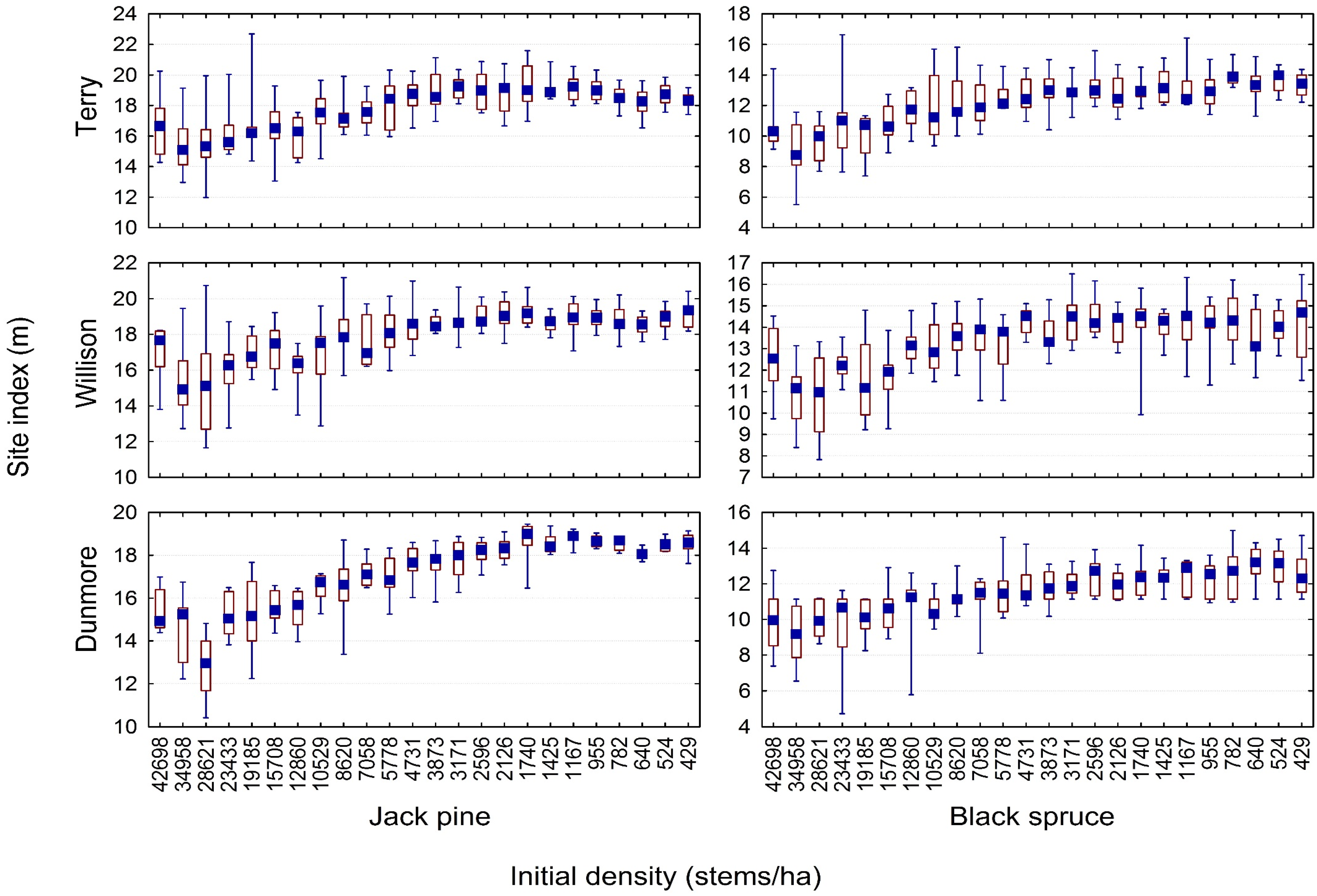
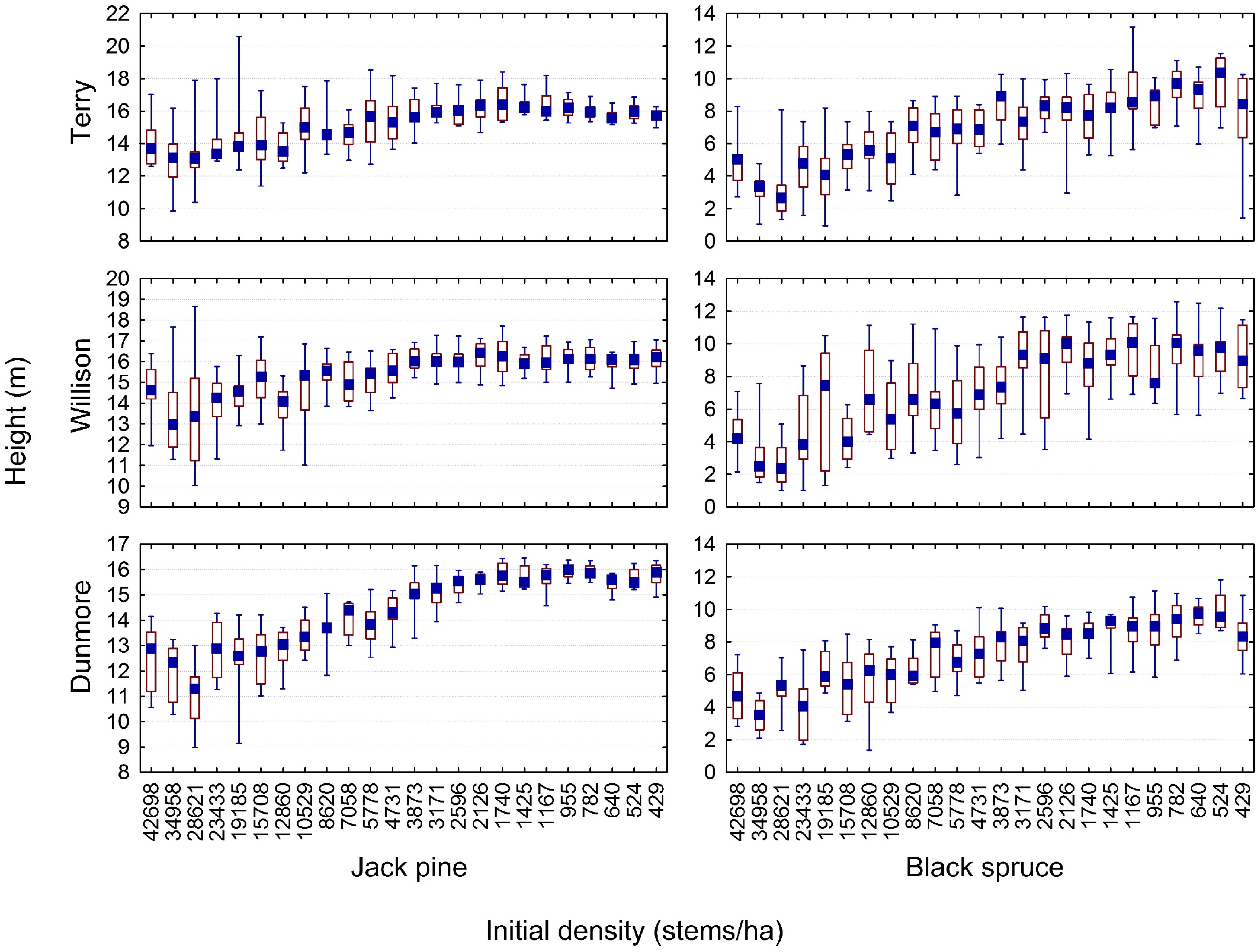
3.1. Experimental Evidence of a Density-Dependent Height Repression Effect

The density-dependent height repression effect on jack pine and black spruce at approximately 40 years post-establishment within the 3 Nelder plot clusters is shown in Figure 1: declining mean height with increasing density for trees on identical site qualities and of equal age. Note, due to potential edge effects, inferences were limited to the patterns shown between the nominal initial spacings of 28,621 stems/ha (3rd concentric arc) and 524 stems/ha (23rd concentric arc). Furthermore, using the mean height values of the tallest trees as a surrogate for mean dominant height, the resultant density-dependent height repression effect in terms of site index is illustrated in Figure 2. Site index was defined as the mean dominant height at a base-age of 50 years breast-height as determined from Ontario-based site index functions developed for jack pine and black spruce by Carmean ([23] and [24], respectively). These graphical trends indicated a reduction in productivity with increasing density for both species across all 3 clusters. The pattern of the reduction was nonlinear in nature: site index estimates increased, reaching a plateau and then slightly declined as density decreased. Note, for jack pine for which the data permitted, the repression effect intensified over time as indicated by a gradual shift in the asymptote (peak) towards the lower densities and by the increasing gradient (slope) of the height-density relationship with age (graphic not shown). Graphically assessing the height–density relationship pattern for jack pine at 16, 20 and 40 years post-establishment, and for black spruce at 41 years post-establishment, indicated a consistent pattern of declining productivity with increasing density between 1425 stems/ha and 28,621 stems/ha (e.g., Figure 1 and Figure 2). However, the rate of decline was species-specific and visually more evident for jack pine than for black spruce.

Figure 1. Box and whisker plots graphically illustrating the observed relationship between initial spacing and mean height at approximately 40 year post-establishment by species and plot series. Note, the median value is denoted by the solid square within the open rectangle, first and third quartiles are denoted by the lower and upper horizontal sides of the open rectangle, respectively, and minimum and maximum values are denoted by the end points of the lower and upper whiskers, respectively.

Figure 1. Box and whisker plots graphically illustrating the observed relationship between initial spacing and mean height at approximately 40 year post-establishment by species and plot series. Note, the median value is denoted by the solid square within the open rectangle, first and third quartiles are denoted by the lower and upper horizontal sides of the open rectangle, respectively, and minimum and maximum values are denoted by the end points of the lower and upper whiskers, respectively.

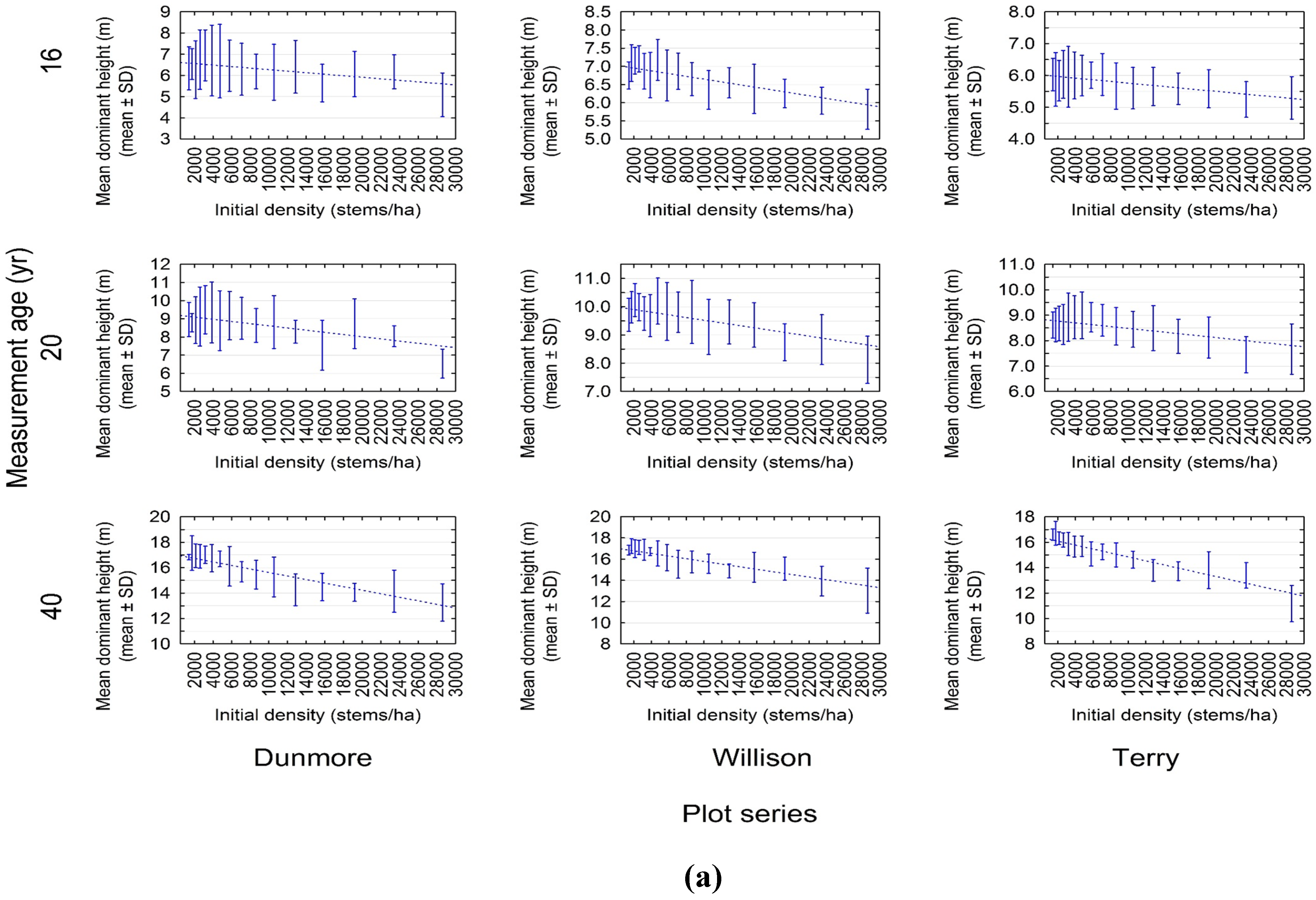
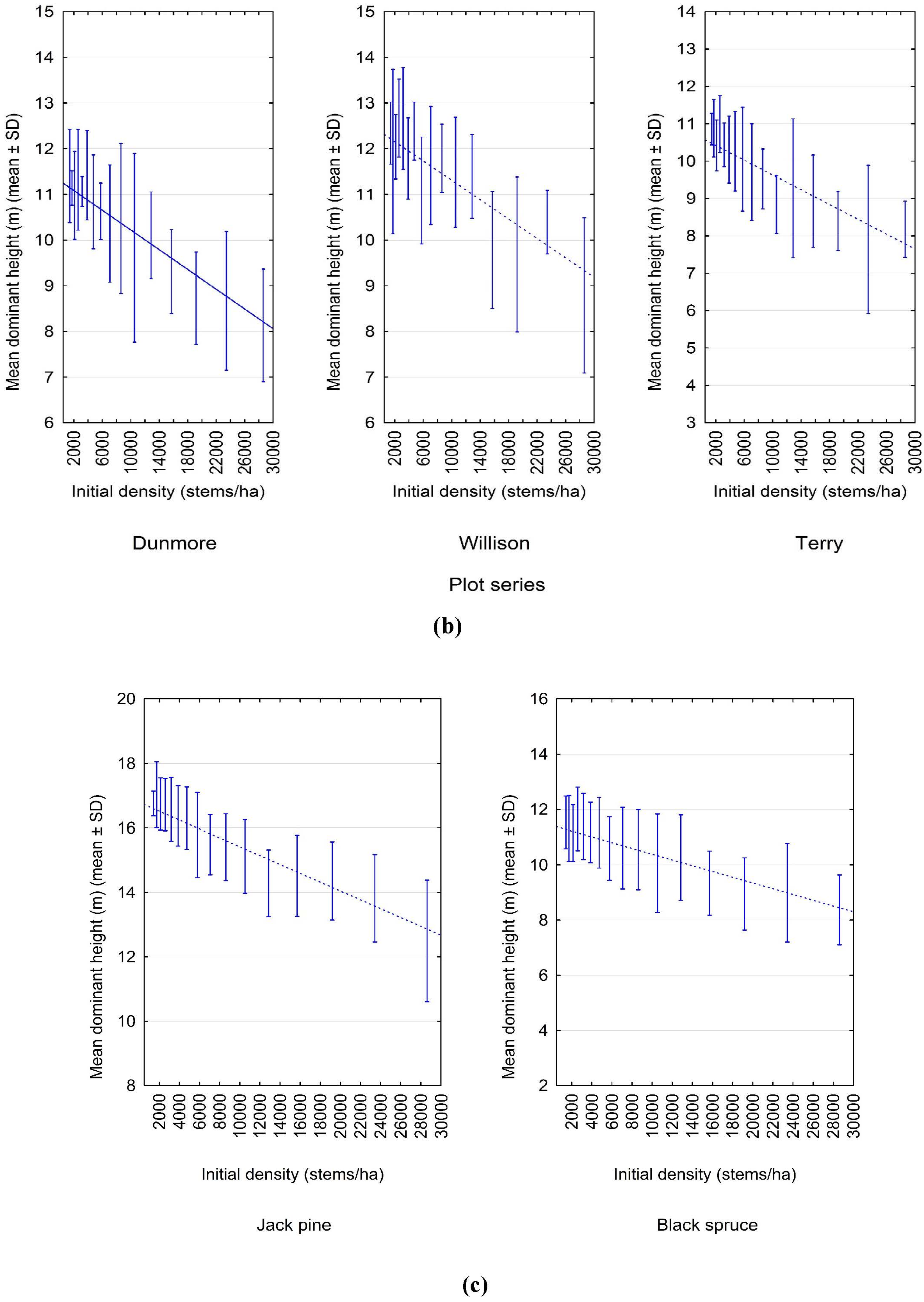
3.2. Quantifying the Density-Dependent Height Repression Effect

As presented in Table 1, the occurrence of spatial correlation based on time series statistics was quantified by the ratio of the number of plots exhibiting significant (p ≤ 0.05) partial autocorrelation coefficients to the total number of plots assessed by species, cluster and measurement time. Thus, based on the data from the initial spacing densities of 1425 stems/ha to 28.621 stems/ha, the frequency of spatial correlation as detected by the partial autocorrelation coefficient was relatively low. Specifically, the results indicated significant (p ≤ 0.05) spatial correlation only at the 1st spatial lag. Only 27% (n = 22) of all the jack pine relationships assessed and only 33% (n = 9) of all the black spruce relationships, exhibited spatial correlation effects (Table 1). For jack pine, the occurrence of significant (p ≤ 0.05) partial autocorrelation coefficients increased over time: 18%, 29% and 33% of the relationships at age 16, 20 and 40 years, respectively (Table 1). For both species, the partial autocorrelation coefficients were only significant (p ≤ 0.05) at the 1st spatial lag suggesting that when present, spatial correlation effects were operating only between first order neighbours (Table 1).

Figure 2. Box and whisker plots graphically illustrating the observed relationship between initial spacing and site productivity by species and plot series. Note, box and whisker plot denotations are given in Figure 1.

Figure 2. Box and whisker plots graphically illustrating the observed relationship between initial spacing and site productivity by species and plot series. Note, box and whisker plot denotations are given in Figure 1.

The results from the second part of the spatial autocorrelation detection procedure, which employed regression analysis to determine the significant association among residual errors, indicated that the density-dependent effects on height development were frequent: significant (p ≤ 0.05) linear relationships with negative slope estimates in 54 of the 83 jack pine relationships (65%), and in 24 of the 27 black spruce relationships (89%). In regards to jack pine, the occurrence of density-dependent height repression increased over time: significant (p ≤ 0.05) linear relationships with negative slope estimates detected in 50%, 57% and 89% of the relationships at ages 16, 20 and 40, respectively. As presented in Table 1, the occurrence of spatial correlation based on regression analysis was quantified by the ratio of the number of plots exhibiting significant (p ≤ 0.05) correlation among adjacent regression residuals (${\widehat{p}}_1$) to the total number of plots assessed by species, cluster and measurement time. Over all the clusters and measurement times, the results indicated that the frequency of significant residual regression relationships was low for jack pine (11%) and totally absence in regards to black spruce (Table 1). For the significant jack pine relationships, the magnitude of ${\widehat{p}}_1$ was considerably less than unity: mean (min/max) absolute ${\widehat{p}}_1$ of 0.571 (0.462/0.733). These results indicate that the evidence of significant spatial autocorrelation effects was infrequent for jack pine and completely lacking for black spruce.

Table 1. Plot-level detection of spatial autocorrelation by species and measurement age.

Species	Age	Nelder Plot Series	Spatial Autocorrelation Detection via Time Series Statistics a		Spatial Autocorrelation Detection via Regression Statistics b
			Frequency of significant partial autocorrelation coefficients (ns/nt)	Spatial lag	Frequency of significant density-dependent height repression effects (n’s/nt)	Frequency of significant spatial autocorrelation (n’’s/n’s)
Jack	16	Dunmore	1/10	1st	3/10	1/3
Pine		Willison	3/9	1st	6/9	0/6
		Terry	1/9	1st	5/9	0/5
	20	Dunmore	1/10	1st	3/10	1/3
		Willison	2/9	1st	7/9	0/7
		Terry	5/9	1st	6/9	1/6
	40	Dunmore	3/10	1st	8/10	0/8
		Willison	2/9	1st	8/9	2/8
		Terry	4/8	1st	8/8	1/8
Black	41	Dunmore	3/10	1st	8/10	0/8
Spruce		Willison	3/9	1st	8/9	0/8
		Terry	3/8	1st	8/8	0/8

^a Ratio of the number of significant (p ≤ 0.05) partial autocorrelation coefficients (n_s) to the total number of plots assessed (n_t) within a specified Nelder plots series at a specified measurement age; ^b (1) Ratio of the number of significant (p ≤ 0.05) mean dominant height—initial density regression relationships (n’_s) to the total number of plots assessed (n_t) within a specified Nelder plots series at a specified measurement age; and (2) Ratio of the number of significant (p ≤ 0.05) residual regressions (n’’_s) to the total number of significant relationships (n’_s) found in (1) for a given plot series and measurement age.

Table 1. Plot-level detection of spatial autocorrelation by species and measurement age.

Species	Age	Nelder Plot Series	Spatial Autocorrelation Detection via Time Series Statistics a		Spatial Autocorrelation Detection via Regression Statistics b
			Frequency of significant partial autocorrelation coefficients (ns/nt)	Spatial lag	Frequency of significant density-dependent height repression effects (n’s/nt)	Frequency of significant spatial autocorrelation (n’’s/n’s)
Jack	16	Dunmore	1/10	1st	3/10	1/3
Pine		Willison	3/9	1st	6/9	0/6
		Terry	1/9	1st	5/9	0/5
	20	Dunmore	1/10	1st	3/10	1/3
		Willison	2/9	1st	7/9	0/7
		Terry	5/9	1st	6/9	1/6
	40	Dunmore	3/10	1st	8/10	0/8
		Willison	2/9	1st	8/9	2/8
		Terry	4/8	1st	8/8	1/8
Black	41	Dunmore	3/10	1st	8/10	0/8
Spruce		Willison	3/9	1st	8/9	0/8
		Terry	3/8	1st	8/8	0/8

^a Ratio of the number of significant (p ≤ 0.05) partial autocorrelation coefficients (n_s) to the total number of plots assessed (n_t) within a specified Nelder plots series at a specified measurement age; ^b (1) Ratio of the number of significant (p ≤ 0.05) mean dominant height—initial density regression relationships (n’_s) to the total number of plots assessed (n_t) within a specified Nelder plots series at a specified measurement age; and (2) Ratio of the number of significant (p ≤ 0.05) residual regressions (n’’_s) to the total number of significant relationships (n’_s) found in (1) for a given plot series and measurement age.

Therefore, based on the results of these spatial correlation detection analyses which indicated that low levels of spatial autocorrelation were present in only a minority of the plots irrespective of species, it was concluded that there was insufficient evidence to negate the use the OLS parameterization methods in quantifying the height-density relationships. Thus assuming that spatial correlation effects were minimal and inconsequential, a common OLS regression analytical framework was used to estimate the density-dependent height repression parameter: ${\text{β}}_1$ from the $H_d={\widehat{\beta }}_0+{\widehat{\beta }}_1{N}_e$ relationship.

For each of the resultant significant relationships, the presence of potential outliers and influential observations were determined via the use of predictor variable—raw residual graphs in association with residual statistics (i.e., studentized deleted residuals and Cook’s distance measures, respectively, where the probability level for exclusion was set at 0.01 for both measures [25]). Although no influential observations were detected, outliers were present in 19 of the relationships. These outliers were removed and the models reparameterized and reassessed for compliance with regression assumptions, including the reassessment of the presence of spatial autocorrelation effects.

Table A1. Plot-level species-specific parameter estimates and associated regression statistics for significant (p ≤ 0.05) mean dominant height-density relationships by measurement age.

Species	Age	Nelder Plot Series	Plot No.	Parameter Estimates a					Regression Statistics b
				Intercept		Slope (height-repression coefficient)			DF	r2	SEE (m)	F-ratio
				Estimate	SE	Estimate	95% CL		nreg, nres
							Lower	Upper
Jack Pine	16	Dunmore	1	7.20	0.143	−0.0000450	−0.0000696	−0.0000205	1,14	0.525	0.371	15.5 *
			5	7.65	0.175	−0.0000554	−0.0000856	−0.0000253	1,14	0.526	0.455	15.5 *
			9	5.25	0.150	−0.0000281	−0.0000539	−0.0000022	1,14	0.279	0.390	5.4 *
		Willison	11	7.83	0.115	−0.0000612	−0.0000809	−0.0000415	1,14	0.760	0.298	44.2 *
			12	6.91	0.114	−0.0000260	−0.0000459	−0.0000061	1,13	0.381	0.296	8.0 *
			13	7.32	0.134	−0.0000378	−0.0000607	−0.0000149	1,13	0.495	0.342	12.8 *
			14	6.97	0.164	−0.0000593	−0.0000876	−0.0000310	1,14	0.590	0.427	20.2 *
			16	6.60	0.131	−0.0000433	−0.0000659	−0.0000207	1,14	0.547	0.341	16.9 *
			17	6.99	0.125	−0.0000450	−0.0000666	−0.0000234	1,14	0.588	0.326	20.0 *
		Terry	22	7.18	0.112	−0.0000399	−0.0000593	−0.0000205	1,14	0.582	0.292	19.5 *
			23	5.88	0.108	−0.0000265	−0.0000451	−0.0000079	1,14	0.401	0.280	9.4 *
			25	5.55	0.092	−0.0000205	−0.0000363	−0.0000046	1,14	0.354	0.239	7.7 *
			26	5.56	0.073	−0.0000314	−0.0000440	−0.0000188	1,14	0.671	0.190	28.5 *
			28	6.05	0.093	−0.0000250	−0.0000407	−0.0000093	1,13	0.476	0.232	11.8 *
	20	Dunmore	1	9.64	0.209	−0.0000604	−0.0000965	−0.0000243	1,14	0.479	0.544	12.9 *
			5	10.53	0.283	−0.0001142	−0.0001629	−0.0000654	1,14	0.643	0.736	25.2 *
			9	7.88	0.193	−0.0000495	−0.0000827	−0.0000162	1,14	0.421	0.501	10.2 *
		Willison	11	10.99	0.188	−0.0000848	−0.0001171	−0.0000525	1,14	0.693	0.488	31.7 *
			12	9.87	0.129	−0.0000287	−0.0000512	−0.0000062	1,13	0.369	0.335	7.6 *
			13	10.29	0.161	−0.0000435	−0.0000709	−0.0000161	1,13	0.475	0.410	11.8 *
			14	10.11	0.181	−0.0000930	−0.0001241	−0.0000619	1,14	0.746	0.469	41.1 *
			15	10.87	0.241	−0.0000655	−0.0001070	−0.0000240	1,14	0.450	0.626	11.5 *
			16	9.06	0.152	−0.0000611	−0.0000873	−0.0000349	1,14	0.640	0.396	24.9 *
			17	9.90	0.160	−0.0000694	−0.0000969	−0.0000418	1,14	0.676	0.416	29.2 *
		Terry	22	10.33	0.214	−0.0000606	−0.0000975	−0.0000237	1,14	0.470	0.557	12.4 *
			23	8.78	0.125	−0.0000367	−0.0000582	−0.0000151	1,14	0.487	0.325	13.3 *
			25	8.46	0.084	−0.0000610	−0.0000755	−0.0000466	1,14	0.854	0.218	82.0 *
			26	8.52	0.126	−0.0000579	−0.0000796	−0.0000362	1,14	0.700	0.327	32.7 *
			28	8.92	0.120	−0.0000227	−0.0000430	−0.0000025	1,13	0.312	0.298	5.9 *
			29	8.72	0.146	−0.0000481	−0.0000732	−0.0000230	1,14	0.547	0.378	16.9 *
	40	Dunmore	1	17.55	0.392	−0.0001911	−0.0002585	−0.0001236	1,14	0.725	1.018	36.9 *
			2	16.68	0.321	−0.0001829	−0.0002396	−0.0001261	1,13	0.788	0.833	48.5 *
			3	17.16	0.337	−0.0001396	−0.0001992	−0.0000799	1,13	0.663	0.875	25.6 *
			4	18.31	0.471	−0.0001326	−0.0002184	−0.0000469	1,13	0.462	1.221	11.2 *
			6	17.63	0.288	−0.0001510	−0.0002006	−0.0001013	1,14	0.753	0.748	42.6 *
			7	16.51	0.230	−0.0001383	−0.0001779	−0.0000988	1,14	0.801	0.597	56.2 *
			8	16.26	0.406	−0.0001199	−0.0001897	−0.0000500	1,14	0.492	1.054	13.5 *
			10	16.59	0.489	−0.0001166	−0.0002008	−0.0000324	1,14	0.387	1.270	8.8 *
		Willison	11	18.16	0.353	−0.0001393	−0.0002002	−0.0000785	1,14	0.633	0.918	24.1 *
			12	17.41	0.288	−0.0000896	−0.0001397	−0.0000395	1,13	0.535	0.746	14.9 *
			13	17.64	0.235	−0.0001261	−0.0001661	−0.0000861	1,13	0.781	0.599	46.4 *
			14	16.84	0.381	−0.0001350	−0.0002007	−0.0000694	1,14	0.582	0.990	19.5 *
			16	16.58	0.286	−0.0001943	−0.0002435	−0.0001451	1,13	0.848	0.737	72.7 *
			17	16.84	0.293	−0.0001993	−0.0002551	−0.0001434	1,13	0.821	0.749	59.4 *
			18	16.63	0.333	−0.0001078	−0.0001657	−0.0000499	1,13	0.554	0.863	16.1 *
			19	17.25	0.376	−0.0001349	−0.0001996	−0.0000702	1,13	0.610	0.968	20.3 *
		Terry	23	17.11	0.448	−0.0001933	−0.0002705	−0.0001160	1,14	0.673	1.165	28.8 *
			24	15.94	0.438	−0.0001668	−0.0002422	−0.0000914	1,14	0.616	1.138	22.5 *
			25	16.48	0.267	−0.0002068	−0.0002527	−0.0001608	1,14	0.869	0.693	93.1 *
			26	16.46	0.229	−0.0001492	−0.0001908	−0.0001075	1,13	0.821	0.593	59.8 *
			27	16.54	0.168	−0.0001339	−0.0001630	−0.0001047	1,13	0.883	0.434	98.4 *
			28	17.10	0.264	−0.0002240	−0.0002694	−0.0001785	1,14	0.889	0.685	111.8 *
			29	16.19	0.388	−0.0001184	−0.0001872	−0.0000496	1,13	0.515	1.009	13.8 *
			30	16.36	0.347	−0.0001500	−0.0002092	−0.0000909	1,13	0.698	0.886	30.0 *
Black Spruce	41	Dunmore	1	11.33	0.210	−0.0001484	−0.0001867	−0.0001101	1,13	0.844	0.545	70.2 *
			2	10.84	0.142	−0.0000723	−0.0000968	−0.0000479	1,14	0.742	0.369	40.2 *
			4	13.04	0.433	−0.0001076	−0.0001821	−0.0000331	1,14	0.407	1.124	9.6 *
			6	12.11	0.311	−0.0001176	−0.0001712	−0.0000640	1,14	0.613	0.809	22.1 *
			7	11.13	0.338	−0.0001390	−0.0001972	−0.0000808	1,14	0.652	0.878	26.2 *
			8	10.90	0.256	−0.0001135	−0.0001576	−0.0000695	1,14	0.686	0.665	30.5 *
			9	10.95	0.370	−0.0001124	−0.0001761	−0.0000487	1,14	0.506	0.961	14.3 *
			10	11.26	0.253	−0.0001806	−0.0002243	−0.0001370	1,14	0.849	0.658	78.9 *
		Willison	11	13.09	0.435	−0.0001188	−0.0001938	−0.0000438	1,14	0.452	1.131	11.6 *
			12	12.67	0.375	−0.0001805	−0.0002451	−0.0001159	1,14	0.720	0.975	35.9 *
			14	11.33	0.465	−0.0001129	−0.0001930	−0.0000328	1,14	0.395	1.209	9.1 *
			15	13.04	0.178	−0.0000712	−0.0001019	−0.0000405	1,14	0.639	0.463	24.7 *
			16	12.95	0.179	−0.0001717	−0.0002023	−0.0001412	1,13	0.919	0.457	147.8 *
			17	11.37	0.407	−0.0000943	−0.0001644	−0.0000243	1,14	0.373	1.057	8.3 *
			18	12.97	0.290	−0.0001332	−0.0001831	−0.0000833	1,14	0.701	0.753	32.8 *
			19	12.92	0.473	−0.0001140	−0.0001954	−0.0000325	1,14	0.391	1.229	9.0 *
		Terry	23	10.61	0.290	−0.0000926	−0.0001425	−0.0000427	1,14	0.531	0.752	15.9 *
			24	10.78	0.293	−0.0001468	−0.0001973	−0.0000963	1,14	0.735	0.762	38.8 *
			25	10.23	0.538	−0.0001838	−0.0002765	−0.0000911	1,14	0.564	1.399	18.1 *
			26	10.72	0.222	−0.0001025	−0.0001402	−0.0000648	1,13	0.726	0.563	34.5 *
			27	10.19	0.261	−0.0001130	−0.0001578	−0.0000681	1,14	0.676	0.677	29.2 *
			28	11.05	0.303	−0.0000735	−0.0001258	−0.0000213	1,14	0.394	0.789	9.1 *
			29	11.33	0.355	−0.0000989	−0.0001601	−0.0000378	1,14	0.462	0.923	12.0 *
			30	11.17	0.339	−0.0000947	−0.0001532	−0.0000363	1,14	0.463	0.882	12.1 *

^a OLS parameter estimates for the intercept $({\beta }_0)$ with associated standard error (SE), and slope $({\beta }_1)$ with associated lower and upper 95% confidence limits (95% CL). ^b Degrees of freedom (DF) for regression and residual error (n_reg and n_res, respectively), coefficient of determination (r²), standard error of the estimate (SEE), and F-statistic (F-ratio). Note, F-ratios superscripted by * denotes a significant (p ≤ 0.05) relationship.

provides the parameter estimates and associated regression statistics for the resultant 54 jack pine and 24 black spruce significant (p ≤ 0.05) relationships. The associated residual analyses indicated that the models satisfactorily described the H_d-N_e relationships. The regression equations explained a moderate level of variation: mean (minimum/maximum) coefficient of determination (r²) values of 0.512 (0.279/0.760), 0.560 (0.312/0.854), 0.683 (0.387/0.889) for jack pine at ages 16, 20 and 40, respectively, and 0.602 (0.373/0.919) for black spruce at age 41. The magnitude of error was acceptable as reflected by moderate levels of the standard error of the estimate: mean (minimum/maximum) of 0.320 m (0.190/0.455), 0.439 m (0.218/0.736), 0.866 m (0.434/1.270) for jack pine at age 16, 20 and 40, respectively, and 0.834 m (0.369/1.399) for black spruce at age 41. Overall, the regression relationships were in general compliance with the constant variance and normality assumptions underlying OLS parameterization (e.g., horizontal band and invariant pattern of raw residuals when plotted against the predictor variable).

The frequency and magnitude of the density-dependent height repression effect increased over time as evident by the temporal increase in the number of significant relationships for jack pine (14, 16 and 24 at 16, 20 and 40 years post-establishment, respectively) and increasing negativity of slope estimates: mean (minimum/maximum) slope values of −0.000039 (−0.000061/−0.000021), −0.000060 (−0.000114/0.000023) and −0.000152 (−0.000224/−0.000224) at 16, 20 and 40 years post-establishment, respectively (Table A1). For jack pine, where multiple temporal relationships were available, the height repression effect was linear in nature and intensified over time as inferred from the temporal increase in the negativity of the slope values (Figure 3a; Table 2). In fact, the intensity of the repression effect as measured by the magnitude of the slope parameter estimate increased almost 5 fold from age 16 to age 40: the mean slope was −0.00003 at age 16 versus its value of −0.00014 at age 40. Figure 3b presents the height–density relationship for black spruce for the remeasurements taken at age 41 for each of the 3 Nelder plot clusters whereas Figure 3c illustrates the pooled relationship for each species, approximately 40 years after establishment.

Figure 3. Bivariate scatter plots illustrating the relationship between initial density and mean height for (a) jack pine at approximately 16, 20 and 40 years post-establishment for each Nelder plot series; (b) black spruce at approximately 40 years post-establishment for each Nelder plot series; and (c) jack pine and black spruce at approximately 40 years post-establishment for all the Nelder plots combined. The whiskers defined the mean ± standard deviation (SD) values and the dotted line is the estimated height-density relationship for the height repression coefficients given in Table 2.

Figure 3. Bivariate scatter plots illustrating the relationship between initial density and mean height for (a) jack pine at approximately 16, 20 and 40 years post-establishment for each Nelder plot series; (b) black spruce at approximately 40 years post-establishment for each Nelder plot series; and (c) jack pine and black spruce at approximately 40 years post-establishment for all the Nelder plots combined. The whiskers defined the mean ± standard deviation (SD) values and the dotted line is the estimated height-density relationship for the height repression coefficients given in Table 2.

Table 2. Resultant mean dominant height-density relationship by species, age and plot series inclusive of the density-dependent height repression coefficient estimates and their 95% confidence limits.

Species	Age	Plot Series	n	Intercept	Density-Dependent Height Repression Coefficient a
					95% CI-L	${\widehat{\beta }}_1^{*}$	95% CI-U
Jack Pine	16	Dunmore	3	6.634	−0.000130	−0.000036	0.000058
		Willison	6	7.028	−0.000080	−0.000038	0.000004
		Terry	5	6.019	−0.000059	−0.000026	0.000007
		Combined	14	6.563	−0.000050	−0.000031	−0.000012
	20	Dunmore	3	9.215	−0.000216	−0.000060	0.000096
		Willison	7	9.993	−0.000094	−0.000047	0.000000
		Terry	6	8.840	−0.000077	−0.000036	0.000005
		Combined	16	9.384	−0.000067	−0.000042	−0.000018
	40	Dunmore	8	17.007	−0.000256	−0.000139	−0.000021
		Willison	8	17.032	−0.000232	−0.000124	−0.000017
		Terry	8	16.385	−0.000286	−0.000154	−0.000023
		Combined	24	16.789	−0.000200	−0.000137	−0.000078
Black Spruce	41	Dunmore	8	11.300	−0.000202	−0.000108	−0.000015
		Willison	8	12.367	−0.000198	−0.000106	−0.000014
		Terry	8	10.624	−0.000185	−0.000099	−0.000014
		Combined	24	11.429	−0.000150	−0.000104	−0.000059

^a Grand mean density-dependent height repression coefficient as calculated by Equation (1) and associated lower and upper 95% confidence limits (denoted CI-L and CI-U, respectively).

Table 2. Resultant mean dominant height-density relationship by species, age and plot series inclusive of the density-dependent height repression coefficient estimates and their 95% confidence limits.

Species	Age	Plot Series	n	Intercept	Density-Dependent Height Repression Coefficient a
					95% CI-L	${\widehat{\beta }}_1^{*}$	95% CI-U
Jack Pine	16	Dunmore	3	6.634	−0.000130	−0.000036	0.000058
		Willison	6	7.028	−0.000080	−0.000038	0.000004
		Terry	5	6.019	−0.000059	−0.000026	0.000007
		Combined	14	6.563	−0.000050	−0.000031	−0.000012
	20	Dunmore	3	9.215	−0.000216	−0.000060	0.000096
		Willison	7	9.993	−0.000094	−0.000047	0.000000
		Terry	6	8.840	−0.000077	−0.000036	0.000005
		Combined	16	9.384	−0.000067	−0.000042	−0.000018
	40	Dunmore	8	17.007	−0.000256	−0.000139	−0.000021
		Willison	8	17.032	−0.000232	−0.000124	−0.000017
		Terry	8	16.385	−0.000286	−0.000154	−0.000023
		Combined	24	16.789	−0.000200	−0.000137	−0.000078
Black Spruce	41	Dunmore	8	11.300	−0.000202	−0.000108	−0.000015
		Willison	8	12.367	−0.000198	−0.000106	−0.000014
		Terry	8	10.624	−0.000185	−0.000099	−0.000014
		Combined	24	11.429	−0.000150	−0.000104	−0.000059

^a Grand mean density-dependent height repression coefficient as calculated by Equation (1) and associated lower and upper 95% confidence limits (denoted CI-L and CI-U, respectively).

4. Discussion

The results of this study indicated that the height repression effect, as quantified by the slope of the hight-density relationship, was greater for jack pine than for black spruce on both a cluster and collective basis (e.g., approximately 25% greater overall at approximately 40 years post-establishment (Table 2)). Given that (1) site occupancy as measured by relative density index was within the conceptual zone of imminent competition-mortality in which self-thinning is expected to occur (e.g., compare the mean relative densities of 1.08 and 0.62 for jack pine and black spruce across the 3rd to the 18th concentric arcs, respectively, against the 0.50 value at which full occupancy is achieved [26]); and (2) observational evidence from the last remeasurements indicated the occurrence of ongoing self-thinning, the plots were considered to be exceeding their conceptual full occupancy levels. Consequently, density-dependent effects were considered to be fully expressed and thus future temporal increases in density repression effects were assumed to be negligible. Therefore based on supporting research findings in which height growth was found to be density-dependent for some conifers [10,11,12,13,14,15] and the empirically-evident density-dependence height repression exhibited by jack pine and black spruce within the studied Nelder plots (Figure 1, Figure 2 and Figure 3), the existence of a density-dependent height repression effect for these species is acknowledged.

The empirical evidence provided by these initial spacing experiments supported the inference that density-dependent height repression effects exist for jack pine and black spruce when grown at high density-stress levels. Given the importance of such a finding, in terms of the consequences for modelling responses to density manipulation treatments and the broader implications for forest estate modeling, further investigation is warranted. The pattern of the repression effect observed from the initial spacing experiments (Figure 1 and Figure 2) was nonlinear in nature: productivity increased with declining density until reaching a plateau and thereafter stabilized or slightly declined. From a biological perspective, this latter declining phase was particularly evident for jack pine at initial establishment densities of less than 800 stems/ha. This may be due to a relaxation of this species strong epinastic control resulting in an increased allocation of photosynthetic resources to the production of branch and crown components at the expense of height growth.

Compared to other boreal conifers species such as lodgepole pine, the observed repression effect for jack pine and black spruce was similar in terms of magnitude. Model-based results presented by Cieszewski and Bella [14] suggest that the height repression effect at an index age of 50 years (breast-height age) between lodgepole pine stands with densities of 2000 and 40,000 stems/ha, was approximately 35% (derived through graphical interpolation of Figure 2 in Cieszewski and Bella [14] for poor medium and good site qualities). Based on the extrapolation of the pooled equations presented in Table 2 and shown in Figure 3c, comparison of height differences at an approximate age of 40 years post-establishment between jack pine and black spruce stands established at densities of 2000 and 40,000 stems/ha, indicated relative height repression effects of 32% and 37%, respectively. In the case of a more realistic range of densities at which forest management typically operates (2000–10,000 stems/ha), the height repression effect is substantially reduced: 7% and 10% for jack pine and black spruce, respectively. Analytical solutions for accounting for repression effects when developing site index equations and their height-age analogues could include the calibration of separate functions for different management intensities (e.g., different functions for natural-orgin stands and plantations), employing empirical-based corrective adjustments within the model specifications (e.g., [27]), or developing entirely new models in which stand density is explicitly included as a dynamic-based independent variable (sensu [14]).

The site-specific and assumed density-independent relationship between the stand height and age is central to the phytocentric approach used to estimate the productivity of even-aged monospecific boreal stand-types (e.g., site index as defined as the mean dominant height or top height at a specified index or base age [23,24,28]). Stand height is traditionally defined as the mean height of the dominant trees within a stand (e.g., mean height of the tallest trees within the upper quintile of the height distribution and traditionally denoted mean dominant height) or as the mean height of the trees with the largest diameters in a stand (e.g., mean height of the trees within the upper quintile of the diameter distribution which is traditionally denoted top height). Practically, mean dominant height and top height are mathematically similar given that the selection of the tallest trees implicitly corresponds to the selection of the largest diameter trees given the allometric scaling relationship between height and diameter for excurrent forest tree species: $d\propto h^{\beta }$ where β ranges from 1.0 (geometric similarity model) to 1.5 (elastic similarity model) [29]. Although in this study where the mean height of the tallest trees at each initial spacing was assumed to be measure of central tendency, it is not statistically equivalent to either dominant or top height given the limited number of observations available for calculating the mean height on the studied Nelder plots (e.g., n = 12). Analysis of larger and more geographically representative data sets derived from long-term density control experiments employing more traditional experimental designs (e.g., spatially replicated randomized complete block designs), would be of value in terms of informing and complementing the results obtained in this study.

Historically, the assumption that stand height could be used as an indirect indicator of stand productivity was originally derived from the observation that total stand volume for a given mean stand height remained constant across a range of site classes (i.e., Eichhorn’s rule sensu [9,30]). Site-specific relationships between stand height and age have also been used to quantify temporal change within numerous growth and yield models including empirical benchmark yield models [31] and density management decision-support models (e.g., structural stand density management models [6,7]). The assumption underlying the use of the stand height-age relationship for estimating site productivity and modeling stand dynamics is that height development is largely unaffected by stand density (sensu [32]). Stands grown within a nominal range of densities usually adhere to this assumption and evidence to the contrary has rarely been reported in the literature. However, this assumption has been shown to be untenable for some species when grown at very low densities where photosynthate is commonly redirected towards the production of crown structures (branches) at the expense of stem growth. Conversely, density-dependent repression in which dominant height development has been negatively influenced by increasing levels of density-stress have been reported for a number of even-aged monospecific coniferous stand-types (e.g., ponderosa pine (Pinus ponderosa L.; [10]), Douglas-fir (Pseudotsuga menziesii (Mirb.) Franco var. menziesii; [11]), loblolly pine (Pinus taeda L.; [12,13]), and lodgepole pine (Pinus contorta Dougl. ex Loud.; [14,15]).

Operationally, the acknowledgement that height growth may be negatively affected by density-stress may have important forest management implications. Particularly, given the reduction in establishment densities arising from wide spread use of plantation forestry throughout the Canadian Boreal Forest Region. These plantations are commonly established at considerably lower densities (e.g., 2000 stems/ha) than stands which have regenerated naturally following a stand replacing disturbance such as wildfire (e.g., 10,000 stems/ha). Consequently, the reverse effect of increasing height growth with decreasing stand density could result in increased volumetric productivity at the stand level and corresponding increases in annual cut allocations at the forest level (e.g., [33]). Further research involving meta-analytical reviews of long-term and geographically diverse initial spacing and thinning experiments could provide the necessary conformation evidence for such a consequential inference.

5. Conclusions

Density-dependent height repression effects were detected within jack pine and black spruce populations that were at asymptotic levels of site occupancy. Although the range of densities analyzed differ from those within stands established and managed in operational forest management, the inversely proportional stand height–density relationship offers modeling opportunities in terms of site productivity estimation. Furthermore, using these results to inform model specification for quantifying responses to various density management treatments, could increase the predictive precision of density management models resulting in improved decision-making [30,34].

References

1. Rowe, J.S. Forest Regions of Canada; Publication No. 1300; Government of Canada, Department of Environment, Canadian Forestry Service: Ottawa, ON, Canada, 1972.
2. OMNR (Ontario Ministry of Natural Resources). State of Ontario’s Forests; Queens Printer for Ontario: Toronto, ON, Canada, 2012; p. 73. [Google Scholar]
3. OMNRF (Ontario Ministry of Natural Resources and Forestry). Forest Management Guide to Silviculture in the Great Lakes-St. Lawrence and Boreal Forests of Ontario; Queens Printer for Ontario: Toronto, ON, Canada, 2015; p. 394. [Google Scholar]
4. McKinnon, L.M.; Kayahara, G.J.; White, R.G. Biological Framework for Commercial Thinning Even-aged Single-Species Stands of Jack Pine, White Spruce, and Black Spruce in Ontario. 2006. Available online: http://www.forestresearch.ca/images/stories/pdf/tr-046.pdf (accessed on 8 July 2015).
5. Bell, W.F.; Parton, J.; Joyce, D.; Reid, D.; Wester, M.; Stinson, A.; Kayahara, G.; Towill, B. Developing a silvicultural framework and definitions for use in forest management planning and practice. For. Chron. 2008, 84, 678–692. [Google Scholar] [CrossRef]
6. Newton, P.F. Development of an integrated decision-support model for density management within jack pine stand-types. Ecol. Model. 2009, 220, 3301–3324. [Google Scholar] [CrossRef]
7. Newton, P.F. A decision-support system for density management within upland black spruce stand-types. Environ. Model. Softw. 2012, 35, 171–187. [Google Scholar] [CrossRef]
8. Lanner, R.M. On the insensitivity of height growth to spacing. For. Ecol. Manag. 1985, 13, 143–148. [Google Scholar] [CrossRef]
9. Bontemps, J.D.; Bouriaud, O. Predictive approaches to forest site productivity: Recent trends, challenges and future perspectives. Forestry 2014, 87, 109–128. [Google Scholar] [CrossRef]
10. Lynch, D.W. Effects of Stocking on Site Measurement and Yield of Second-Growth Ponderosa Pine in the Inland Empire; USDA Forest Service Research Paper No. 56; USDA Forest Service Research: Washington, DC, USA, 1958.
11. Knowe, S.A. Effect of competition control treatments on height-age and height-diameter relationships in young Douglas-fir plantations. For. Ecol. Manag. 1994, 67, 101–111. [Google Scholar] [CrossRef]
12. MacFarlane, D.W.; Green, E.J.; Burkhart, H.E. Population density influences assessment and application of site index. Can. J. For. Res. 2000, 30, 1472–1475. [Google Scholar] [CrossRef]
13. Sharma, M.; Burkhart, H.E.; Amateis, R.L. Modeling the effect of density on the growth of Loblolly Pine trees. South. J. Appl. For. 2002, 26, 124–133. [Google Scholar]
14. Cieszewski, C.J.; Bella, I.E. Modeling density-related lodgepole pine height growth, using Czarnowski’s stand dynamics theory. Can. J. For. Res. 1993, 23, 2499–2506. [Google Scholar] [CrossRef]
15. Farnden, C.; Herring, L. Severely repressed lodgepole pine responds to thinning and fertilization: 19-year results. For. Chron. 2002, 78, 404–414. [Google Scholar] [CrossRef]
16. Nelder, J.A. New kinds of systematic designs for spacing experiments. Biometrics 1962, 18, 283–307. [Google Scholar] [CrossRef]
17. García, O. Estimating top height with variable plot sizes. Can. J. For. Res. 1998, 28, 1509–1517. [Google Scholar] [CrossRef]
18. Magnussen, S. Effect of plot size on estimates of top height in Douglas-fir. West. J. Appl. For. 1999, 14, 17–27. [Google Scholar]
19. Affleck, D.L.R. A Comparative Study of Spatial Analysis Methods for Forestry Nelder Experiments. Master’s Thesis, University of British Columbia, Vancouver, BC, Canada, 2001. [Google Scholar]
20. Gujarati, D.N. Essential of Econometrics, 3rd ed.; McGraw-Hill/Irwin Inc.: New York, NY, USA, 2006; p. 838. [Google Scholar]
21. Hedges, L.V.; Olkin, I. Statistical Methods for Meta-Analysis; Academic Press: New York, NY, USA, 1985; p. 369. [Google Scholar]
22. Becker, B.J.; Wu, M.J. The synthesis of regression slopes in meta-analysis. Stat. Sci. 2007, 22, 414–429. [Google Scholar] [CrossRef]
23. Carmean, W.H.; Niznowski, G.P.; Hazenberg, G. Polymorphic site index curves for jack pine in Nothern Ontario. For. Chron. 2001, 77, 141–150. [Google Scholar] [CrossRef]
24. Carmean, W.H.; Hazenberg, G.; Deschamps, K.C. Polymorphic site index curves for black spruce and trembling aspen in northwest Ontario. For. Chron. 2006, 82, 231–242. [Google Scholar] [CrossRef]
25. Neter, J.; Wasserman, W.; Kutner, M.H. Applied Linear Statistical Models, 3rd ed.; Irwin: Boston, MA, USA, 1990; p. 878. [Google Scholar]
26. Newton, P.F. Forest production model for upland black spruce stands—Optimal site occupancy levels for maximizing net production. Ecol. Model. 2006, 190, 190–204. [Google Scholar] [CrossRef]
27. Alexander, R.R.; Tackle, D.; Dahms, W.G. Site Indexes for Lodgepole Pine with Corrections for Stand Density: Methodology; USDA, Forest Service Research Paper RM-29; USDA Forest Service Research: Washington, DC, USA, 1967.
28. Sharma, M.; Subedi, N.; Ter-Mikaelian, M.; Parton, J. Modeling climatic effects on stand height/site index of plantation grown jack pine and black spruce trees. For. Sci. 2015, 61, 25–34. [Google Scholar]
29. Niklas, K.J. Plant Allometry: Scaling of Form and Process; University of Chicago Press: Chicago, IL, USA, 1994; p. 395. [Google Scholar]
30. Newton, P.F. Evaluating the ecological integrity of structural stand density management models developed for boreal conifers. Forests 2015, 6, 992–1030. [Google Scholar] [CrossRef]
31. Penner, M.; Woods, M.; Parton, J.; Stinson, A. Validation of empirical yield curves for natural-origin stands in boreal Ontario. For. Chron. 2008, 84, 704–717. [Google Scholar] [CrossRef]
32. Weiskittel, A.R.; Hann, D.W.; Kershaw, J.A.; Vanclay, J.K. Forest Growth and Yield Modeling; John Wiley and Sons: West Sussex, UK, 2011; p. 415. [Google Scholar]
33. Huang, S.; Monserud, R.A.; Braun, T.; Lougheed, H.; Bakowsky, O. Comparing site productivity of mature fire-origin and post-harvest juvenile lodgepole pine stands in Alberta. Can. J. For. Res. 2004, 34, 1181–1191. [Google Scholar] [CrossRef]
34. Newton, P.F. Quantifying growth responses of black spruce and jack pine to thinning within the context of density management decision-support systems. Open J. For. 2015, 5, 409–421. [Google Scholar] [CrossRef]