
Detecting Stems in Dense and Homogeneous Forest Using Single-Scan TLS


Abstract
:1. Introduction
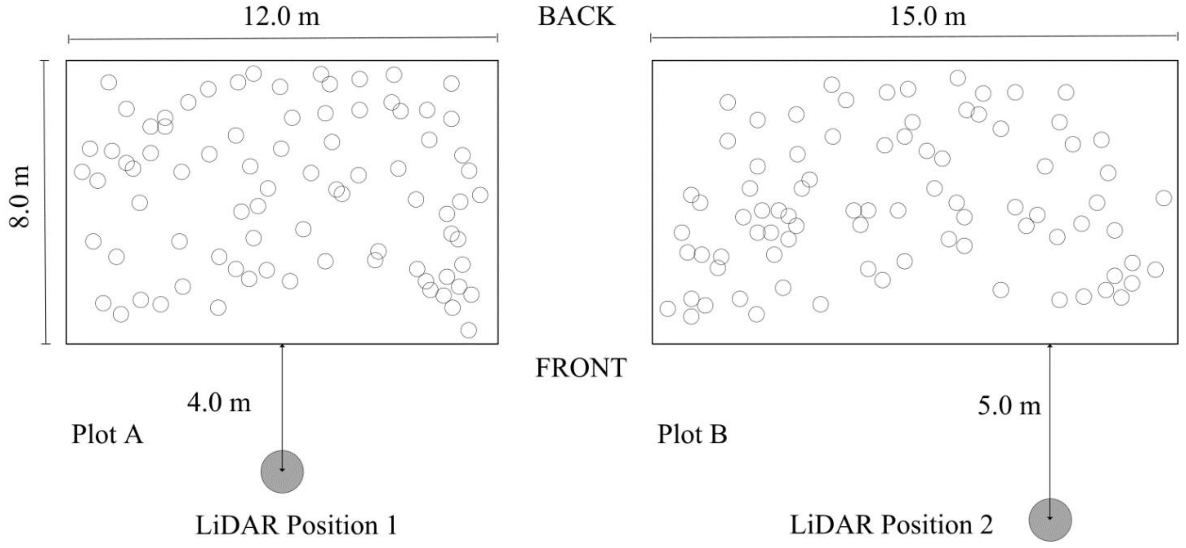
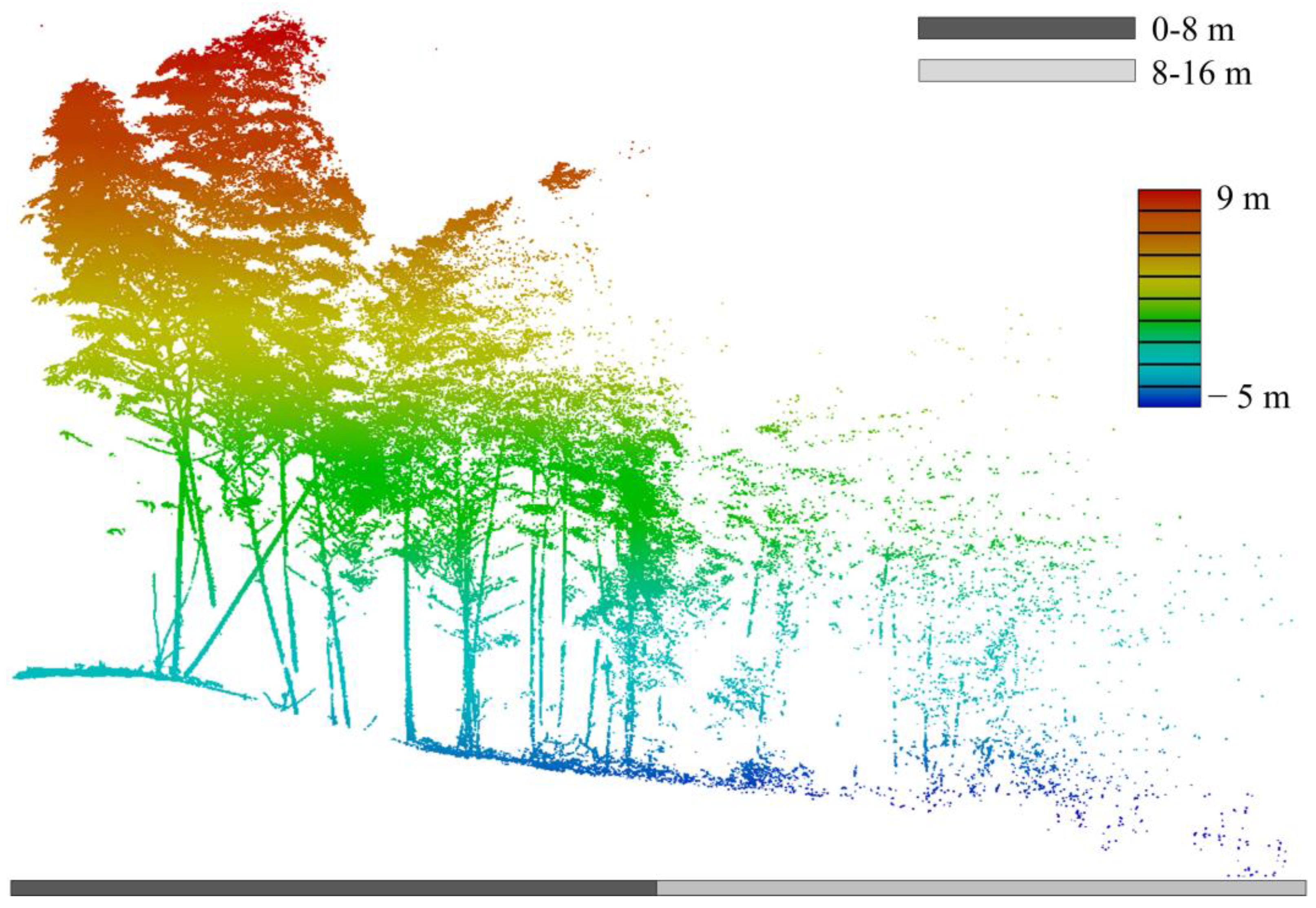
2. Study Area and Data

3. Methods
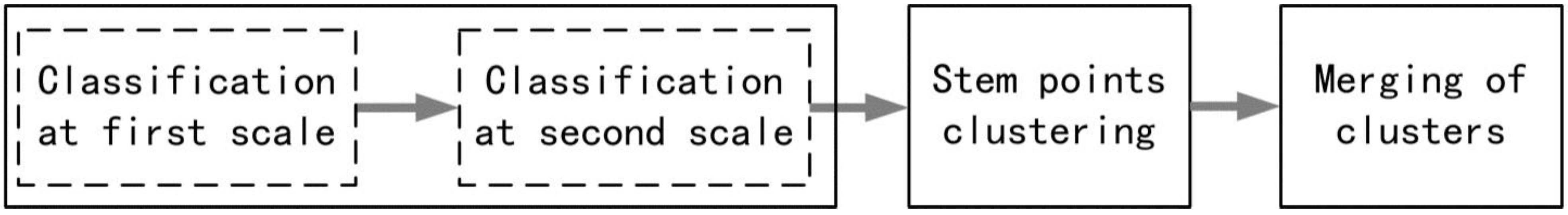
3.1. Two-Scale Classification
3.1.1. Multi-Scale Features of Vegetation Point Clouds

| Point clouds of stem (Height ≈ 80 cm, Radius ≈ 4 cm) |  |  |  |  |  |  |  |  |  |  |  |  |
| radius (cm) | 1 | 2 | 3 | 4 | 5 | 6 | 7 | 8 | 9 | 10 | 11 | 12 |
| linear (%) | 52.24 | 6.62 | 4.06 | 2.82 | 16.23 | 88.44 | 91.13 | 93.47 | 95.91 | 98.41 | 99.94 | 100 |
| planar (%) | 47.11 | 75.32 | 95.55 | 96.43 | 82.24 | 11.23 | 8.86 | 6.54 | 4.09 | 1.59 | 0.06 | 0 |
| Volumetric (%) | 0.65 | 18.06 | 0.39 | 0.75 | 1.43 | 0.33 | 0.01 | 0 | 0 | 0 | 0 | 0 |
| Branch | Foliage | Grass | Ground | |||||
|---|---|---|---|---|---|---|---|---|
| point number | 119 | 67,537 | 5996 | 7287 | ||||
| classified points |  |  | 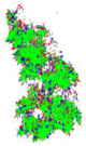 | 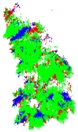 |  | 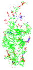 | 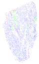 |  |
| dimensions (m) | 0.1/0.5 | 1.5/2.3 | 0.8/1.8 | 0.6/1.2 | ||||
| radius (cm) | 4 | 12 | 4 | 12 | 4 | 12 | 4 | 12 |
| linear (%) | 100 | 100 | 10.50 | 7.69 | 49.87 | 14.28 | 6.24 | 2.83 |
| planar (%) | 0 | 0 | 11.49 | 13.27 | 16.84 | 5.85 | 84.29 | 97.17 |
| volumetric (%) | 0 | 0 | 78.01 | 79.04 | 33.29 | 79.87 | 9.47 | 0 |
3.1.2. Optimal Radius Selection
| Algorithm 1. Scale selection | ||
| Input: Point clouds P; Given interval Output: radius set R | ||
| for every point Pi ∈ P do | ||
| for every radius rj ∈ [r1, ru] do | ||
| Find the neighboring points set sj of pi with . Calculate geometric features according to Equation (1). Calculate and record the entropy function Ej according to Equation (2). | ||
| end for | ||
| The radius rmin with minimal Emin is selected as the optimal radius for . Add rmin to R. | ||
| end for | ||
3.1.3. Candidate Stem Points Recognition
| Algorithm 2. Two-scale classification | |
| Input: Point clouds P; Given intervals [r1, r2] and [r3, r4] Output: Candidate stem point set Pstem | |
| (1) Run Algorithm 1 with interval [r1, r2], get optimal radiuses for all points. | |
| (2) Classify each point into linear, planar or volumetric according to Equation (1). | |
| (3) Only “planar” points remain | |
| (4) Run Algorithm 1 with interval [r3, r4], get optimal radiuses for remaining points. | |
| (5) Classify these points into linear, planar or volumetric according to Equation (1). | |
| (6) These “linear” points are recognized as candidate stem points Pstem | |
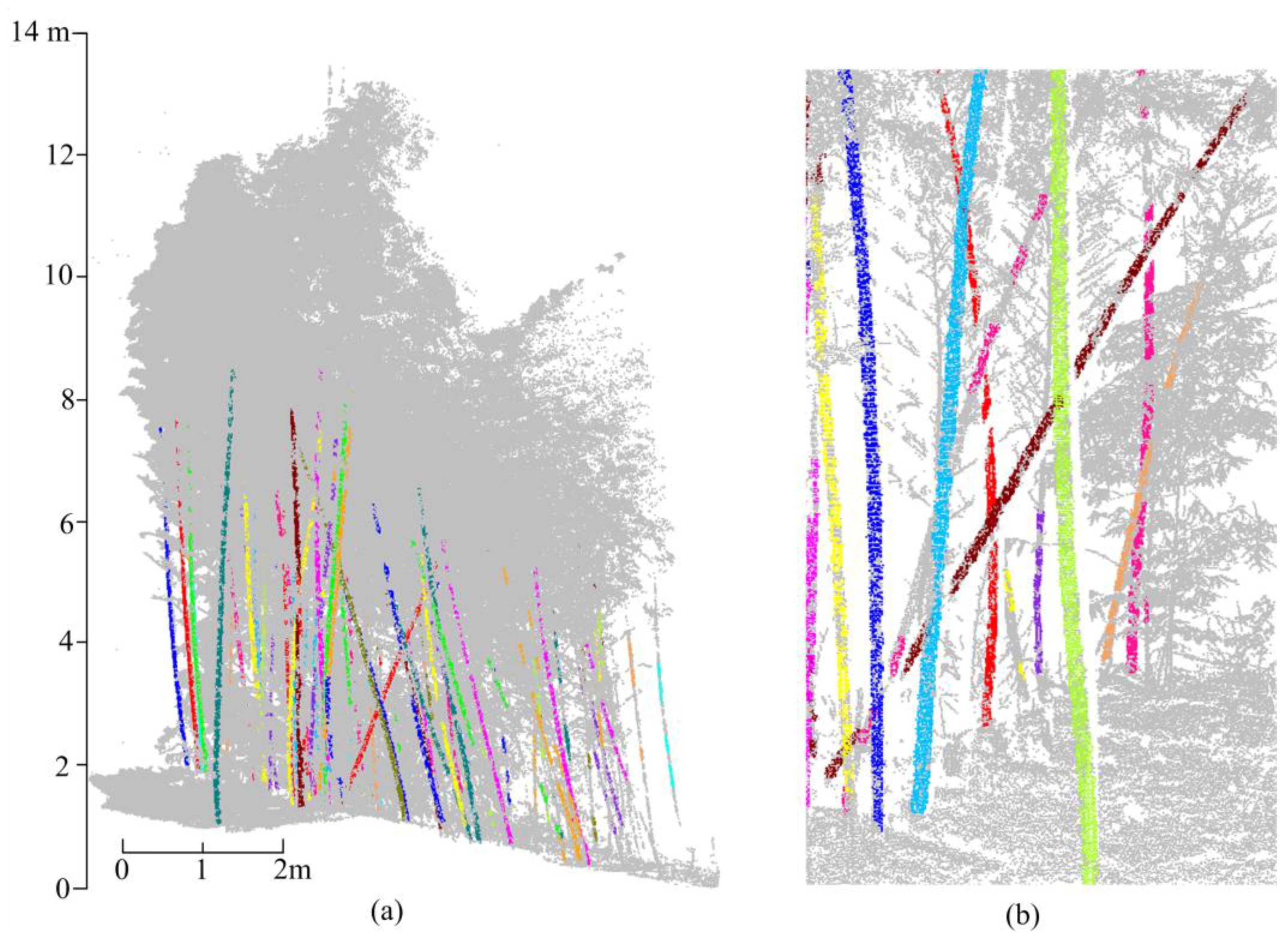
3.2. Clustering
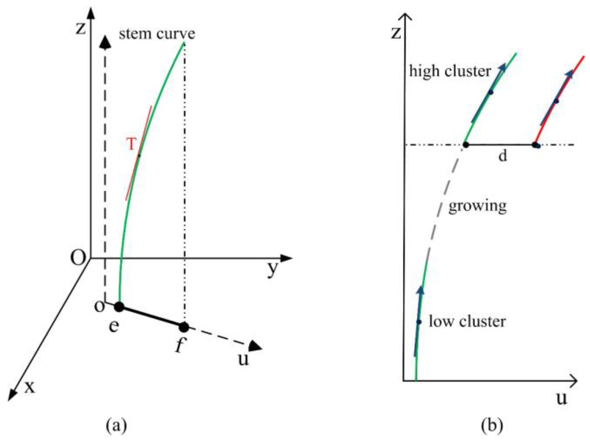
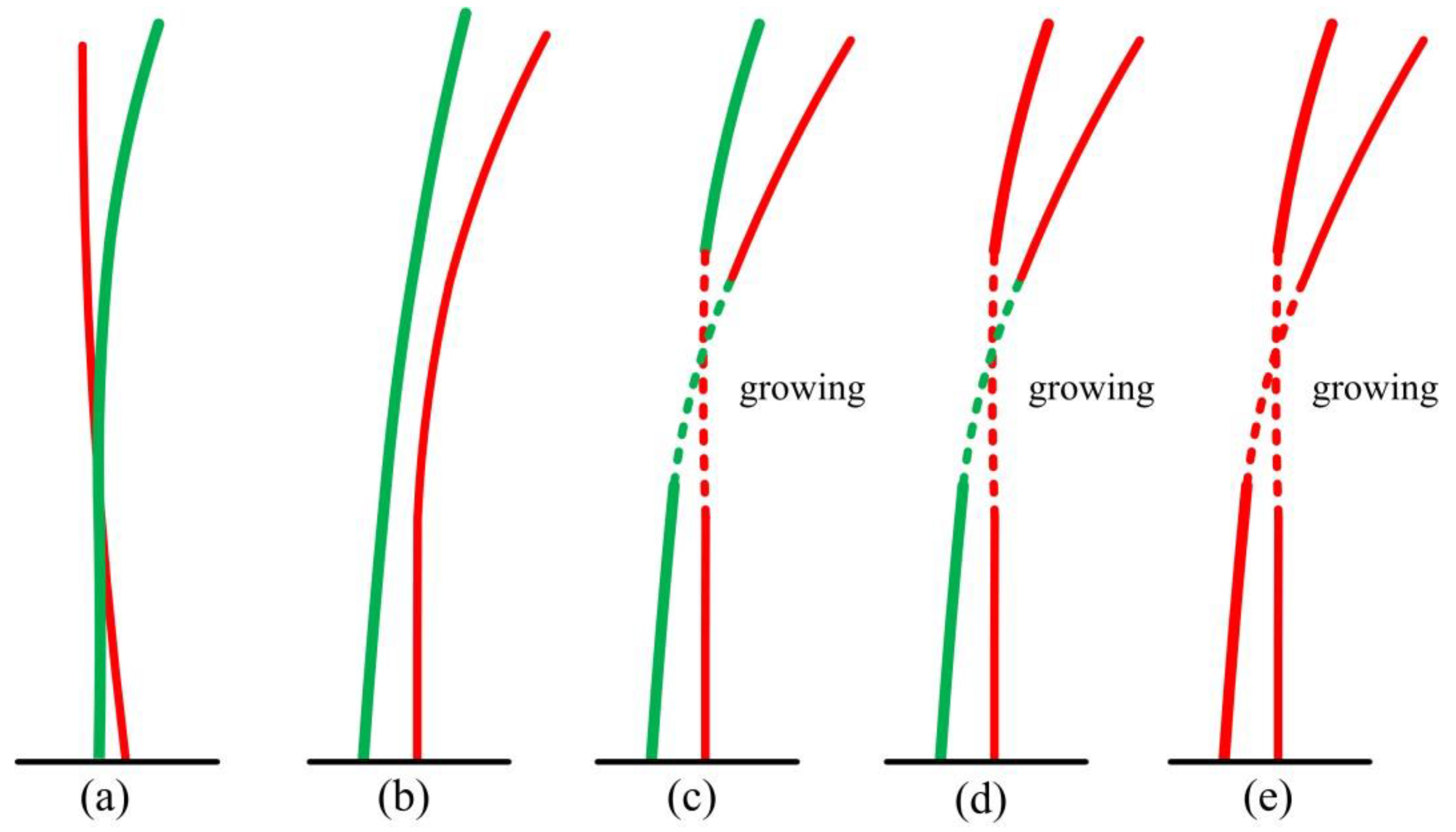
3.3. Merging Stem Clusters

| Algorithm 3. Merging of stem clusters | |||
| Input: points clusters C Output: stems list Cs | |||
| Initialize an empty list of Cs | |||
| for every cluster ci ∈ C do | |||
| for every stem csj ∈ Cs do | |||
| find the cluster ck ∈ csj which is nearest to ci calculate the direction vectors of ck and ci | |||
| solve parameters of linear models in Equation (9) using two direction vectors | |||
| growing of the seed point according to Equation (10) until it meets the higher cluster | |||
| if distance (ck, ci) < dstem then | |||
| add ci to csj; break; | |||
| end if | |||
| end for | |||
| if ci is not added to any csj ∈ Cs then | |||
| create a new stem and add it to Cs | |||
| end if | |||
| end for | |||
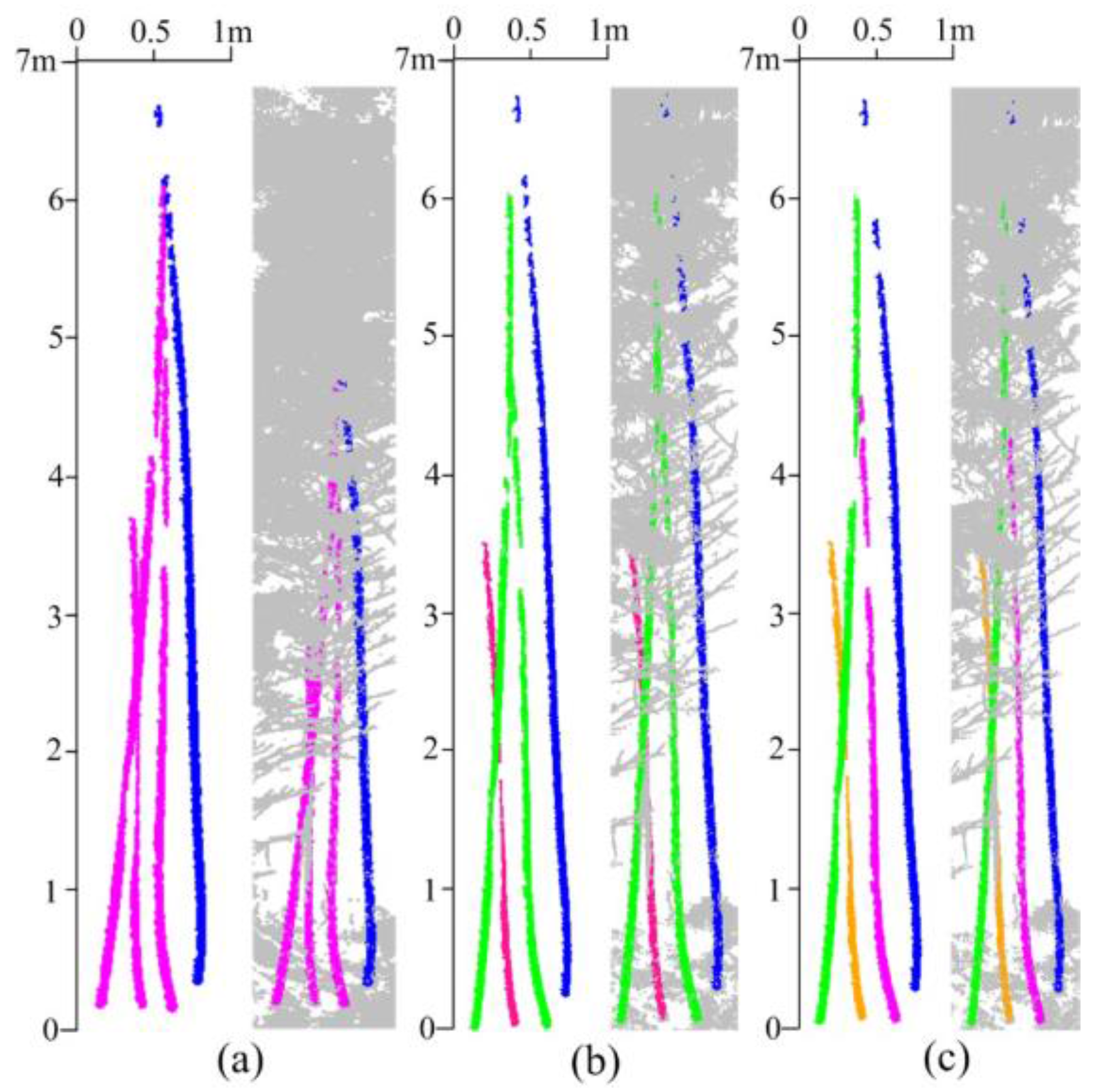
4. Experiments and Results
| Original | First Scale Classified | Second Scale Classified | Clustering | Merging | |
|---|---|---|---|---|---|
| Plot A | 3,384,528 | 1,095,781 | 551,077 | 340,133 | 329,417 |
| Plot B | 3,050,403 | 995,032 | 494,154 | 283,083 | 280,335 |
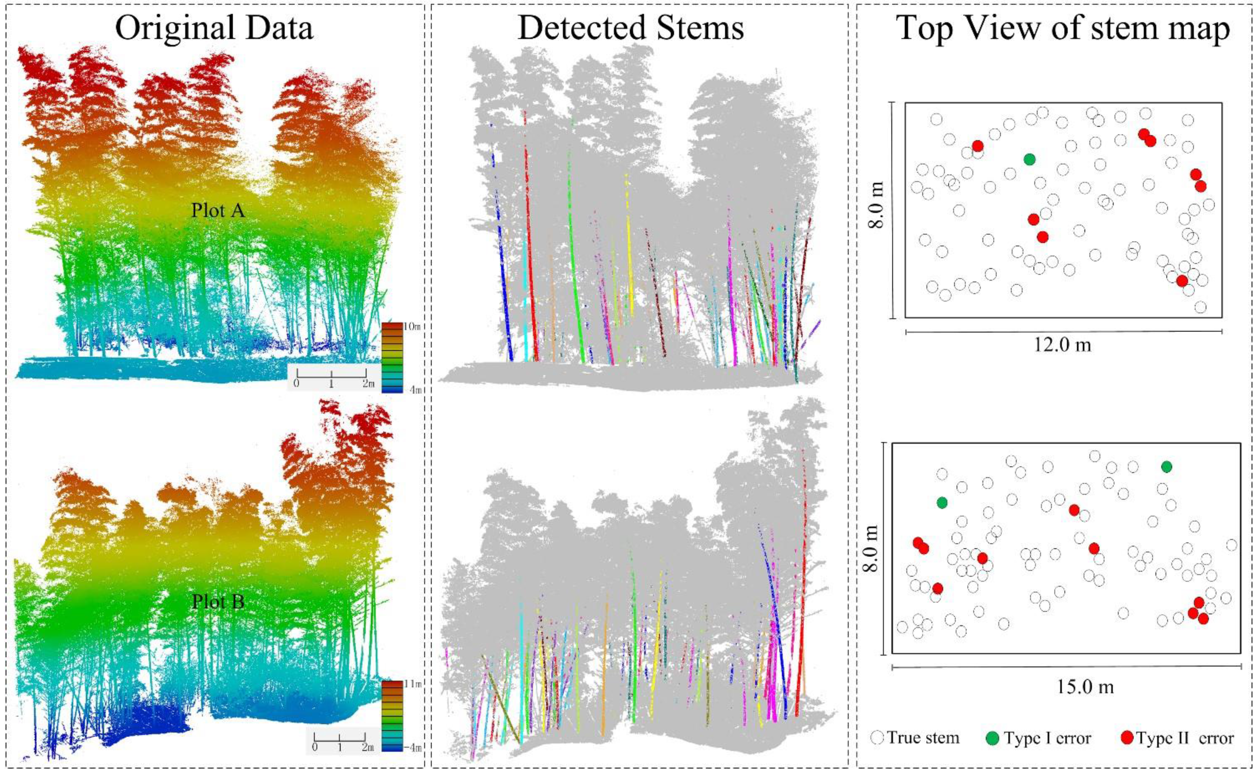
| Reference Bamboos | Detected Culms | Type I Error | Type II Error | True Culms | Completeness | |
|---|---|---|---|---|---|---|
| A | 82 | 78 | 1 | 5 | 73 | 89% |
| B | 84 | 79 | 2 | 6 | 73 | 86.9% |
| Total | 166 | 157 | 3 | 11 | 146 | 88.0% |
5. Discussion
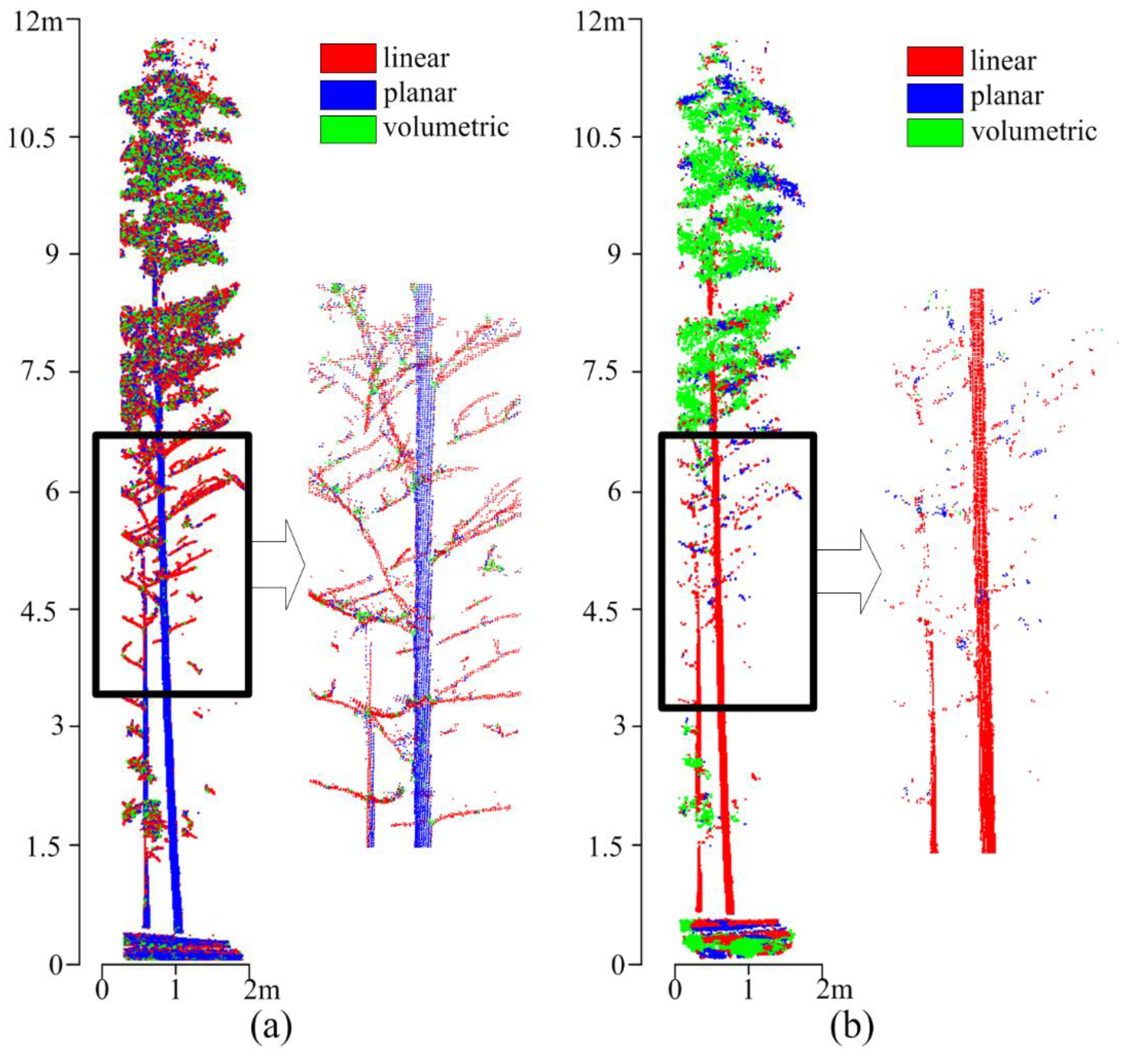
5.1. Stem Points Identification and Type I Error

5.2. Clusters Merging and Type II Error
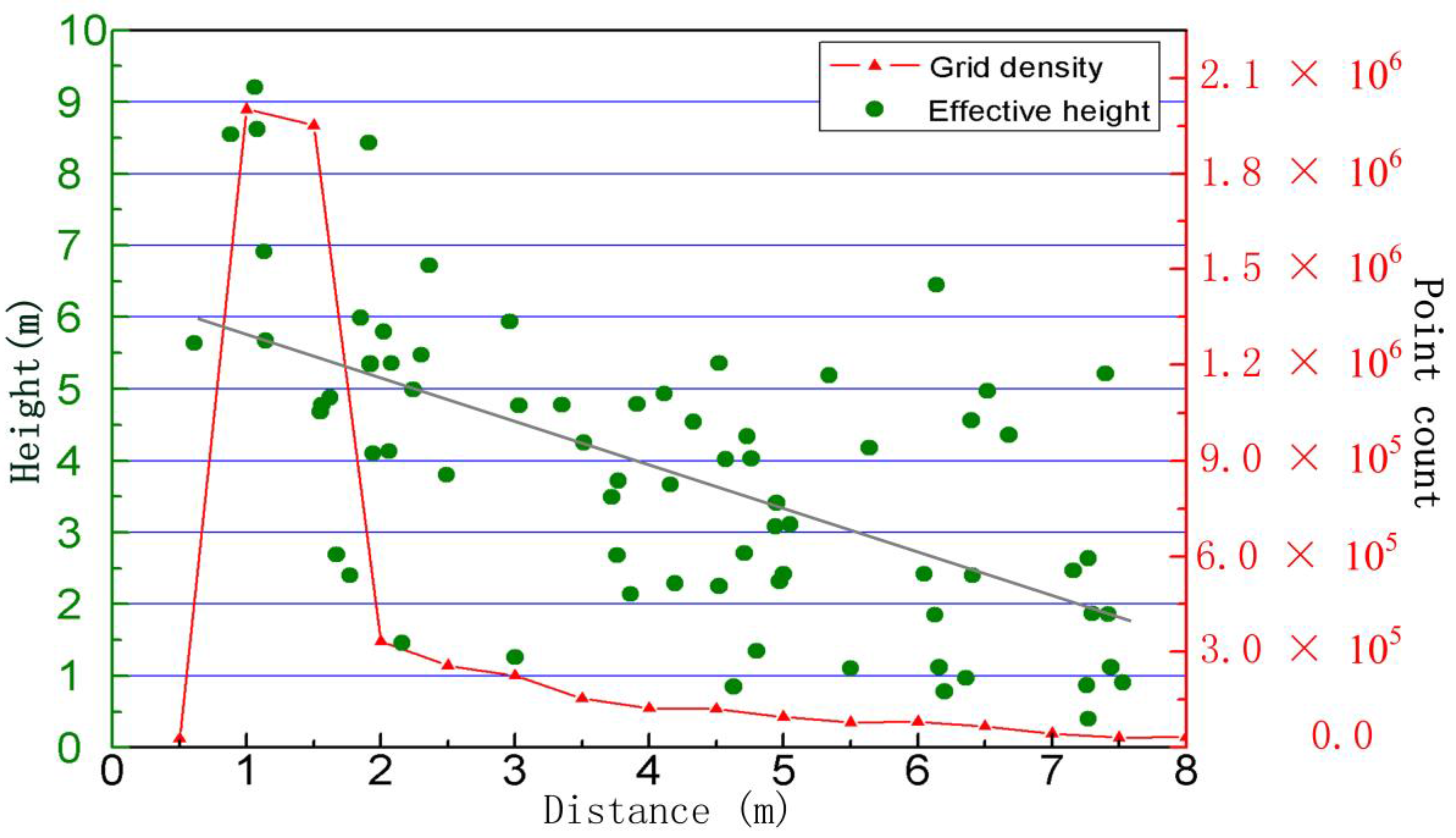
5.3. Measuring Range and Quality Assessment
| He (m) | <2.0 | 2.0–3.0 | 3.0–4.0 | 4.0–5.0 | 5.0–6.0 | 6.0–7.0 | >7.0 | Sum |
|---|---|---|---|---|---|---|---|---|
| Plot A | 15 | 13 | 7 | 19 | 12 | 3 | 4 | 73 |
| Plot B | 10 | 14 | 11 | 18 | 10 | 6 | 4 | 73 |
| Total | 25 | 27 | 18 | 37 | 22 | 9 | 8 | 146 |
| Percentage | 17.1% | 18.5% | 12.3% | 25.3% | 15.1% | 6.2% | 5.5% |
6. Conclusions
Acknowledgments
Author Contributions
Conflicts of Interest
References
- Chen, X.; Zhang, X.; Zhang, Y.; Booth, T.; He, X. Changes of carbon stocks in bamboo stands in china during 100 years. For. Ecol. Manag. 2009, 258, 1489–1496. [Google Scholar] [CrossRef]
- Yen, T.-M.; Ji, Y.-J.; Lee, J.-S. Estimating biomass production and carbon storage for a fast-growing makino bamboo (Phyllostachys makinoi) plant based on the diameter distribution model. For. Ecol. Manag. 2010, 260, 339–344. [Google Scholar] [CrossRef]
- Li, W.; Niu, Z.; Gao, S.; Huang, N.; Chen, H. Correlating the horizontal and vertical distribution of lidar point clouds with components of biomass in a picea crassifolia forest. Forests 2014, 5, 1910–1930. [Google Scholar] [CrossRef]
- Maltamo, M.; Eerikäinen, K.; Packalén, P.; Hyyppä, J. Estimation of stem volume using laser scanning-based canopy height metrics. Forestry 2006, 79, 217–229. [Google Scholar] [CrossRef]
- Liang, X.; Kankare, V.; Yu, X.; Hyyppa, J.; Holopainen, M. Automated stem curve measurement using terrestrial laser scanning. IEEE Trans. Geosci. Remote Sens. 2014, 52, 1739–1748. [Google Scholar] [CrossRef]
- Luo, S.; Wang, C.; Li, G.; Xi, X. Retrieving leaf area index using ICESat/GLAS full-waveform data. Remote Sens. Lett. 2013, 4, 745–753. [Google Scholar] [CrossRef]
- Wang, C.; Glenn, N.F. A linear regression method for tree canopy height estimation using airborne lidar data. Can. J. Remote Sens. 2008, 34 (sup2), S217–S227. [Google Scholar] [CrossRef]
- Liang, X.; Litkey, P.; Hyyppa, J.; Kaartinen, H.; Vastaranta, M.; Holopainen, M. Automatic stem mapping using single-scan terrestrial laser scanning. IEEE Trans. Geosci. Remote Sens. 2012, 50, 661–670. [Google Scholar] [CrossRef]
- Yang, X.; Strahler, A.H.; Schaaf, C.B.; Jupp, D.L.; Yao, T.; Zhao, F.; Wang, Z.; Culvenor, D.S.; Newnham, G.J.; Lovell, J.L. Three-dimensional forest reconstruction and structural parameter retrievals using a terrestrial full-waveform lidar instrument (echidna®). Remote Sens. Environ. 2013, 135, 36–51. [Google Scholar] [CrossRef]
- Zheng, G.; Moskal, L.M.; Kim, S.-H. Retrieval of effective leaf area index in heterogeneous forests with terrestrial laser scanning. IEEE Trans. Geosci. Remote Sens. 2013, 51, 777–786. [Google Scholar] [CrossRef]
- Liang, X.; Hyyppa, J.; Kukko, A.; Kaartinen, H.; Jaakkola, A.; Yu, X. The use of a mobile laser scanning system for mapping large forest plots. IEEE Geosci. Remote Sens. Lett. 2014, 11, 1504–1508. [Google Scholar] [CrossRef]
- Astrup, R.; Ducey, M.J.; Granhus, A.; Ritter, T.; von Lüpke, N. Approaches for estimating stand-level volume using terrestrial laser scanning in a single-scan mode. Can. J. For. Res. 2014, 44, 666–676. [Google Scholar] [CrossRef]
- Olofsson, K.; Holmgren, J.; Olsson, H. Tree stem and height measurements using terrestrial laser scanning and the ransac algorithm. Remote Sens. 2014, 6, 4323–4344. [Google Scholar] [CrossRef]
- Maas, H.G.; Bienert, A.; Scheller, S.; Keane, E. Automatic forest inventory parameter determination from terrestrial laser scanner data. Int. J. Remote Sens. 2008, 29, 1579–1593. [Google Scholar] [CrossRef]
- McDaniel, M.W.; Nishihata, T.; Brooks, C.A.; Salesses, P.; Iagnemma, K. Terrain classification and identification of tree stems using ground-based lidar. J. Field Robot. 2012, 29, 891–910. [Google Scholar] [CrossRef]
- Pfeifer, N.; Gorte, B.; Winterhalder, D. Automatic reconstruction of single trees from terrestrial laser scanner data. In Proceedings of the 20th ISPRS Congress, Istanbul, Turkey, 12 July, 2004; pp. 114–119.
- Bienert, A.; Schneider, D. Range image segmentation for tree detection in forest scans. In International Archives of the Photogrammetry, Remote Sensing and Spatial Information Sciences; Copernicus GmbH: Antalya, Turkey, 2013; Volume 5, pp. 49–54. [Google Scholar]
- Hetti Arachchige, N. Automatic tree stem detection—A geometric feature based approach for mls point clouds. In ISPRS Annals of Photogrammetry, Remote Sensing and Spatial Information Sciences; Copernicus GmbH: Antalya, Turkey, 2013; Volume 1, pp. 109–114. [Google Scholar]
- Lehtomäki, M.; Jaakkola, A.; Hyyppä, J.; Kukko, A.; Kaartinen, H. Detection of vertical pole-like objects in a road environment using vehicle-based laser scanning data. Remote Sens. 2010, 2, 641–664. [Google Scholar] [CrossRef]
- D’Oliveira, M.V.; Guarino, E.D.S.; Oliveira, L.C.; Ribas, L.A.; Acuña, M.H. Can forest management be sustainable in a bamboo dominated forest? A 12-year study of forest dynamics in western amazon. For. Ecol. Manag. 2013, 310, 672–679. [Google Scholar] [CrossRef]
- Scurlock, J.; Dayton, D.; Hames, B. Bamboo: An overlooked biomass resource? Biomass Bioenergy 2000, 19, 229–244. [Google Scholar] [CrossRef]
- Song, J.; Wang, X.; Liao, Y.; Zhen, J.; Ishwaran, N.; Guo, H.; Yang, R.; Liu, C.; Chang, C.; Zong, X. An improved neural network for regional giant panda habitat suitability mapping: A case study in Ya’An prefecture. Sustainability 2014, 6, 4059–4076. [Google Scholar] [CrossRef]
- Lalonde, J.F.; Vandapel, N.; Huber, D.F.; Hebert, M. Natural terrain classification using three-dimensional ladar data for ground robot mobility. J. Field Robot. 2006, 23, 839–861. [Google Scholar] [CrossRef]
- Brodu, N.; Lague, D. 3D terrestrial lidar data classification of complex natural scenes using a multi-scale dimensionality criterion: Applications in geomorphology. ISPRS J. Photogramm. Remote Sens. 2012, 68, 121–134. [Google Scholar] [CrossRef]
- Bremer, M.; Wichmann, V.; Rutzinger, M. Eigenvalue and graph-based object extraction from mobile laser scanning point clouds. In ISPRS Annals of the Photogrammetry, Remote Sensing and Spatial Information Sciences; Copernicus GmbHPublisher: AntalyaCity, Turkey, 2013; Volume 5, pp. 55–60. [Google Scholar]
- Demantké, J.; Mallet, C.; David, N.; Vallet, B. Dimensionality based scale selection in 3D lidar point clouds. In The International Archives of the Photogrammetry, Remote Sensing and Spatial Information Sciences; Copernicus GmbHPublisher: Calgary, Canada, 2011; pp. 97–102. [Google Scholar]
- Van Leeuwen, M.; Coops, N.C.; Hilker, T.; Wulder, M.A.; Newnham, G.J.; Culvenor, D.S. Automated reconstruction of tree and canopy structure for modeling the internal canopy radiation regime. Remote Sens. Environ. 2013, 136, 286–300. [Google Scholar] [CrossRef]
- Yang, B.; Dong, Z. A shape-based segmentation method for mobile laser scanning point clouds. ISPRS J. Photogramm. Remote Sens. 2013, 81, 19–30. [Google Scholar] [CrossRef]
- Gressin, A.; Mallet, C.; Demantké, J.; David, N. Towards 3D lidar point cloud registration improvement using optimal neighborhood knowledge. ISPRS J. Photogramm. Remote Sens. 2013, 79, 240–251. [Google Scholar] [CrossRef]
- Seidel, D.; Ammer, C. Efficient measurements of basal area in short rotation forests based on terrestrial laser scanning under special consideration of shadowing. iForest Biogeosci. For. 2014, 7, 227–232. [Google Scholar] [CrossRef]
- Seidel, D.; Albert, K.; Ammer, C.; Fehrmann, L.; Kleinn, C. Using terrestrial laser scanning to support biomass estimation in densely stocked young tree plantations. Int. J. Remote Sens. 2013, 34, 8699–8709. [Google Scholar] [CrossRef]
- Liang, X.; Wang, Y.; Jaakkola, A.; Kukko, A.; Kaartinen, H.; Hyyppa, J.; Honkavaara, E.; Jingbin, L. Forest Data Collection Using Terrestrial Image-Based Point Clouds From a Handheld Camera Compared to Terrestrial and Personal Laser Scanning. IEEE Trans. Geosci. Remote Sens. 2015, 53, 5132–5117. [Google Scholar] [CrossRef]
© 2015 by the authors; licensee MDPI, Basel, Switzerland. This article is an open access article distributed under the terms and conditions of the Creative Commons Attribution license (http://creativecommons.org/licenses/by/4.0/).
Share and Cite
Xia, S.; Wang, C.; Pan, F.; Xi, X.; Zeng, H.; Liu, H. Detecting Stems in Dense and Homogeneous Forest Using Single-Scan TLS. Forests 2015, 6, 3923-3945. https://doi.org/10.3390/f6113923
Xia S, Wang C, Pan F, Xi X, Zeng H, Liu H. Detecting Stems in Dense and Homogeneous Forest Using Single-Scan TLS. Forests. 2015; 6(11):3923-3945. https://doi.org/10.3390/f6113923
Chicago/Turabian StyleXia, Shaobo, Cheng Wang, Feifei Pan, Xiaohuan Xi, Hongcheng Zeng, and He Liu. 2015. "Detecting Stems in Dense and Homogeneous Forest Using Single-Scan TLS" Forests 6, no. 11: 3923-3945. https://doi.org/10.3390/f6113923
APA StyleXia, S., Wang, C., Pan, F., Xi, X., Zeng, H., & Liu, H. (2015). Detecting Stems in Dense and Homogeneous Forest Using Single-Scan TLS. Forests, 6(11), 3923-3945. https://doi.org/10.3390/f6113923