Estimating Soil Displacement from Timber Extraction Trails in Steep Terrain: Application of an Unmanned Aircraft for 3D Modelling

Abstract

Skid trails constructed for timber extraction in steep terrain constitute a serious environmental concern if not well planned, executed and ameliorated. Carrying out post-harvest surveys in monitoring constructed trails in such terrain is an onerous task for forest administrators, as hundreds of meters need to be surveyed per site, and the quantification of parameters and volumes is largely based on assumptions of trail symmetry and terrain uniformity. In this study, aerial imagery captured from a multi-rotor Unmanned Aerial Vehicle was used in generating a detailed post-harvest terrain model which included all skid trails. This was then compared with an Airborne Laser Scanning derived pre-harvest terrain model and the dimensions, slopes and cut-and-fill volumes associated with the skid trails were determined. The overall skid trail length was 954 m, or 381 m·ha⁻¹ with segments varying from 40–60 m, inclinations from 3.9% to 9.6%, and cut volumes, from 1.7 to 3.7 m³ per running meter. The methods used in this work can be used in rapidly assessing the extent of disturbance and erosion risk on a wide range of sites. The multi-rotor Unmanned Aerial Vehicle (UAV) was found to be highly suited to the task, given the relatively small size of harvested stands, their shape and their location in the mountainous terrain.

1. Introduction

Forest roads and skid trails are an acknowledged source of erosion and sedimentation in catchment areas, and have been a matter of research concern since the 1950s [1]. While the use of skid trails in timber extraction is often essential, they mostly comprise limited surface disturbance arising from the timber having been dragged by a skidder, and can be easily ameliorated. In steeper terrain a bulldozer or skidder with dozer blade is used in providing temporary access to machines, resulting in more drastic changes to the terrain. This practice and its associated problems, has been documented in western [1] and eastern USA [2,3,4,5], in Japan [6], Malaysia [7,8] and Australia [9,10,11].

By definition, skid trails have no constructed drainage or compacted road bed. This leads to a risk of collapsing cut-banks, downslope wash of un-compacted fill material, or redirected surface flows which confluence at intersections. These effects are cause for concern. Therefore there is an interest in knowing how much soil is disturbed in the construction of the trails, as well as their length and overall geometry, in evaluating the need for, and extent of, ameliorative measures.

In Norway, there are currently around 175 million m³ of timber mature or maturing in steep terrain (>33% slope) [12]. These slopes are traditionally harvested using cable based systems, in which a tree is partially or fully suspended in the air and carried out to a landing. However, a more rudimentary method involves using a ground-based harvester working alternately with an excavator, which opens temporary access trails and thereby provides access to machines on steep side slopes (Figure 1). The method, which requires ensuing extraction of the timber by forwarder, is fully mechanized and alleviates the difficult problem of recruiting people for the strenuous motor manual work that is synonymous with cable logging. Lileng [13] provides a more detailed explanation of this harvesting system which shows productivity figures of around 15 m³ per system hour, which is approximately double of what would be expected from cable yarders in similar terrain [14]. Thus there is a strong incentive for industry to continue to expand the use of this method in keeping costs in check, while accessing volumes that far exceed the capacity of the limited number of cable yarders in the country.

Estimates of soil displacement have been carried out visually along a transect [15], through measurement of stream turbidity [16] and through the use of sediment traps [10]. However, the advent of airborne laser scanning (ALS) has allowed for semi-automated volume calculations to be carried out along an intended road line. Examples are given by Aruga et al. [17] who aimed to minimize sedimentation through improved road design, and Contreras et al. [18] who apply road design geometry to an ALS derived Digital Elevation Model (DEM) in estimating earthwork requirements continuously. Related work employing ALS is the mapping of gullies and headwater streams [19] and the estimation of gully erosion [20].

As harvesting sites are often small and scattered, but difficult to access due to the nature of the terrain, remote measuring of the hillside using an Unmanned Aerial Vehicle (UAV) is an attractive option. However, forested steep terrain is associated with difficult flying conditions, both with regard to launch and landing sites, but also because of the vigilance needed in avoiding terrain. Unmanned Aerial Systems (UAS), involving the use of different platforms for airborne image acquisition, have recently become a widely applied technology due to their cost effectiveness compared with traditional airborne methods. The variety of UAV’s on offer, ease of operation, together with powerful computer vision algorithms for image processing, provides an easily accessible research tool. These allow for time flexible data acquisition on small specific sites, enabling spatial-temporal analyses of alterations in terrain. As light-weight LiDAR scanners are only just becoming commercially available, data acquisition from UAVs is commonly based on digital imagery.

Figure 1. Image of one of the skid trails, indicating how the material on the cut bank was already collapsing to a natural angle of repose by the time of the study.

Figure 1. Image of one of the skid trails, indicating how the material on the cut bank was already collapsing to a natural angle of repose by the time of the study.

Recent developments in computer vision enhanced the process of 3D model generation. Images from UAV’s mostly come from consumer-grade cameras, not initially designed for metric purposes, which is why interior orientation (IO) parameters are usually not known or inaccurate. Also, exterior camera orientation (EO) is less accurate for UAV platforms due to limited accuracy GPS and the Micro Electro Mechanical System’s (MEMS) Inertial Measurement Unit (IMU) [21]. In order to compensate for these shortcomings a sophisticated processing workflow is applied using Structure from Motion (SFM). This makes it possible to determine the scene geometry, camera calibration, position and orientation from an unordered, overlapping collection of images [22]. It makes use of Scale Invariant Feature Transform (SIFT) which is a feature extractor that is applicable to UAV imagery due to its robustness to changes in rotation, scale and translation between images [23,24,25]. SFM has been successfully applied in reconstructing objects from images coming from different sources [26].

The objective of this study was to develop a method for, and test the suitability of, the use of an inexpensive hobbyist aircraft, combined with SFM technology and an existing LiDAR derived DTM, in estimating post-harvest soil displacement and skid trail geometry.

2. Materials and Methods

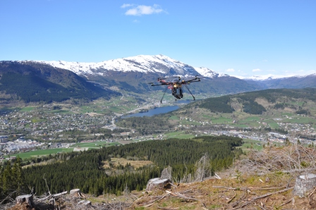
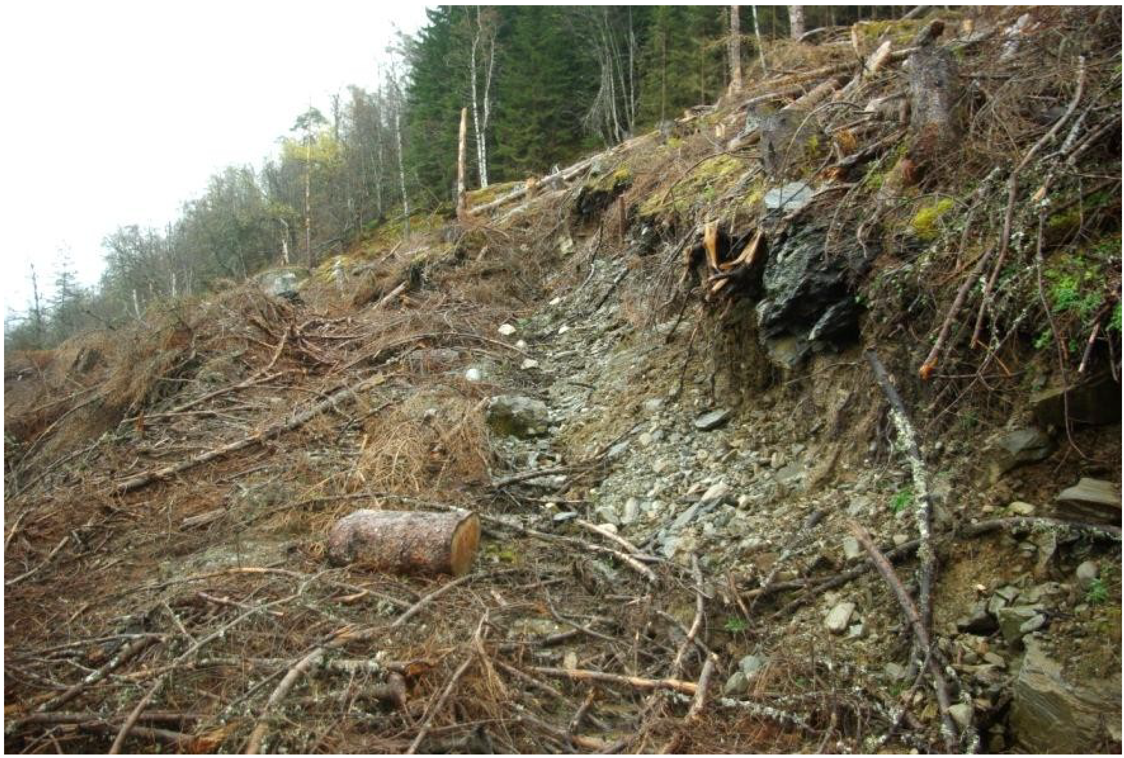
2.1. Study Site

A 7 ha forest stand in western Norway (UTM32-E 364,323 m, N 6,741,123 m) which had been harvested with the help of excavated skid trails was used as a case. The stand extended from 220 m above sea level at the lowest to roughly 400 m at the highest point. The slope had a northwesterly aspect, with an inclination of roughly 36% in the lower regions and approximately 55%–65% in the area where the trails had been excavated.

2.2. Data Acquisition

Six ground points were demarcated in the stand using fluorescent colored planks arranged in a V-shape at a 90° angle. Their positions were marked and positioned using differential GPS (DGPS) kinematic measurements.

For data acquisition we used photo imagery from a Sony NEX 5N camera (Table 1) mounted on an inexpensive hobbyist aircraft (IHA) [27], a Mikrokopter^® Okto 2-26. This UAV has 8 rotors and can lift up to 1 kg for flight duration of between 9 and 21 min depending on the type of LiPo battery [28].

Table 1. Details of the camera used on the MK Okto 2-26.

Manufacture and Model	Sony NEX-5N
Focal length, mm	16 (~24 on SLR)
Sensor size, mm	23.5 × 15.6
Resolution, pixels	4912 × 3264 (3:2)

Table 1. Details of the camera used on the MK Okto 2-26.

Manufacture and Model	Sony NEX-5N
Focal length, mm	16 (~24 on SLR)
Sensor size, mm	23.5 × 15.6
Resolution, pixels	4912 × 3264 (3:2)

The flight was carried out in early October 2013 in midafternoon. Light conditions were satisfactory, it was a sunny day and the slope was well illuminated over the whole area. The multi-rotor helicopter was controlled remotely and operated fully manually, flying up and down the slope. The aircraft was kept at a relatively constant height above the ground, following the terrain at a mean altitude of 155 m. The area of interest had a high overlap rate with at least nine images covering any point on the surface. Sixty seven images were selected for processing after manually removing those of worst quality (i.e., poor clarity). Also, the bulk of the images representing the lower part of the stand were excluded from the final analysis as no skid trails were constructed there. A terrain model was generated from the selected images using SFM technology. The validity of this approach is verified by [27] and [21] in providing satisfactory results Four skid trail sections of approx. 50 m in length were selected for detailed analysis. To verify the accuracy of the remotely sensed data, a high number of reference points were measured on the skid trails using DGPS with concurrent logging at a base station with radio frequency connection. Positions were recorded both for ground control points for surface model geo-correction (V-shaped points identifiable in the images) and the reference points for skid trail profiles. All these were recorded on the same day, logging concurrently from a base station located in direct line of sight in the opposite side of the valley, roughly 1200 m away. Reference points representing critical points for every skid road profile comprising such features as cut bank edges, road bed shoulders, as well as distinguishing features like wheel ruts, were recorded. These critical points were to be used as reference information on the photogrammetric model.

2.3. Data Processing

Image processing was conducted in compliance with photogrammetric workflow presented in Rossi, et al. [24] and Turner, et al. [29]. We used Agisoft Photoscan Professional^®software which employs full SFM-Multi View Stereopsis and estimates internal optical parameters and spatial positioning of the respective cameras [30]. Firstly, a sparse point cloud was generated by performing automatic photo alignment that retrieves camera positions. However, consumer grade cameras require calibration that can be performed in deriving camera intrinsic parameters [31]. While the software automatically calculates camera calibration parameters from EXIF (exchangeable image file format) metadata, it is possible to fit camera parameters in order to minimize the model distortion known as “bowl effect” using ground control points as a reference in a process known as camera optimization [32]. Geo-referencing is performed after a sparse point cloud is reconstructed, and done using ground control points where the whole model is transformed to the preselected coordinate system using Helmert transformation .This method is called ground control point (GCP) technique [21]. Based on the estimated camera positions the program calculates depth information based on the intersection of light rays between different camera stations, to be combined into a single dense point cloud. The ultimate result is an ultra-high resolution point cloud that is used for further analysis.

To calculate the soil displacement volumes, a pre-harvest ALS derived terrain model was to represent the terrain before the skid trails were constructed. The ALS was carried out on 4 September 2010 with a mean point spacing of 0.35 m. Confirmed ground points were exported and used as a reference layer representing the pre-harvest terrain. We used the ground point classification as set by the data provider, which resulted in a final spacing of 1.67 m between ground points.

2.4. Calculation of Soil Displacement

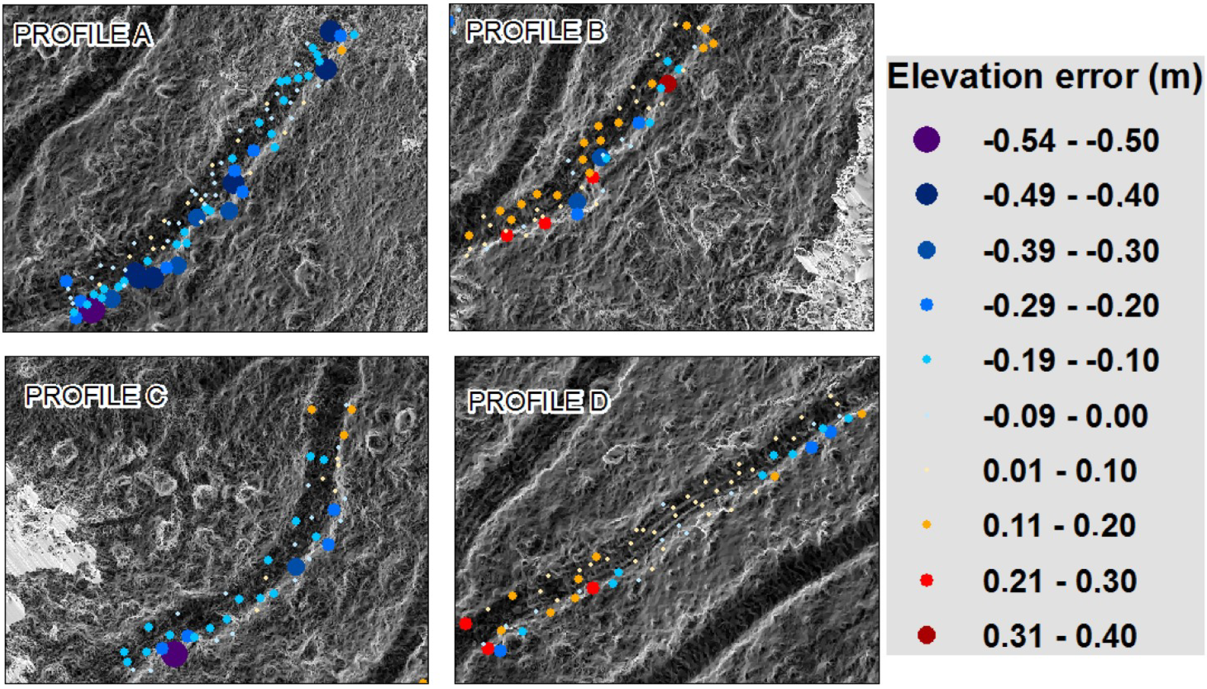
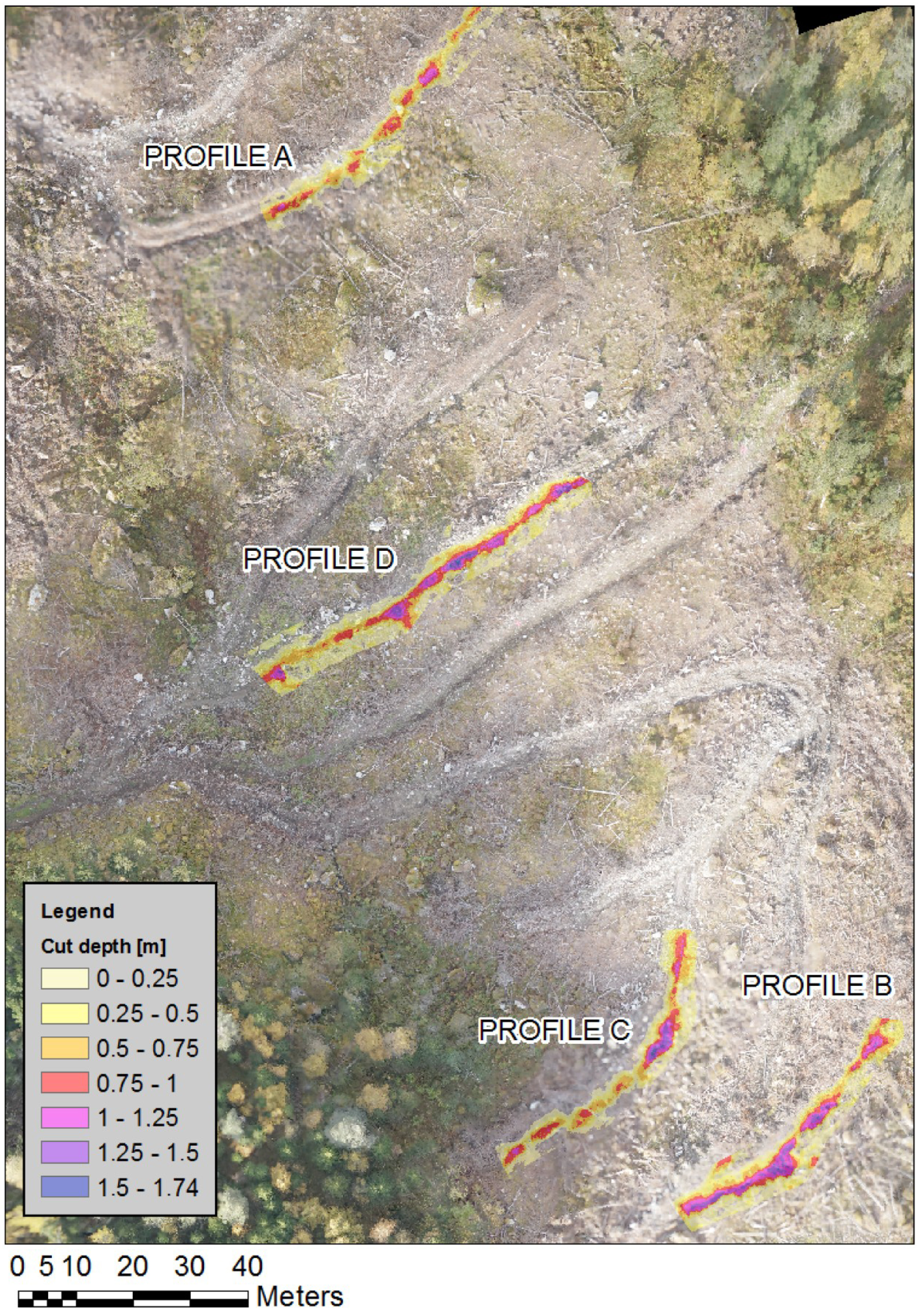
By comparing the surface models before and after the harvesting operation, estimates of the soil displacement volumes from skidding trails could be computed. The polygon area representing the selected sections was used to clip the points from an ultra-high resolution point cloud for further analysis. A regular grid point with a set resolution of 0.1 m was created within the area of interest. Attribute values representing elevation were assigned by location from the laser and photogrammetry point layer by applying the “add surface information” tool from 3D Analyst toolbox in ESRI’s ArcMap^®. Linear interpolation was used on the elevation, Z. Following that, an elevation difference calculation was done for every point. Positive difference represents a lower elevation of the photogrammetric post-harvest model compared to the pre-harvest laser ground surface. With known constant point spacing, it was also possible to calculate the differential volume contributing to every point, which was represented by a raster cell of 0.01 m². As a secondary control, the skid roads were also surveyed by applying the DGPS reference points from each profile. Those points were used as a control of elevation for the modelled profiles and the error was calculated by comparing their Z value with elevation of corresponding elevation model points. Also, reference points were used to study the influence of the elevation error on the soil volumes. For each profile a mean elevation error from DGPS was calculated and its value was subtracted from original elevation values for each profile grid point. Using the adjusted values, we calculated the new volume and then estimated the error influence. This influence was represented by the percentage volume change per 1 cm of adjustment of elevation value in each profile.

3. Results

The calculated digital terrain model had a total error of 0.082 m, after camera optimization. Outside the main study area (upper and lower stretches of the stand), there was notable peripheral bias, however this was eliminated before the analysis was carried out.

In total, it was estimated that some 554 m³ of earth had been displaced by the construction of skid trails over a cumulative length of 210 m, giving an average of over 2.6 m³ per running meter (Table 2). In the steepest part of the stand, the density of excavated trails was roughly 381 m·ha⁻¹, or 954 m length in total.

Table 2. Details on the road geometry and cut volumes, by profile.

	Profile A	Profile B	Profile C	Profile D
Reference point count/(subsampled)	93/69	62/44	48/31	67/48
Segment length, m	55	45	50	60
Reference point Elevation error, m	−0.09	0.03	−0.11	0.03
Standard deviation of elevation error, m	0.11	0.12	0.1	0.08
Min/Max DGPS elevation error, m	−0.49/0.05	−0.34/0.22	−0.37/0.12	−0.19/0.22
Cut volume, m3	94.43	166.48	117.2	176.34
Cut volume, m3·m−1	1.72	3.7	2.34	2.94
Side slope, %	45.3	56.8	47.9	49.0
Trail segment inclination, %	3.9	5.4	0.5	9.6

Table 2. Details on the road geometry and cut volumes, by profile.

	Profile A	Profile B	Profile C	Profile D
Reference point count/(subsampled)	93/69	62/44	48/31	67/48
Segment length, m	55	45	50	60
Reference point Elevation error, m	−0.09	0.03	−0.11	0.03
Standard deviation of elevation error, m	0.11	0.12	0.1	0.08
Min/Max DGPS elevation error, m	−0.49/0.05	−0.34/0.22	−0.37/0.12	−0.19/0.22
Cut volume, m3	94.43	166.48	117.2	176.34
Cut volume, m3·m−1	1.72	3.7	2.34	2.94
Side slope, %	45.3	56.8	47.9	49.0
Trail segment inclination, %	3.9	5.4	0.5	9.6

Positive volumetric values were observed possibly due to the presence of harvesting slash distributed over the whole site. Harvesting slash is also present directly on the skid trails in compacted form which is included in the skid trails surface models and visible in Figure 1. Most of the slash occurred at the end of the tracks where that mass was deposited by the machine.

The side slope (hill slope) immediately adjacent to the trails ranged between 45% and 57% and cut volume increased with side slope as could be expected from a purely geometric viewpoint.

DGPS error distribution varied across profiles where the mean average error for the respective segments is presented in Table 2. Some reference points showed a significant error on the Z value of over 50 cm. The most excessive disparities occurred in areas adjacent to a road bank, predominantly on the cut slope (Figure 2). All reference points at the top edge of the cut bank profile were assumed to have a high uncertainty owing to the abrupt terrain difference. Thus, out of the total 268 DGPS observations, we retained 192 points for further analysis. The subsampled dataset resulted in a reduced mean average error (Table 2).

Recalculated volumes with error correction are presented in Table 3. The recalculated profiles show a maximum change of 23% in the cut volume, or just over 2% per cm adjustment in the model.

Figure 2. The location of DGPS reference points with the elevation error in meters shown by their respective colors.

Figure 2. The location of DGPS reference points with the elevation error in meters shown by their respective colors.

Table 3. Details on the cut volumes after applying the mean error resulting from DGPS.

	Profile A	Profile B	Profile C	Profile D
Recalculated cut volume, m3	73.36	175.92	90.06	186.22
Recalculated cut volume, m3·m−1	1.33	3.9	1.8	3.1
Percent change	22%	−6%	23%	−6%
Percent change per 1cm elev.	2.28%	1.93%	2.01%	2.17%

Table 3. Details on the cut volumes after applying the mean error resulting from DGPS.

	Profile A	Profile B	Profile C	Profile D
Recalculated cut volume, m3	73.36	175.92	90.06	186.22
Recalculated cut volume, m3·m−1	1.33	3.9	1.8	3.1
Percent change	22%	−6%	23%	−6%
Percent change per 1cm elev.	2.28%	1.93%	2.01%	2.17%

4. Discussion

The spatial accuracy of the model, as provided by the Agisoft Photoscan^® processing report on the 6 GCP estimates was satisfactory, resulting in Total RMS error of (0.082 m). The detailed RMSE’s were X = 0.056 m, Y = 0.022 m, Z = 0.054 m. Turner et al. [21] showed a spatial accuracy of 0.129 and 0.103 m for the GCP technique for 25 and 20 ground control points respectively. However his study was not on a digital terrain model but geo-rectified mosaics.

The profiles with highest and lowest side slope (A and B) show the largest differences on soil volumes per running meter (Figure 3). Profile A was located on the lower part of the slope with side slope inclination around 45%. The upper slope section (profile B) has an inclination 11% greater, yet almost twice as much soil was displaced during its construction. This shows the strong influence of the slope inclination on the cut volume. In the steeper terrain, some uncontrolled soil displacement caused by formation of erosion gullies was modelled, mainly in profile B and C (e.g., center of Profile B in Figure 2).

Figure 3. Mosaicked orthophoto of the clearcut area with a semitransparent raster layer representing the depth of the soil cut in creating the skid trails.

Figure 3. Mosaicked orthophoto of the clearcut area with a semitransparent raster layer representing the depth of the soil cut in creating the skid trails.

The majority of the DGPS reference points established over the selected profiles showed a good fit with the modelled surface, most of which had a maximum deviation of a few centimeters. Those areas are located directly on skid trail surfaces. As the DGPS logging of both the GCPs and the elevation reference points was carried out simultaneously and from the same base station, it is possible that there was some degree of correlation between the resultant model and the reference points themselves. The highest bias was found on the upper edge points of the profile. Such a discrepancy could be explained in several ways. Firstly the abrupt break in terrain resulting from the skid trail is difficult to model precisely at the edges. It is also hard to preserve such textures when reconstructing the terrain from the images as the information is partially lost during the reconstruction process. The second reason is the spatial XY error of the model, which causes a shift in the critical points of the profile.

In this study we focused only on the cut volume as the assessment of fill volume is more difficult to model accurately, though it is assumed to be equal in total as no longitudinal transport of material takes place during construction. Determining fill volume is complicated by the fact that its bulk density is unknown, that the soil is mixed with harvest residues, that it is displaced over a larger downhill area especially in steep terrain, and objects such as boulders or stumps can have been made visible above the ALS terrain model.

Due to low laser penetration through the dense forest canopy, the ALS data was sparse in comparison to the very detailed surface information from UAV imagery. This weakened the benefit of the high resolution photogrammetry derived terrain model, where the overall model accuracy is limited to the poorest of the two. More accurate comparisons could be expected from forests with lower stand density and limited understory, allowing for a higher number of ground point returns on the ALS, and a better resolution match between that and the photogrammetry derived point cloud. Some information on micro-relief was lost during point classification of the ALS data by the data provider. The generation of a triangulated irregular network led to a simplification of the pre-harvesting terrain model and presumably affected the result negatively. Through the application of a regular grid, we extracted the interpolated surface information which was often some distance from the original laser point. This information could be improved by reclassifying the ground points.

The sparseness of the ALS ground point caused uncertainty in the volume estimates, but the generated point cloud also includes bias caused by other issues. Firstly, the model distortion which was impossible to remove completely but solely minimized by the camera optimization procedure has a significant influence on the estimate accuracy. It is very likely that within the area of interest which is concentrated within the central section of the stand, some minimal deflection is present. As the study shows, even a few centimeters of elevation difference greatly affects the volume estimates. DGPS reference points used here revealed that the model is not perfect. When considering the rate of change in volume estimate with fine increments in elevation it is seen that the model is relatively sensitive (ca. 2% per 1 cm increment). When taking the geo-correction error on Z value (5 cm) we can assume a 10% error on the soil volume estimate when neglecting other factors. A manual road survey, despite the inordinate amount of time and effort required, would likely be considerably less accurate as assumptions of uniformity and symmetry are used between stations. Any elevation error in this model is likely influenced by the very large elevation interval on the site, with a vertical difference of over 120 m between the lowest and highest points in modelled terrain.

5. Conclusions

The capture and analysis of remotely sensed data from a multi-rotor UAV for this application shows considerable potential for improved environmental management and associated cost reduction. The extent of fieldwork necessary in surveying a harvesting site in mountainous conditions is drastically reduced while both the quality and quantity of the information is significantly improved.

We show that it is possible to estimate soil displacement from skid trails using the images from an inexpensive hobbyist aircraft and the approach outlined here. As illustrated in this study, such an aircraft can provide a highly detailed terrain model at low cost. Such terrain models can potentially have a number of other uses, including hydrological and erosion modelling.

However for accurate estimation, the coverage area and flying altitude needs to be reduced due to model deflection that is distributed over the area. For obtaining better results, the camera should be precisely calibrated. Also, a more dense GCP distribution can be used for better geo-correction results and could also result in better optimization when not using a calibrated camera, especially when working in steep terrain.

References

1. Megahan, W.F.; Kidd, W.J. Effects of Logging and Logging Roads on Erosion and Sediment Deposition from Steep Terrain. J. For. 1972, 70, 136–141. [Google Scholar]
2. Smidt, M.F.; Kolka, R.K. Alternative Skid Trail Retirement Options for Steep Terrain Logging. In Appalachian Hardwoods: Managing Change, Proceedings of the 24th Annual Meeting of the Council of Forest Engineering (COFE), Snowshoe, WV, USA, 15–19 July 2001; Wang, J., Wolford, M., McNeel, J.F., Eds.; USDA Forest Service: Snowshoe, WV, USA, 2001; p. 6. [Google Scholar]
3. Christopher, E.A.; Visser, R. Methodology for Evaluating Post Harvest Erosion Risk for the Protection of Water Quality. N. Z. J. For. 2007, 52, 20–25. [Google Scholar]
4. Sawyers, B.C.; Bolding, M.C.; Aust, W.M.; Lakel, W.A. Effectiveness and Implementation Costs of Overland Skid Trail Closure Techniques in the Virginia Piedmont. J. Soil Water Conserv. 2012, 67, 300–310. [Google Scholar]
5. Worrell, W.C.; Bolding, M.C.; Aust, W.M. Potential Soil Erosion Following Skyline Yarding Versus Tracked Skidding on Bladed Skid Trails on the Appalachian Region of Virginia. South. J. Appl. For. 2011, 35, 131–135. [Google Scholar]
6. Kanzaki, K.; Ohasi, K.; Deki, T.; Miyake, T. On Capillary Path Systems in Steep Mountain Areas. Int. J. For. Eng. 1990, 2, 17–21. [Google Scholar]
7. Pinard, M.A.; Barker, M.G.; Tay, J. Soil Disturbance and Post-Logging Forest Recovery on Bulldozer Paths in Sabah, Malaysia. For. Ecol. Manag. 2000, 130, 213–225. [Google Scholar] [CrossRef]
8. Sidle, R.C.; Sasaki, S.; Otsuki, M.; Noguchi, S.; Rahim Nik, A. Sediment Pathways in a Tropical Forest: Effects of Logging Roads and Skid Trails. Hydrol. Process. 2004, 18, 703–720. [Google Scholar]
9. Webb, A.A.; Dragovich, D.; Jamshidi, R. Temporary Increases in Suspended Sediment Yields Following Selective Eucalypt Forest Harvesting. For. Ecol. Manag. 2012, 283, 96–105. [Google Scholar] [CrossRef]
10. Davies, P.E.; Nelson, M. The Effect of Steep Slope Logging on Fine Sediment Infiltration into the Beds of Ephemeral and Perennial Streams of the Dazzler Range, Tasmania, Australia. J. Hydrol. 1993, 150, 481–504. [Google Scholar] [CrossRef]
11. Cornish, P.M. The Effects of Roading, Harvesting and Forest Regeneration on Streamwater Turbidity Levels in a Moist Eucalypt Forest. For. Ecol. Manag. 2001, 152, 293–312. [Google Scholar] [CrossRef]
12. Granhus, A.; Hylen, G.; Nilsen, J.-E. Skogen i Norge: Statistikk over Skogforhold og Skogressurser i Norge Registrert i Perioden 2005–2009. In Statistics of Forest Conditions and Resources in Norway; Norwegian Forest and Landscape Institute: Ås, Norway, 2012; p. 85. [Google Scholar]
13. Lileng, J. Avvirkning med Hjulgående Maskiner i Bratt Terreng. In Harvesting with Ground Based Systems in Steep Terrain; Norwegian Forest and Landscape Institute: Ås, Norway, 2009; pp. 1–7. [Google Scholar]
14. Torgersen, H.; Lisland, T. Excavator-Based Cable Logging and Processing System: A Norwegian Case Study. Int. J. For. Eng. 2002, 13, 11–16. [Google Scholar]
15. McIver, J.D.; McNeil, R. Soil Disturbance and Hill-Slope Sediment Transport after Logging of a Severely Burned Site in Northeastern Oregon. West. J. Appl. For. 2006, 21, 123–133. [Google Scholar]
16. Wang, J.; Edwards, P.J.; Wood, F. Turbidity and Suspended-Sediment Changes from Stream-Crossing Construction on a Forest Haul Road in West Virginia, USA. Int. J. For. Eng. 2013, 24, 76–90. [Google Scholar]
17. Aruga, K.; Sessions, J.; Miyata, E.S. Forest Road Design with Soil Sediment Evaluation Using a High-Resolution Dem. J. For. Res. 2005, 10, 471–479. [Google Scholar] [CrossRef]
18. Contreras, M.; Aracena, P.; Chung, W. Improving Accuracy in Earthwork Volume Estimation for Proposed Forest Roads Using a High-Resolution Digital Elevation Model. Croat. J. For. Eng. 2012, 33, 125–142. [Google Scholar]
19. James, L.A.; Watson, D.G.; Hansen, W.F. Using Lidar Data to Map Gullies and Headwater Streams under Forest Canopy: South Carolina, USA. CATENA 2007, 71, 132–144. [Google Scholar] [CrossRef]
20. Perroy, R.L.; Bookhagen, B.; Asner, G.P.; Chadwick, O.A. Comparison of Gully Erosion Estimates Using Airborne and Ground-Based Lidar on Santa Cruz Island, California. Geomorphology 2010, 118, 288–300. [Google Scholar] [CrossRef]
21. Turner, D.; Lucieer, A.; Watson, C. An Automated Technique for Generating Georectified Mosaics from Ultra-High Resolution Unmanned Aerial Vehicle (UAV) Imagery, Based on Structure From Motion (SFM) Point Clouds. Remote Sens. 2012, 4, 1392–1410. [Google Scholar] [CrossRef]
22. Lisein, J.; Pierrot-Deseilligny, M.; Bonnet, S.; Lejeune, P. A Photogrammetric Workflow for the Creation of a Forest Canopy Height Model from Small Unmanned Aerial System Imagery. Forests 2013, 4, 922–944. [Google Scholar] [CrossRef]
23. Lingua, A.; Marenchino, D.; Nex, F. Performance Analysis of the Sift Operator for Automatic Feature Extraction and Matching in Photogrammetric Applications. Sensors 2009, 9, 3745–3766. [Google Scholar] [CrossRef]
24. Rossi, A.J.; Rhody, H.; Salvaggio, C.; Walvoord, D.J. Abstracted Workflow Framework with a Structure from Motion Application. In Proceedings of Image Processing Workshop (WNYIPW), New York, NY, USA, 9 November 2012; pp. 9–12.
25. Lowe, D. Distinctive Image Features from Scale-Invariant Keypoints. Int. J. Comput. Vis. 2004, 60, 91–110. [Google Scholar] [CrossRef]
26. Snavely, N.; Seitz, S.M.; Szeliski, R. Photo Tourism: Exploring Photo Collections in 3D. ACM Trans. Graphics 2006, 25, 835–846. [Google Scholar] [CrossRef]
27. Dandois, J.P.; Ellis, E.C. Remote Sensing of Vegetation Structure Using Computer Vision. Remote Sens. 2010, 2, 1157–1176. [Google Scholar] [CrossRef]
28. Flight Time of Mikrokopters. Available online: http://www.mikrokopter.de/ucwiki/en/FlightTime#MikroKopter_as_Okto_.2BAC8_Okto2 (accessed on 9 April 2014).
29. Turner, D.; Lucieer, A.; Wallace, L. Direct Georeferencing of Ultrahigh-Resolution UAV Imagery. Geosci. Remote Sens. IEEE Trans. 2014, 52, 2738–2745. [Google Scholar] [CrossRef]
30. Verhoeven, G. Taking Computer Vision Aloft—Archaeological Three-Dimensional Reconstructions from Aerial Photographs with Photoscan. Archaeol. Prospec. 2011, 18, 67–73. [Google Scholar] [CrossRef]
31. Bouguet, J.-Y. Camera calibration toolbox for matlab. 2004. Available online: http://www.vision.caltech.edu/bouguetj/calib_doc/ (accessed on 30 January 2014).
32. Agisoft Online Help for Agisoft Photoscan Professional. Available online: http://www.agisoft.ru/tutorials/photoscan (accessed on 8 April 2014).