Tree Root System Characterization and Volume Estimation by Terrestrial Laser Scanning and Quantitative Structure Modeling

Abstract

The accurate characterization of three-dimensional (3D) root architecture, volume, and biomass is important for a wide variety of applications in forest ecology and to better understand tree and soil stability. Technological advancements have led to increasingly more digitized and automated procedures, which have been used to more accurately and quickly describe the 3D structure of root systems. Terrestrial laser scanners (TLS) have successfully been used to describe aboveground structures of individual trees and stand structure, but have only recently been applied to the 3D characterization of whole root systems. In this study, 13 recently harvested Norway spruce root systems were mechanically pulled from the soil, cleaned, and their volumes were measured by displacement. The root systems were suspended, scanned with TLS from three different angles, and the root surfaces from the co-registered point clouds were modeled with the 3D Quantitative Structure Model to determine root architecture and volume. The modeling procedure facilitated the rapid derivation of root volume, diameters, break point diameters, linear root length, cumulative percentages, and root fraction counts. The modeled root systems underestimated root system volume by 4.4%. The modeling procedure is widely applicable and easily adapted to derive other important topological and volumetric root variables.

1. Introduction

Tree roots are estimated to comprise approximately 19%–28% of the total living tree biomass of boreal forests [1,2] and the ability to adequately estimate total root biomass is central to understanding the carbon dynamics and storage capacity of these forest ecosystems [3,4,5,6]. As illustrated by the reviews in Tobin et al. [7], Danjon and Reubens [8], and Danjon et al. [9], knowledge of root system architecture is also of large importance in order to understand key ecosystem processes including tree stability, slope stabilization, erosion control, water and nutrient uptake through fine roots, and root competition. All of these processes affect a tree species’ competitive performance and aid in the understanding of observed shifts in intra- and interspecific competition and the resulting forest dynamics across resource gradients [10]. Relative to the importance of adequately characterizing root systems, extensive studies of mature tree root systems are rare due to their high cost and labor-intensive nature [8]. To the best of the authors’ knowledge, the only study that has made a detailed characterization of large root structures in the Fennoscandic boreal forests is Kalliokoski et al. [11]. The study sampled three of the most prevalent species in Finland—Norway spruce, Scots pine, and silver birch. In that study, 60 whole root systems were excavated from the tree bole to the first bifurcation of the root system and one to three sample roots were completely excavated to a diameter of 2 mm for each tree. The root diameters and lengths, azimuths, inclinations, and depths were manually measured, then the 3D coarse-root architecture of the root systems were modeled with software [11].

Over time and in pace with technological advances, improved approaches for describing root and plant structure have been developed [8,12,13,14], often with the aim of making full 3D representations of root systems. A recent review from Danjon and Reubens [8] outlines the progressive development from manual, to semi-automatic, to increasingly automated 3D descriptions. Manual methods have included: cross-sectional area descriptions of coarse root systems [15]; the physical measurement of the X, Y, and Z coordinates of root surfaces [16]; dimensional measurements of root diameter, length, angle, and depth [17]; and non-bulk methods that incorporate manual measurements into graphic depictions of simulated root systems [18]. Semi-automatic methods have used digitized manual measurements in order to reconstruct whole 3D root systems with software. Digitizing methods have included the use of a digital compass, inclinometer, and caliper [19] and a digitizing stylus device which records the X, Y, and Z coordinates of the root surface [20]. Digitized measurements can then be used in software to create 3D root system reconstructions [20,21,22]; in fractal branching modeling, which simulates the growth of root systems utilizing statistical relationships among root parts [12]; or for root-density based modeling [23]. Automatic methods have focused on in situ methods such as X-ray computed tomography (CT) scanning for small root systems [24] and ground-penetrating radar (GPR) for large root systems [25].

Recently, terrestrial laser scanning (TLS) systems have emerged as promising tools for a range of measurement tasks in forest ecosystems. The use of TLS has been proposed for measuring standard forest inventory variables such as stem volume and stem quality [26,27], forest canopy structure [28], and aboveground tree biomass [29]. Automated approaches for deriving 3D quantitative structure tree models from point cloud data have also emerged as promising approaches for the characterization of the aboveground components of individual trees [30]. Other 3D reconstruction methods for deriving the aboveground biomass from TLS data include those developed by Bucksch and Fleck [31], and Vonderach et al. [32]. The use of TLS to describe 3D root systems is in its infancy, but has been identified as the best available technique to describe the architecture of large root systems, although it requires further development [8]. Early work has successfully represented the 3D structure of excavated individual root systems [33,34,35], calculated whole stump volume using slices [33,35] or by modeling the root surface [36,37], and investigated potential sources of error associated with various scanned materials, scanners, and point cloud post-processing techniques [35,38,39]. The volume of a root segment has been estimated from a triangulated root surface generated from a point cloud accurate to within ±50 μm as well as the feasibility of incorporating root growth ring data into the root reconstruction has also been investigated [36]. Building on this methodology, the volume of a whole complex root system and successive year growth surfaces and root volumes have been modeled [37]. Most recently, six Norway spruce stumps were mechanically pulled from the soil, scanned in the field, and the root architecture was recreated with a combination of a polyhedral grid for the stump and fit cylinders for the root portions of the root system [40], following the modeling methodology developed by Raumonen et al. [30]. Whole root system and root size distribution volumes were estimated for each stump; however, soil was not removed from the root systems, resulting in some problems in the 3D reconstruction process. Further, no manual measurements were carried out to evaluate how well the root system model characterization actually represented the root systems.

The objectives of this study are twofold. First, we evaluate how well coarse root system architecture and volume can be estimated by applying 3D quantitative structure modeling to terrestrial laser point cloud data. Secondly, we utilize these 3D quantitative structure models (QSM) to derive key architectural and volumetric characteristics of mature Norway spruce tree root systems.

2. Materials and Methods

2.1. Root System Acquisition and Preparation

We obtained 13 Norway spruce root systems from a stump harvesting trial in southeastern Norway near the town of Hurum in Vestfold County. The stump harvesting trial was carried out in a 70-year-old spruce stand of medium productivity (site index 14 at age 40) with relatively deep (1+ m) heavy moraine till (clay). The stand had been harvested some months prior to root system extraction and contained approximately 1200 stumps per hectare. The root systems were treated as in a regular stump harvesting operation and were pulled from the ground with a CAT 320D L hydraulic excavator (Caterpillar, Peoria, IL, USA) fitted with a PALLARI KH-160 HW multi-purpose stump extraction device. After the root systems were pulled from the ground, they were numbered and the stump diameter (19–47 cm) (diameter at the cutting surface) was recorded. The root systems were then loaded onto a truck and transported to a workshop where any remaining soil was removed using pressurized air. During the handling a few roots were dislocated from the root systems. The dislocated roots were kept with the corresponding root system throughout the measurements.

2.2. Root System Volume Measurement

The individual root system volumes were measured by means of a buoyancy trial and application of Archimedes’ principle. According to Archimedes’ principle, a fluid exerts an upward buoyancy force that is equal to the mass of displaced fluid, which in turn is measurable as the difference in the free-hanging mass and the submerged mass of an object. The volume of the object can then be calculated as the equivalent of the mass and density of the water represented by the buoyancy.

In this study, each numbered root system was weighed in the air with a scale mounted on a crane (Figure 1a) and was subsequently weighed in the water of the Oslofjord, Norway (Figure 1b). In order to submerge the root systems, a metal weight had to be attached to each root system and was included in both the measurement of free-hanging and submerged mass. The salinity and temperature of the water was measured (temperature 6.5 °C, salinity 34%, ~density = 1.02 kg L⁻¹). Total root system volume was calculated according to Equation (1):

$$Total root system volume = \frac{\left(T{m}_{air}- MW{m}_{air}\right)-(T{m}_{submerged} - MW{m}_{submerged})}{D_{fluid}}$$

(1)

where: Tm_air = total mass of the root system in the air; MWm_air = metal weight mass in the air; Tm_submerged = total mass of the root system submerged in the water; MWm_submerged = metal weight mass submerged in the water; and D_fluid = density of the water. The few dislocated roots were attached to the main root system during the root system volume measurement and were consequently included in the estimated root system mass.

Figure 1. Images of the volume estimation method used for the root systems: (a) Weighing the root system in the air; (b) Weighing the root system in the water.

Figure 1. Images of the volume estimation method used for the root systems: (a) Weighing the root system in the air; (b) Weighing the root system in the water.

2.3. TLS

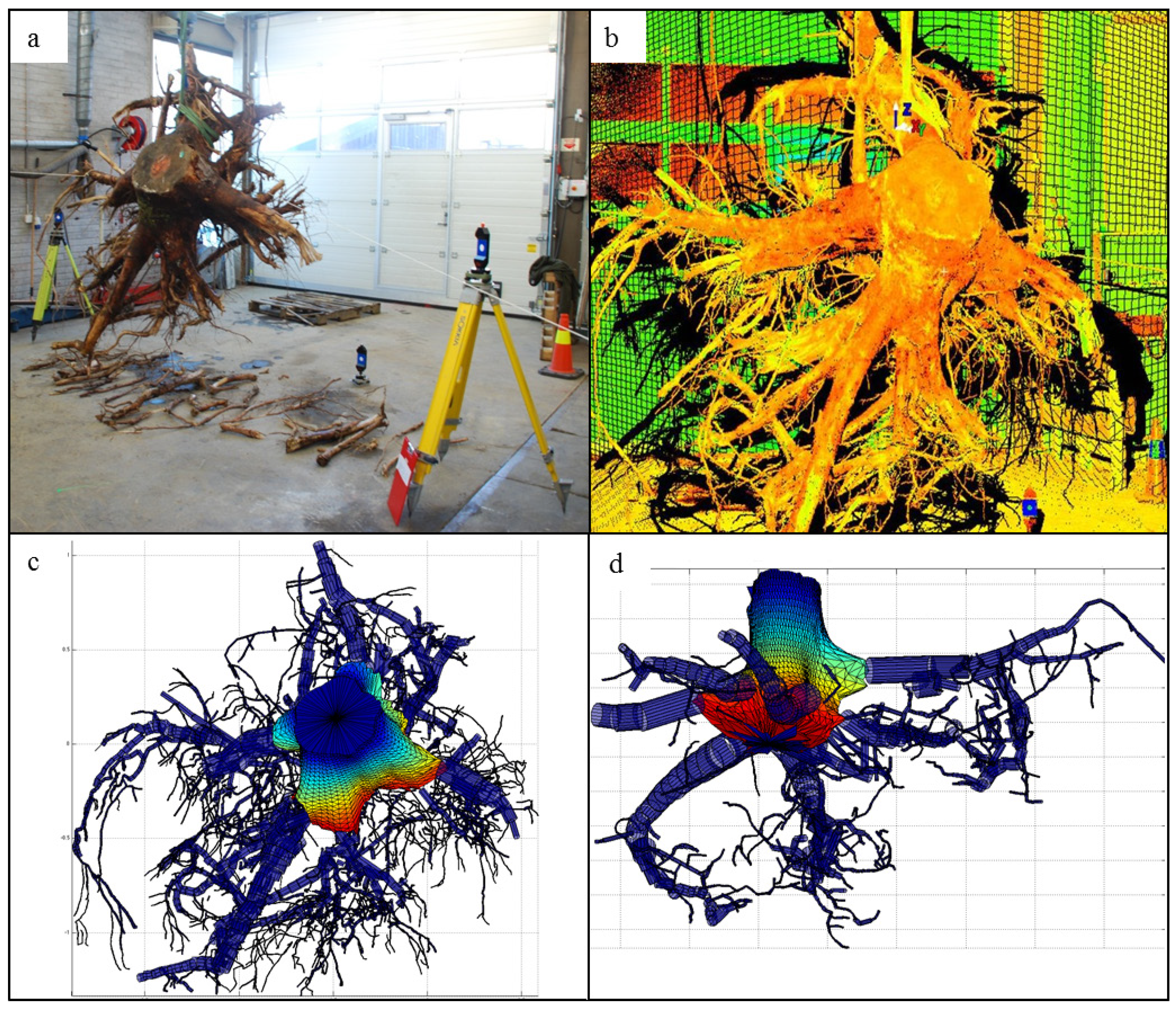
The intact portions of the root systems were completely suspended indoors and individually scanned with a Leica ScanStation 2 terrestrial laser scanner (Leica Geosystems AG, St. Gallen, Switzerland) from three lateral locations located at approximately 120° from each other and within 6 m of the center of each stump (Figure 2a). Any broken root pieces associated with a root system were placed on the floor and included in each scan. Three targets (Leica Geosystems HDS 3” × 3” square Planar Targets, Leica Geosystems AG, St. Gallen, Switzerland) were visible in each scan and used to co-register the scans into a single 3D point cloud of each root system. All scans encompassed the whole root system with a resolution of 2.5 × 2.5 cm at 50 m and a laser beam width of 4 mm (Figure 2b). The co-registered point cloud comprised of all three scans was used to fit the 3D QSM models.

Figure 2. Root system images: (a) Root system 3 suspended at scanning; (b) A 2D reprojection of the TLS point cloud data of root system 3, showing the effects of sensor obscuration (black shadow); (c) Top view of the QSM of root system 3; (d) Oblique bottom view of the QSM of root system 2.

Figure 2. Root system images: (a) Root system 3 suspended at scanning; (b) A 2D reprojection of the TLS point cloud data of root system 3, showing the effects of sensor obscuration (black shadow); (c) Top view of the QSM of root system 3; (d) Oblique bottom view of the QSM of root system 2.

2.4. 3D Quantitative Structure Model (QSM)

2.4.1. Outline of the Method

In this section we give an outline of the basic steps and modeling philosophy behind the method reconstructing the 3D QSMs for the root systems (Figure 2c,d). In the following sections we then describe the steps of the method in detail.

The method is a modified version of the method presented in Raumonen et al. [30] for aboveground tree structures. The idea is to model the surface, volume, and structure of the stump and roots with suitable geometric primitives approximating the local details. The stump portion (bottom part of the primary tree stem) is modeled with a cylindrical triangulation. The root portion (the structures branching out from the stump portion) is modeled as a hierarchical collection of cylinders. The result is a mixed QSM that uses cylindrical triangulation and cylinders as building blocks, which have been selected as the best, simplest, and most robust options for accurately modeling the complex geometry of the root system [41].

The co-registered point cloud is assumed to be a sample of the root system surface. The geometric primitives are used to reconstruct the surface and structure of the root system from the sample. Before the primitives can be fit into the suitable subsets of the point cloud, the stump and root portions need to be separated. Notice that there is no obvious way to define the boundary of the stump and root portions, therefore the stump portion that is modeled with cylindrical triangulation may also contain base portions of the roots that are modeled with cylinders (Figure 2c and Figure 2d). The root portion of the point cloud needs to be further segmented into individual roots, i.e. segments that correspond to a root without any bifurcations.

To realize this separation and segmentation automatically and efficiently, we use a cover set approach, where the point cloud is partitioned into subsets (cover sets) that correspond to small patches along the sampled surface of the root system, similar to the procedure used to segment trees into branches presented in Raumonen et al. [30]. The cover sets (patches) are generated as subsets of randomly but about evenly distributed balls of radius r. The size of the patches is controlled by the user given parameter d which is smaller than r and is (1) the minimum distance between the centers of the balls and (2) the maximum distance between any point and its nearest center. The diameters of the patches vary randomly between d and 2d. The patches are fast to generate, are intuitive to work with, and have a natural neighbor relation and geometric properties facilitating, for example, the easy definition of surface normals. The neighbor relation allows us to easily and naturally expand along the object’s surface and define separate connected components. The details of how to generate covers (a collection of cover sets such that each point in the point cloud belongs to one of the sets), how their neighbor and geometric properties are computed, how to expand along the surface, and how to determine connected components, are explained in Raumonen et al. [30]. In the cases of the stump and roots, we use two different covers; the first has bigger patches for the stump and root separation, and the second has smaller patches for the segmentation of the roots. Covers are also used for filtering noise from the point cloud.

The first major step in the reconstruction method is the filtering of noise from the point cloud. The second step is the separation of the stump and root portions. Modeling the stump portion with a cylindrical triangulation is the third major step. The fourth step is the segmentation of the root portion into individual roots. The final step is the modeling of the roots with cylinders. More details for most these steps and technical features of the reconstruction of QSMs are available in Raumonen et al. [30]. The completed QSMs then allow for the derivation of various root system variables such as: root system volume (total estimated root system volume), diameters (based on cylindrical triangulations for the cut stump surface and cylinder fits for the roots), breakpoint diameters (cylinder diameters of the broken root ends), and linear root length (total summed length of all the cylinders fit to all the roots in the root system). These variables are used to characterize the architecture and volume of the root systems.

2.4.2. Filtering

Co-registered point clouds are first filtered of erroneous points, i.e. points that occupy the empty space near the surface of the object, but that are not part of the sampled surface. These points can cause errors in both the segmentation process and the volume estimates because the modeled points are assumed to represent the surface of the object. Erroneous points are removed by: first, removing low point density areas; and second, removing small separate clusters. In the first case, the point cloud is covered with balls with equal radii and the balls encapsulating less than a pre-defined threshold number of points are removed. In the second case, a new cover with the neighbor relation is generated. The clusters or connected components are then determined, and the clusters that have fewer cover sets than the defined threshold are removed.

The radii and threshold numbers are determined by trial-and-error by making iterative changes in accordance with rapid visual inspections of the filtered point clouds. Radius and threshold values used were 8 mm and six points for the first step and 2 cm and 20 sets in the second. A coordinate point Q was then selected close to the cutting surface of the stump in order to be able to find the surface more reliably later. The rest of the modeling steps are completely automatic.

2.4.3. Separation of the Stump and Roots

After the filtering, the next step is to separate the stump and root portions of the point cloud. The separation of the complex shaped stump surface uses cover sets; we use parameters d = 20 mm (the minimum distance between the centers of the balls and the maximum distance between any point and its nearest center), r = 25 mm (ball radius), and n = 1 (minimum number of points in the ball). The neighbors and the surface normals of the sets were also determined. The separation is based on the idea of looking at the surface from inside the stump. If we go inside the stump along the normal line at the center of the cutting surface of the stump (see Figure 3c), and look into every direction perpendicular to the normal line, then the patches that are closest to the line represent the stump surface. These horizontal search directions are defined by a cylindrical reference consisting of the cutting surface, its normal line at the center, and an arbitrary reference line orthogonal to the normal line. Then the patches are divided into layers (horizontally-oriented slices of the stump portion) and sectors (vertically-oriented slices of the stump portion) according to their height from the cutting surface and azimuth angle from the arbitrary reference line, respectively. The intersection of a layer and a sector then defines a cell in one direction. Selecting suitable patches from each cell then defines the stump portion. A similar idea is used in the cylindrical triangulation model of the stump surface. The points are divided into similar cells except that patches are not selected; instead, the mean of the cell points in each cell defines a vertex of the triangulation.

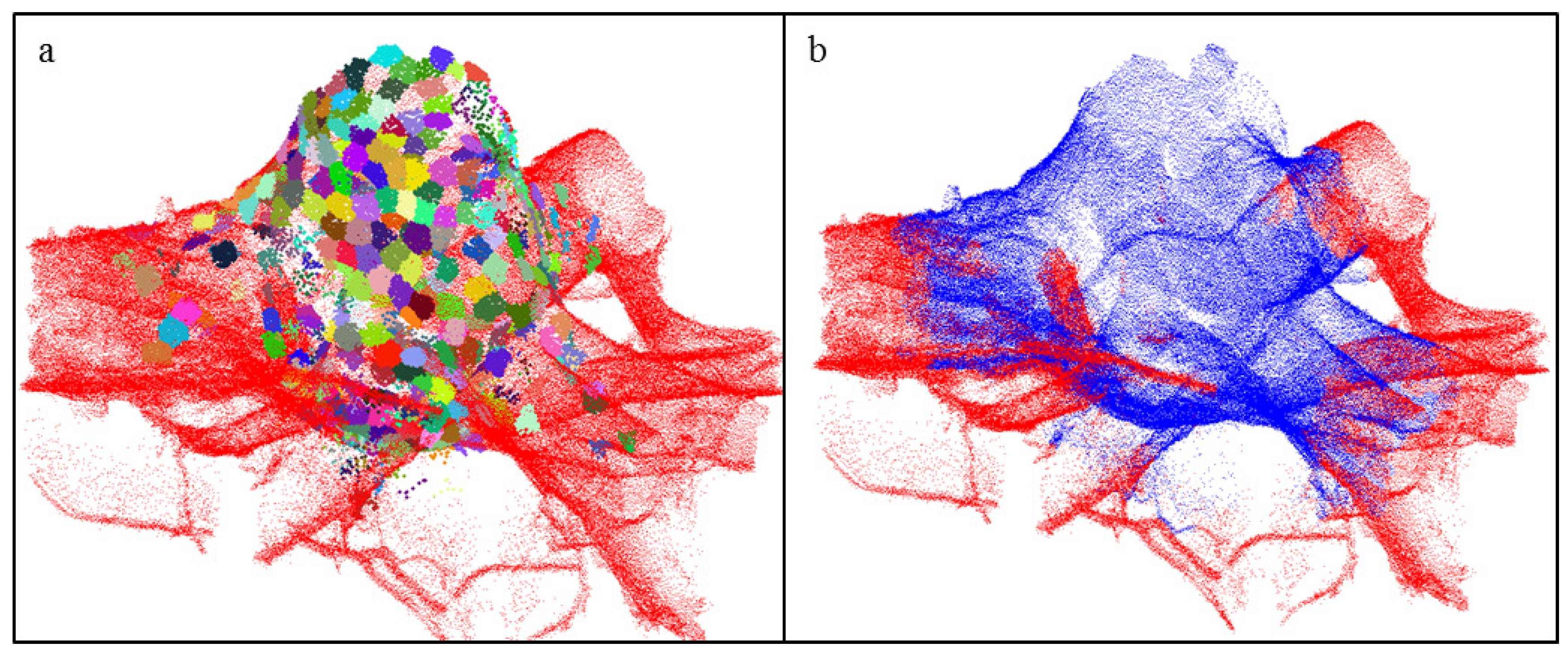
To determine the cutting surface of the stump, the previously determined coordinate point Q on the cutting surface is now used to restrict the cover sets to those closest to Q. These cover sets are then segmented into regions, which are nearly planar (i.e. the angle between normals of the first selected set and other sets of the region does not exceed 10°) and only the largest regions are considered (Figure 3a). The region closest to point Q is then selected as the first approximation for the cutting surface (Figure 3b). A vector is determined that approximates the normal of this region and the region is expanded across neighboring cover sets, but now using a relaxed angle of 20° for normals (Figure 3c).

Figure 3. Determination of the cutting surface: (a) Segmentation of the stump portion into planar regions (only regions with at least five cover sets are shown); (b) Blue points show the initial cutting surface as defined by the selected large region; (c) The final cutting surface (blue) and the normal line (red).

Figure 3. Determination of the cutting surface: (a) Segmentation of the stump portion into planar regions (only regions with at least five cover sets are shown); (b) Blue points show the initial cutting surface as defined by the selected large region; (c) The final cutting surface (blue) and the normal line (red).

The rest of the stump portion is next determined by partitioning the patches into cells by the cylindrical reference defined by the center of the cutting surface, the normal line located there (Figure 3c), and an arbitrary reference line orthogonal to the normal. We only partition patches located in cells that are close to the normal line and located within 3 cm-thick vertically adjacent layers and 12° radial sectors. For each of the cells, the patch that is closest to the normal line is selected (Figure 4a). These patches are then kept or rejected as part of the stump portion with a process carried out for each consecutive layer, which are processed downward starting from the top and ending at the bottom of the stump portion. The bottom is reached when one of the patches in the layer is very close to the normal line. Within each layer, excluding the first layer, a patch is kept if the patch in the above cell is not much closer to the normal line. For example, a patch located along a horizontally extending root surface, which is much further from the normal line than the patch in the above cell, is rejected (Figure 4a). To finalize the stump portion, the selected cover sets are expanded a few times with their neighbors to make the surface complete (Figure 4b).

Figure 4. Determination of the stump portion of the point cloud: (a) Different colors denote the patches closest to the normal line in their cell; (b) The final stump portion is shown in blue.

Figure 4. Determination of the stump portion of the point cloud: (a) Different colors denote the patches closest to the normal line in their cell; (b) The final stump portion is shown in blue.

2.4.4. Modeling the Stump Portion with Cylindrical Triangulation

The separated stump portion of the point cloud is next modeled as a closed triangulation model. The point cloud is partitioned into cells, as in the separation of the stump portion, except we now use 2 cm-thick layers and 5° sectors to get better resolution (Figure 5a). Then the average of the points in each cell forms a vertex of the surface model (Figure 5b). If a cell is empty, the vertex is interpolated between nonempty cells. If vertices occur above and below the empty cell in the same sector, then a linear interpolation between the vertices is used to fill in the missing vertex. If this is not possible, then the missing vertex is interpolated inside the layer between the surface boundary vertices: Let rb and re be the distances of the boundary vertices from the center of the layer, then the distances ri of the n missing vertices are linearly interpolated: ri = rb + i/n × (re − rb). The interpolated vertices are spaced with these distances and equal angles from the center (Figure 5b). All vertices are connected horizontally, vertically, and diagonally to form the triangles of the closed cylindrical triangulation model (Figure 5c). The volumes and diameters for the stump portion can now be easily calculated from this model.

Figure 5. Construction of the closed surface stump model: (a) Stump portion partitioned into cells formed by layers and sectors; (b) Vertices of the triangles from the partition (blue) and interpolation (red); (c) Final closed surface of the cylindrical triangulation model.

Figure 5. Construction of the closed surface stump model: (a) Stump portion partitioned into cells formed by layers and sectors; (b) Vertices of the triangles from the partition (blue) and interpolation (red); (c) Final closed surface of the cylindrical triangulation model.

2.4.5. Segmentation of the Roots

The root portion is next segmented into individual roots using the segmentation process presented in Raumonen et al. [30]. First root bases of the main roots originating from the stump are defined by expanding out from the stump portion (layer B) into patches adjacent to the stump (Figure 6a). Then a new cover with smaller patches (d = 6 mm, r = 8 mm, and n = 5) is defined for the root portion. The cover sets located within layer B determine the connected components of B forming the root bases. In some instances, these components are very small or are edges of the stump and not root bases. These instances are separated out by first sorting the components from the largest to the smallest, and then expanding them about 10 cm each so that each expansion does not extend into previously expanded regions. Components failing to extend enough are rejected. The accepted components form the final bases (see Figure 6b). The next step is to make sure that the rest of the patches covering the root portion are connected to these bases. The connected components of these cover sets are determined and separate components are connected to the nearest component by modifying the neighbor relation of sets accordingly. This process continues as long as all parts of the root portion are connected to some of the root bases.

Figure 6. Determination of bases of the roots originating from the stump: (a) The layer B (red) between the stump (blue) and the rest of the roots (green) forms the bases of the roots; (b) Different colors show the final determined root bases. Notice that some small parts of layer B are not included in the root bases.

Figure 6. Determination of bases of the roots originating from the stump: (a) The layer B (red) between the stump (blue) and the rest of the roots (green) forms the bases of the roots; (b) Different colors show the final determined root bases. Notice that some small parts of layer B are not included in the root bases.

Next the root bases are used as the starting points for the automated root segmentation process described in more detail in Raumonen et al. [30]. Each segment corresponds to a whole or part of a root with no bifurcations. Following the segmentation process, the parent (root stem from which one or more child roots originate and branch from) segments are checked to ensure that their children (roots that originate and branch from the parent root) cannot be combined with the parent root as a continuation of the parent segment. Small child roots, whose maximum distance from the parent root is comparable to the parent’s radius, are removed because it is unclear whether they are part of the parent root. In order to prevent fitting cylinders that are too large at the point of origin of child roots, the child roots are expanded into the parent root and this expansion is removed from both the parent and child roots.

2.4.6. Modeling the Root Portion with Cylinders

The final step is to model the roots with a hierarchical collection of cylinders. Each segment is divided into smaller regions that are then approximated with cylinders using a least squares fitting process [30]. The length of the regions is approximately the user defined parameter l (relative cylinder length = length/radius = 3). After first fitting the regions containing cylinders that are too long, the regions are divided into smaller regions and fit with shorter cylinders in order to force the relative cylinder length to be approximately the given value. The cylinder model is hierarchical in the sense that each cylinder has a root index, order, and parent-child relation. The finished root system QSM consists of the stump portion model with the attached cylindrical root portion model (Figure 2c,d).

3. Results

Visual inspection of the 3D QSM stump models and visualizations of the TLS point cloud data illustrate that the produced models appear to be realistic and complete representations of the coarse root systems (Figure 2).

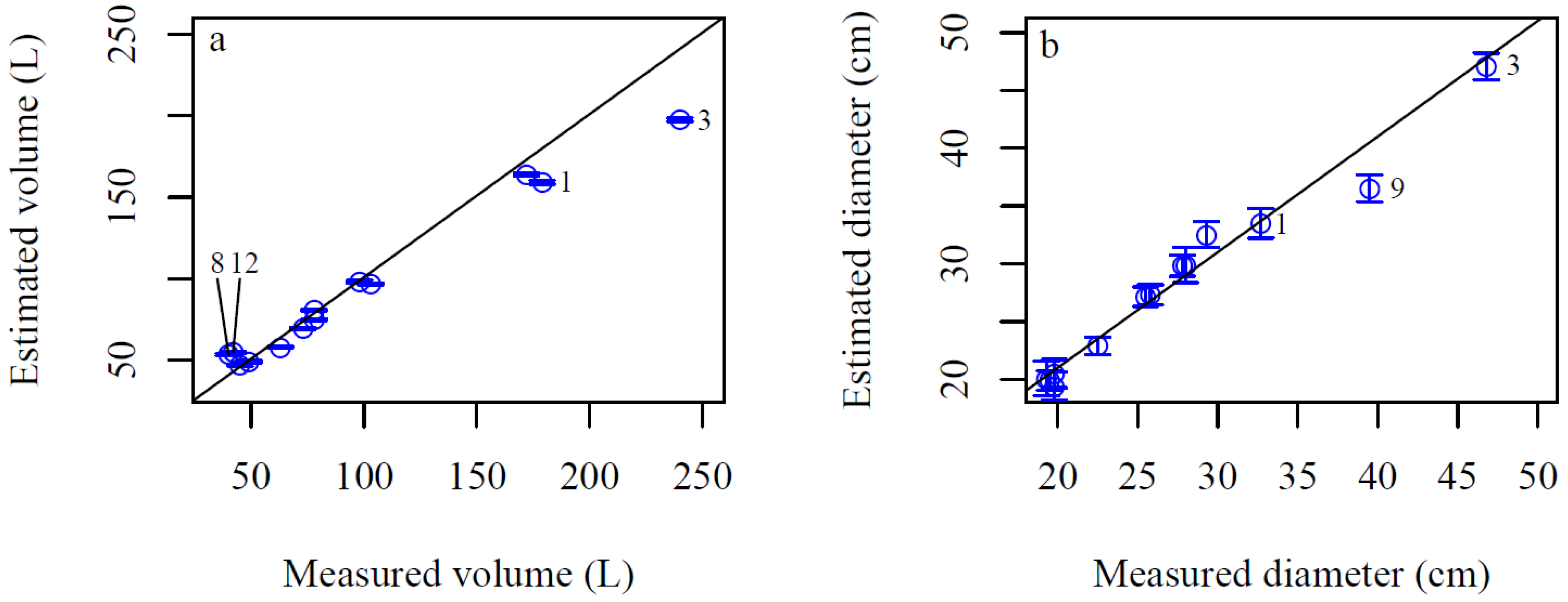
Our results indicate that root system volume can be estimated with relatively high precision using TLS data and the 3D QSMs (Figure 7a). The root system volumes were estimated with a RMSE of 14.4 L (14.9% of the mean measured volume) and a mean prediction error (measured minus predicted values) of 4.3 L (4.4% of the mean measured volume) indicating an underestimation of the volumes (Figure 7a). Overestimates ranged from 0.3 to 34.3% and underestimates from 3.9% to 17.6% of the measured volume. The two largest overestimates were stumps 12 (30.9%) and 8 (34.3%), which where the smallest volume stumps in the study (Figure 7a). The two largest underestimates were stumps 1 (11.1%) and 3 (17.6%), which were the two largest volume stumps in the study (Figure 7a). Most stump diameters estimated from the stump model showed high correlation to the manual measurement (Figure 7b). Stump 9 produced the largest underestimate likely due to a large missing L-shaped section from the stump surface, which was more accurately measured during modeling (Figure 7b). For the diameter estimates, full correlation was not expected as the TLS-based measurements were derived from the average of 27 diameter measurements from the opposite vertices taken from the stump model while the manual measurements were based on two perpendicular diameter measurements.

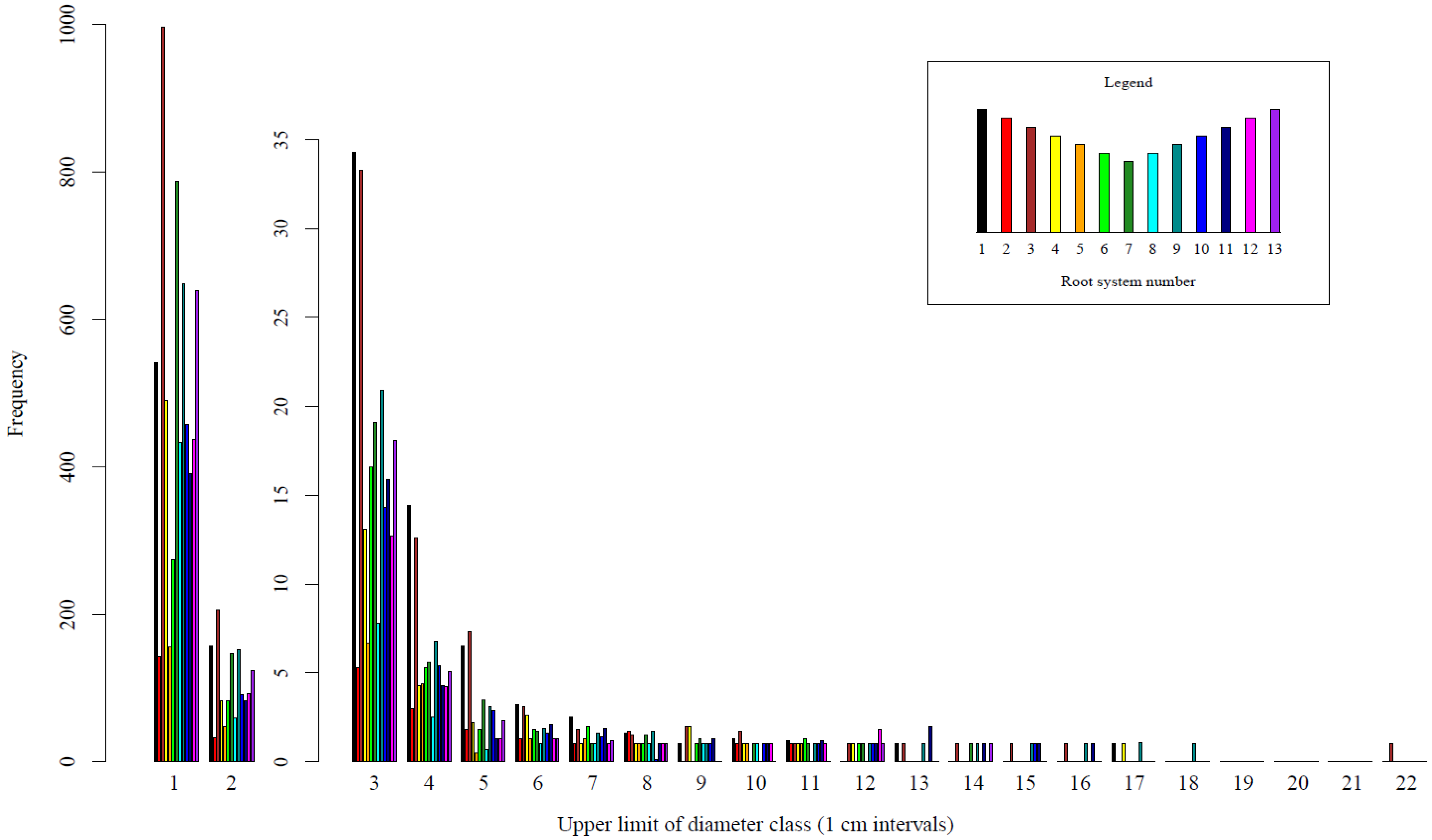
The results illustrate the ability of TLS data, combined with QSM, to estimate important root system architectural and volumetric variables. The root diameter distributions derived from the 3D models illustrate that an average of 55% of the total volume of the root system is comprised of the stump portion (data not shown). On average 16%, 34%, and 43% of the total volume is comprised of roots with a diameter of 5, 10, and 15 cm or less, respectively (data not shown). The frequency of breakpoints in a given diameter class varied between stumps (Figure 8). All stumps had breakpoints less than 8 cm with increasingly more observations in the lower diameter classes (Figure 8). Decreasingly fewer stumps were represented in each of the larger diameter classes by single observations (Figure 8). The largest stump in the study (stump 3; Figure 2a–c) also had the most breakpoints and was represented in all diameter classes up to 16 cm and as large as 21.5 cm (Figure 8). For most of the sampled root systems, the volume of root system left in the soil was likely small in comparison to the extracted root system (Figure 8).

Figure 7. (a) Measured and estimated root system volume and (b) stump diameter. Vertical bars are the standard deviations for the predicted values for 15 model fits for each root system.

Figure 7. (a) Measured and estimated root system volume and (b) stump diameter. Vertical bars are the standard deviations for the predicted values for 15 model fits for each root system.

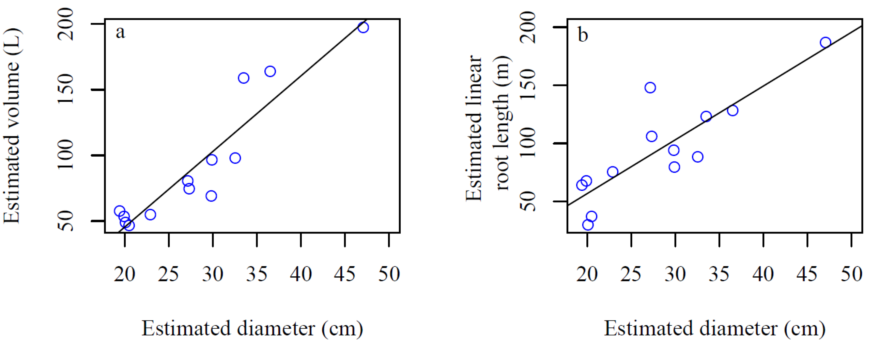
Estimated root system volume and linear root length were found to be correlated to the estimated stump diameter (Figure 9) and simple linear regressions illustrate that stump diameter as the single predictor variable explained 86.8% of the variation in estimated root system volume and 72.1% of the variation in estimated linear root length of the sampled root systems (Figure 9).

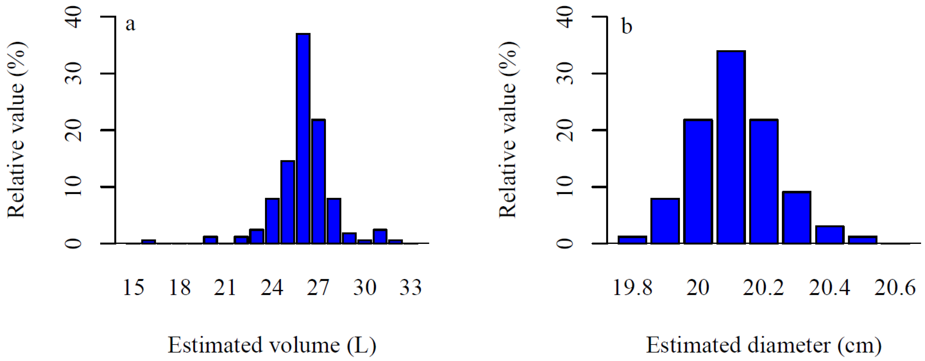
In a sensitivity analysis of the 165 models fitted on the stump portion of root system 2 (Figure 2d), the standard deviation of the volume was 1.85 L or 7% of the average (25.9 L) with about 73% and 90% of the models between 24–28 L and 23–29 L, respectively (Figure 10a). The standard deviation of the stump diameter was 1.3 mm or 0.6% of the average (20.1 cm) (Figure 10b).

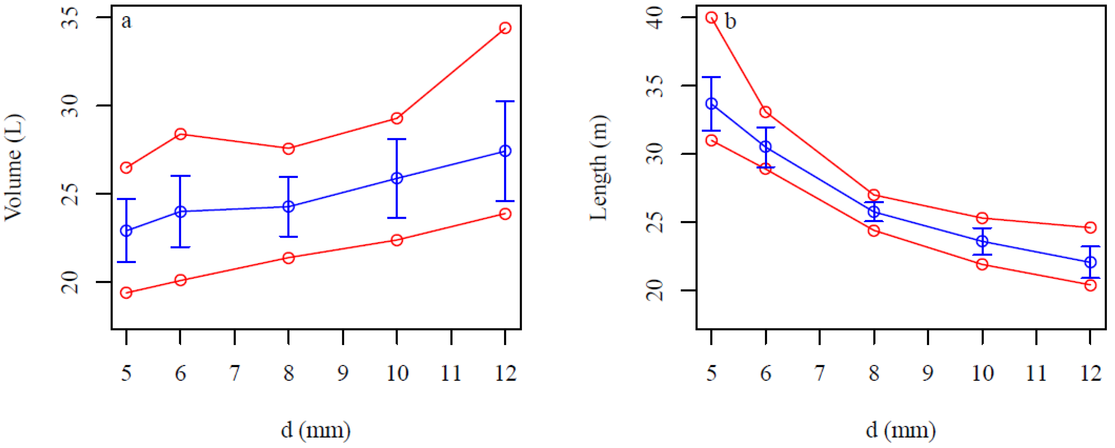
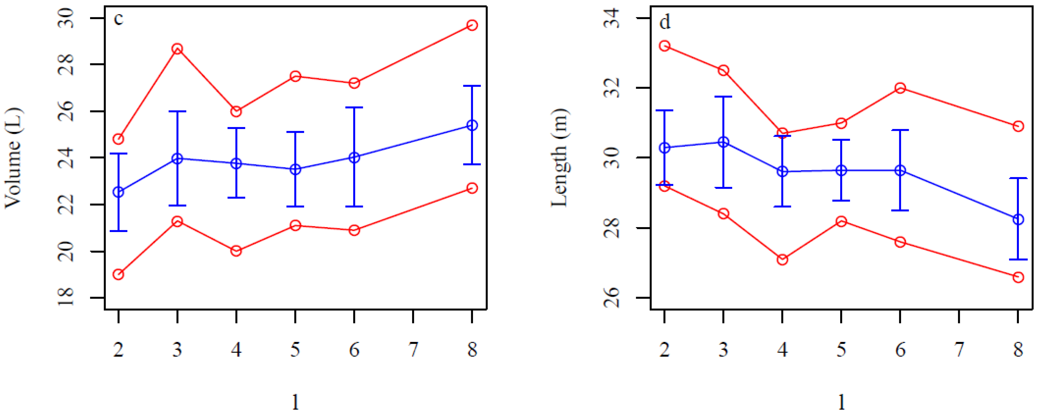
The average root portion volume increased from 22.5 to 27.5 L as d increased with standard deviations of about 7%–10% of the average values (Figure 11a), whereas the average linear root length decreased from 34 to 22 m with standard deviations of about 2.5%–6% (Figure 11b). The average number of roots also decreased from 243 to 98 with increasing values of d (data not shown). The average root portion volume was nearly the same for l values between 2 and 6 with standard deviations of about 6%–9% of the averages (Figure 11c). The average linear root length decreased from 30.5 to 28 m as l increased with standard deviations of about 3%–4% of the averages (Figure 11d).

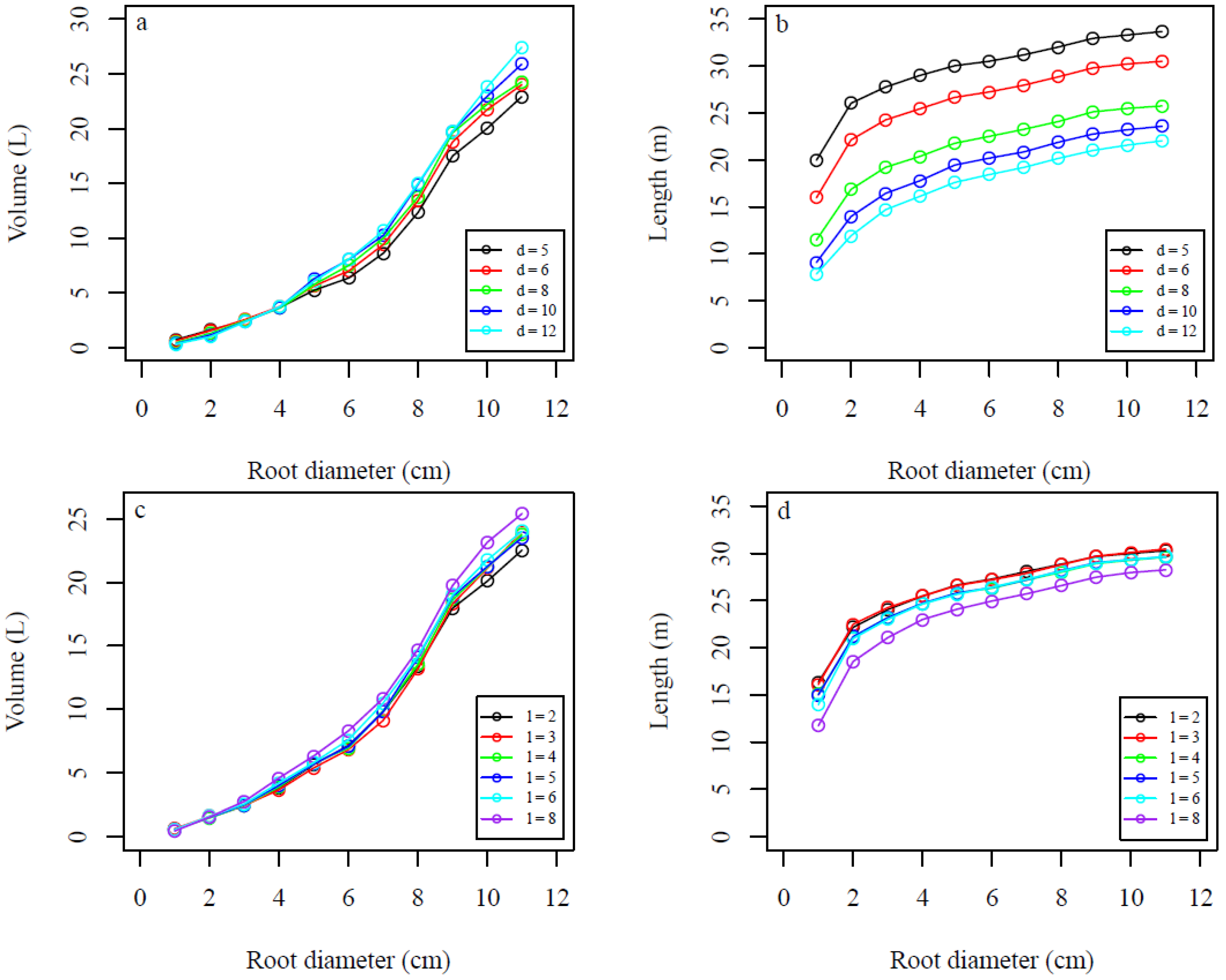
The overall relationships of increasing root volume with increasing values of the d and l parameters (Figure 11a,c, respectively) and decreasing linear root length with increasing values of the d and l parameters (Figure 11b,d, respectively) held as root diameter increased (Figure 12a–d).

Figure 8. Frequency of root breakpoint diameters. Each colored bar represents the mean frequency values in each diameter class for 15 model fits of an individual root system. The same dataset is presented at two different scales to improve legibility within each diameter class.

Figure 8. Frequency of root breakpoint diameters. Each colored bar represents the mean frequency values in each diameter class for 15 model fits of an individual root system. The same dataset is presented at two different scales to improve legibility within each diameter class.

Figure 9. Estimated root system volume and linear root length vs. estimated stump diameter. The lines illustrate fitted regression lines: (a) Root system volume = −69.5563 + 5.7511 × estimated diameter; (b) Linear root length = −35.6380 + 4.6240 × estimated diameter.

Figure 9. Estimated root system volume and linear root length vs. estimated stump diameter. The lines illustrate fitted regression lines: (a) Root system volume = −69.5563 + 5.7511 × estimated diameter; (b) Linear root length = −35.6380 + 4.6240 × estimated diameter.

Figure 10. (a) Distributions of the estimated stump portion volumes (L) and (b) diameters (cm) for 165 model fits of stump 2.

Figure 10. (a) Distributions of the estimated stump portion volumes (L) and (b) diameters (cm) for 165 model fits of stump 2.

Figure 11. Sensitivity of QSMs for the d (the minimum distance between the centers of the balls and the maximum distance between any point and its nearest center) and l (relative cylinder length) parameters for the root portion. (a,c) Total root portion volume and (b,d) linear root length for different (a,b) d values and (c,d) l values. Blue lines are the averages, vertical blue bars are the standard deviations, and red lines are the minimum and maximum values for 15 model fits of stump 2.

Figure 11. Sensitivity of QSMs for the d (the minimum distance between the centers of the balls and the maximum distance between any point and its nearest center) and l (relative cylinder length) parameters for the root portion. (a,c) Total root portion volume and (b,d) linear root length for different (a,b) d values and (c,d) l values. Blue lines are the averages, vertical blue bars are the standard deviations, and red lines are the minimum and maximum values for 15 model fits of stump 2.

Figure 12. Average sensitivity of QSMs for different values of the d (the minimum distance between the centers of the balls and the maximum distance between any point and its nearest center) and l (relative cylinder length) parameters and root diameters for 15 model fits of stump 2. (a,c) Root volume and (b,d) linear root length for different (a,b) d values and (c,d) l values.

Figure 12. Average sensitivity of QSMs for different values of the d (the minimum distance between the centers of the balls and the maximum distance between any point and its nearest center) and l (relative cylinder length) parameters and root diameters for 15 model fits of stump 2. (a,c) Root volume and (b,d) linear root length for different (a,b) d values and (c,d) l values.

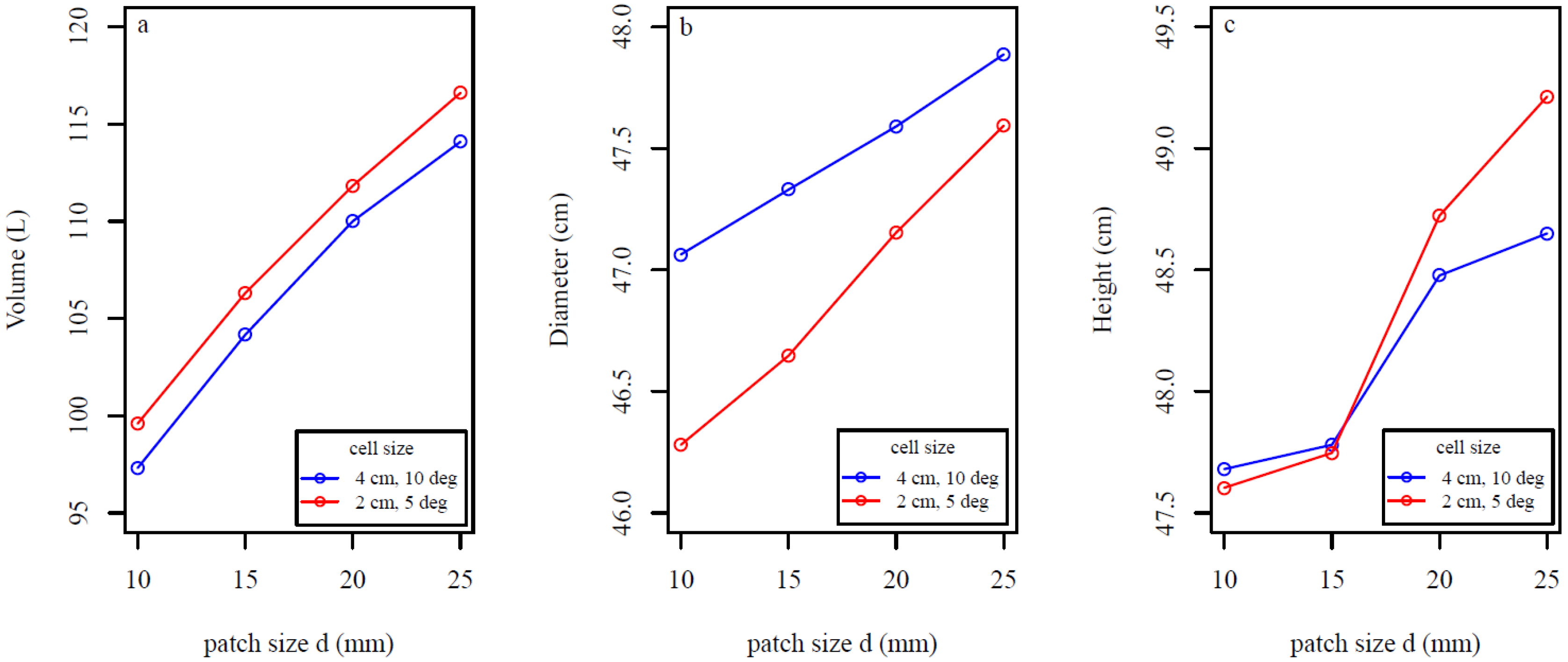
Stump volume, diameter, and height increased with larger cover set patch size d for stump 3 (Figure 13a–c). Stump volume and height increased (Figure 13a,c) with the use of smaller cells, whereas modeled diameter decreased (Figure 13b).

Figure 13. Sensitivity of stump portion (a) volume; (b) diameter; and (c) height to different cover set patch sizes d and cell sizes for 30 model fits of stump 3. Cell size determines the size of the triangles in the cylindrical triangulation model for the stump portion.

Figure 13. Sensitivity of stump portion (a) volume; (b) diameter; and (c) height to different cover set patch sizes d and cell sizes for 30 model fits of stump 3. Cell size determines the size of the triangles in the cylindrical triangulation model for the stump portion.

4. Discussion

Our results indicate that our scanning and stump modeling procedure is capable of rapidly and adequately representing root system architecture and root fraction volumes of multiple large root systems with minimal manual point cloud and modeling post-processing required. Our procedure was able to rapidly describe root variables relevant to the characterization of root volume, such as root diameter, linear root length, break point diameters, number of roots, root fraction counts, and cumulative percentages. Estimated root system volume and estimated linear root length could also be adequately predicted with estimated stump diameter. Taken together, the modeled root system characterizations and volumetric variables provide a highly detailed description of large root systems that can be readily utilized in various applications.

The sensitivity analysis revealed that the standard deviations for estimated stump volume and diameter were in good agreement with the average values (Figure 10). Furthermore, the overall performance of the QSM was shown to be quite stable and predictable against small changes in the d and l parameter values (Figure 10, Figure 11 and Figure 12), as well as changes to the patch sizes (Figure 13). As expected, as d increased root volume increased (Figure 11a and Figure 12a), while linear root length (Figure 11b and Figure 12b) and the average number of roots decreased. This is because smaller cover sets are able to separate smaller roots better and bigger roots more accurately. Also as expected, as l increased root volume increased (Figure 11c and Figure 12c), linear root lengths shortened (Figure 11d and Figure 12d). The linear root lengths shortened because of less accurate curvature approximations. Increasing the patch size d caused the point clouds used for cylindrical triangulation of the stump portion to become larger, increasing modeled stump portion volume and height (Figure 13a,c). Diameter increased because the boundary of the cutting surface became less accurate (Figure 13b). Decreasing the cell size (defining smaller triangles) increased the stump volume and height estimate and decreased the diameter estimate because small curved details are best modeled with smaller triangles. The effect of varying patch and cell size was predictable and relatively small.

The QSM root modeling procedure is capable of describing more topological and volumetric characteristics of whole large root systems than the few examples presented here. Further post-processing of the root models could obtain other root topological and size information previously identified as important by various authors for a wide range of applications [42], such as branching angle, segment length, number of forks, root depth, horizontal spread, root external surface area, and root taper.

The modeling procedures presented here further advance the 3D description of large root systems, best characterizing larger-diameter root architecture. Many of the root measurements that can be made using developed manual analog and digitized measurements can be produced more quickly from TLS point cloud data provided the estimated surfaces are within view of the scanner. Manually digitizing root systems is still superior to TLS in that it is possible to accurately describe all root surfaces regardless of position, but can be much more time consuming. As an example, Danjon and co-workers accurately and completely manually digitized structurally complex large pine trees (mean DBH of 38 cm) to a minimum diameter of 5 mm, taking as many as 10 days per root system [8,21]. In our procedure, each root system was scanned three times within 1.5 h (average 30 min automated scanning and manual scanner set-up each). The point cloud co-registration and post-processing work together with the reconstruction of the QSMs took about 10–20 min per root system. The total scanning and modeling time was about 2 h per root system.

Other scanning methods have been successfully applied to various systems, but each has limitations and presents further challenges. Data acquisition times using CT scanning are very fast and capable of describing root architecture down to <0.5 mm in situ, but so far have only been used to describe root systems of small plants. GPR can describe large coarse root systems in situ under suitable conditions, but reliable accurate reconstructions of root systems in commonly encountered unsuitable conditions are still not possible [25]. Highly accurate (± 50 μm) laser scanning arms have been used to describe a whole root system (pine tree with an 8-cm DBH) down to a diameter of 0.5 mm, but scanning must be done by hand and post-processing times can be demanding with the methodology used by Wagner et al. [37].

Our models underestimated observed root system volume by about 4.4% across all root systems with the overestimates ranging from 0.3% to 34.3% and underestimates ranging from 3.9% to 17.6%. The magnitude of the prediction error is very similar to tree stem QSMs consisting of cylinders (1.36% ± 7.33%) or triangulated meshes (−4.62% ± 2.32%) found by Åkerblom et al. [41]. The exact reasons for the modeled volume underestimate are unclear, but several contributing factors are possible. Occlusion occurs when data for the whole or parts of roots are not captured in the point cloud due to shadowing from the perspective of the scanner. Other studies have shown that the frequency of occlusion can increase with increasing structural root complexity [39] and decreasing number of different scan angles used to generate the point cloud [35]. This study only used three scanning positions per root system and it is likely that any occlusion problems would have been reduced by introducing more scanning positions. However, for most root systems in this study, both structurally simple and complex root systems produced good volume estimates (Figure 7a).

Another contributing factor to the modeled volume underestimate may be that for some root systems, broken root pieces that were separated from but scanned with the root system were not included in the modeled volume estimates. Based on the relatively small size of these pieces for most of the root systems in the study, we do not expect that their inclusion would have drastically reduced the modeled underestimates; however, this could have contributed to the underestimate observed in stumps 1 and 3 (Figure 2a–c; Figure 7a). The reason for the overestimates observed in the small-volume stumps 8 and 12 (Figure 7a) is not clear.

Finally, the question of how well the cylinder model actually fits the roots can be raised. The surface of the root is a reflected sampled surface in TLS point cloud data and is therefore subject to errors related to accuracy of the scanner, reflective properties of the root surface, and the angle of incidence of the laser beam. The modeled cylinder fits of the roots are least squares fits of the sample points closest to the sampled surface and the angle of a longitudinally central vector the length of the defined root segment. In highly crooked root portions, this procedure can yield a proportion of cylinders that are fit incorrectly, that partially overlap, or where “gaps” in portions of roots are not accounted for, leading to an overall underestimate. In other less structurally complex root systems, this same fitting procedure may lead to an overall overestimate.

5. Conclusions

Using TLS to describe and quantify 3D characteristics of whole root systems is in its infancy, but is a promising method that warrants further development. In this study we demonstrate the operational feasibility of applying our root system modeling procedure to 13 mechanically-extracted root systems. Applying our procedure to increasingly larger whole root system data sets would provide new insights into the description of the highly variable belowground structures of plants. Increased topographic and volumetric descriptions of root systems would have important implications for many applications where detailed information on the belowground parts of plants is critical.

References

1. Cairns, M.A.; Brown, S.; Helmer, E.H.; Baumgardner, G.A. Root biomass allocation in the world’s upland forests. Oecologia 1997, 111, 1–11. [Google Scholar] [CrossRef]
2. Kurz, W.A.; Beukema, S.J.; Apps, M.J. Estimation of root biomass and dynamics for the carbon budget model of the Canadian forest sector. Can. J. For. Res. 1996, 26, 1973–1979. [Google Scholar] [CrossRef]
3. Ritson, P.; Sochacki, S. Measurement and prediction of biomass and carbon content of Pinus pinaster trees in farm forestry plantations, south-western Australia. For. Ecol. Manag. 2003, 175, 103–117. [Google Scholar]
4. Bert, D.; Danjon, F. Carbon concentration variations in the roots, stem and crown of mature Pinus pinaster (Ait.). For. Ecol. Manag. 2006, 222, 279–295. [Google Scholar] [CrossRef]
5. Litton, C.M.; Raich, J.W.; Ryan, M.G. Carbon allocation in forest ecosystems. Glob. Chang. Biol. 2007, 13, 2089–2109. [Google Scholar] [CrossRef]
6. Barton, C.V.M.; Montagu, K.D. Effect of spacing and water availability on root: Shoot ratio in Eucalyptus camaldulensis. For. Ecol. Manag. 2006, 221, 52–62. [Google Scholar] [CrossRef]
7. Tobin, B.; Čermák, J.; Chiatante, D.; Danjon, F.; di Iorio, A.; Dupuy, L.; Eshel, A.; Jourdan, C.; Kalliokoski, T.; Laiho, R.; et al. Towards developmental modelling of tree root systems. Plant Biosyst. 2007, 141, 481–501. [Google Scholar] [CrossRef]
8. Danjon, F.; Reubens, B. Assessing and analyzing 3D architecture of woody root systems, a review of methods and applications in tree and soil stability, resource acquisition and allocation. Plat Soil 2008, 303, 1–34. [Google Scholar] [CrossRef]
9. Danjon, F.; Stokes, A.; Bakker, M.R. Root systems of woody plants. In Plant Roots: The Hidden Half, 4th ed.; Eshel, A., Beeckman, T., Eds.; CRC Press: Boca Raton, FL, USA, 2013; pp. 1–26. [Google Scholar]
10. Coates, K.D.; Lilles, E.B.; Astrup, R. Competitive interactions across a soil fertility gradient in a multispecies forest. J. Ecol. 2013, 101, 806–818. [Google Scholar] [CrossRef]
11. Kalliokoski, T.; Nygren, P.; Sievänen, R. Coarse root architecture of three boreal tree species growing in mixed stands. Silva Fenn. 2008, 42, 189–210. [Google Scholar] [CrossRef]
12. Pagès, L.; Vercambre, G.; Drouet, J.L.; Lecompte, F.; Collet, C.; le Bot, J. Root Typ: A generic model to depict and analyse the root system architecture. Plant Soil 2004, 258, 103–119. [Google Scholar] [CrossRef]
13. Godin, C.; Costes, E.; Sinoquet, H. A method for describing plant architecture which integrates topology and geometry. Ann. Bot. 1999, 84, 343–357. [Google Scholar] [CrossRef]
14. Godin, C. Representing and encoding plant architecture: A review. Ann. For. Sci. 2000, 57, 413–438. [Google Scholar] [CrossRef]
15. Nielsen, C.C.N.; Hansen, J.K. Root CSA-root biomass prediction models in six tree species and improvement of models by inclusion of root architectural parameters. Plant Soil 2006, 280, 339–356. [Google Scholar] [CrossRef]
16. Mulatya, J.M.; Wilson, J.; Ong, C.K.; Deans, J.D.; Sprent, J.I. Root architecture of provenances, seedlings and cuttings of Melia volkensii: Implications for crop yield in dryland agroforestry. Agrofor. Syst. 2002, 56, 65–72. [Google Scholar] [CrossRef]
17. Dupuy, L.; Fourcaud, T.; Lac, P.; Stokes, A. A generic 3D finite element model of tree anchorage integrating soil mechanics and real root system architecture. Am. J. Bot. 2007, 94, 1506–1514. [Google Scholar] [CrossRef] [PubMed]
18. Dupuy, L.; Fourcaud, T.; Stokes, A. A numerical investigation into the influence of soil type and root architecture on tree anchorage. Plant Soil 2005, 278, 119–134. [Google Scholar] [CrossRef]
19. Oppelt, A.L.; Kurth, W.; Godbold, D.L. Topology, scaling relations and Leonardo’s rule in root systems from African tree species. Tree Physiol. 2001, 21, 117–128. [Google Scholar] [CrossRef] [PubMed]
20. Danjon, F.; Sinoquet, H.; Godin, C.; Colin, F.; Drexhage, M. Characterisation of structural tree root architecture using 3D digitising and AMAPmod software. Plant Soil 1999, 211, 241–258. [Google Scholar] [CrossRef]
21. Danjon, F.; Fourcaud, T.; Bert, D. Root architecture and wind-firmness of mature Pinus pinaster. New Phytol. 2005, 168, 387–400. [Google Scholar] [CrossRef] [PubMed]
22. Danjon, F.; Bert, D.; Godin, C.; Trichet, P. Structural root architecture of 5-year-old Pinus pinaster measured by 3D digitising and analysed with AMAPmod. Plant Soil 1999, 217, 49–63. [Google Scholar] [CrossRef]
23. Dupuy, L.; Fourcaud, T.; Stokes, A.; Danjon, F. A density-based approach for the modelling of root architecture: Application to Maritime pine (Pinus pinaster Ait.) root systems. J. Theor. Biol. 2005, 236, 323–334. [Google Scholar] [CrossRef] [PubMed]
24. Kaestner, A.; Schneebeli, M.; Graf, F. Visualizing three-dimensional root networks using computed tomography. Geoderma 2006, 136, 459–469. [Google Scholar] [CrossRef]
25. Guo, L.; Chen, J.; Cui, X.; Fan, B.; Lin, H. Application of ground penetrating radar for coarse root detection and quantification: A review. Plant Soil 2013, 362, 1–23. [Google Scholar] [CrossRef]
26. Astrup, R.; Ducey, M.J.; Granhus, A.; Ritter, T.; von Lüpke, N. Approaches for estimating stand-level volume using terrestrial laser scanning in a single-scan mode. Can. J. For. Res. 2014, 44, 666–676. [Google Scholar] [CrossRef]
27. Aschoff, T.; Thies, M.; Spiecker, H. Describing forest stands using terrestrial laser-scanning. Int. Arch. Photogramm. Remote Sens. Spat. Inf. Sci. 2004, 35, 237–241. [Google Scholar]
28. Henning, J.; Radtke, P. Ground-based laser imaging for assessing three-dimensional forest canopy structure. Photogramm. Eng. Remote Sens. 2006, 72, 1349–1358. [Google Scholar] [CrossRef]
29. Hauglin, M.; Astrup, R.; Gobakken, T.; Næsset, E. Estimating single-tree branch biomass of Norway spruce with terrestrial laser scanning using voxel-based and crown dimension features. Scand. J. For. Res. 2013, 28, 456–469. [Google Scholar] [CrossRef]
30. Raumonen, P.; Kaasalainen, M.; Åkerblom, M.; Kaasalainen, S.; Kaartinen, H.; Vastaranta, M.; Holopainen, M.; Disney, M.; Lewis, P. Fast automatic precision tree models from terrestrial laser scanner data. Remote Sens. 2013, 5, 491–520. [Google Scholar] [CrossRef]
31. Bucksch, A.; Fleck, S. Automated detection of branches dimensions in woody skeletons of fruit tree canopies. Photogramm. Eng. Remote Sens. 2011, 77, 229–240. [Google Scholar] [CrossRef]
32. Vonderach, C.; Voegtle, T.; Adler, P. Voxel-based approach for estimating urban tree volume from terrestrial laser scanning data. Int. Arch. Photogramm. Remote Sens. Spat. Inf. Sci. 2012, 39, 451–456. [Google Scholar] [CrossRef]
33. Gärtner, H.; Denier, C. Application of A 3D Laser Scanning Device to Acquire the Structure of Whole Root Systems—A Pilot Study. In Proceedings of the DENDROSYMPOSIUM 2005, Fribourg, Switzerland, 21–23 April 2005; Heinrich, I., Gartner, H., Monbaron, M., Shleser, G., Eds.; TRACE-Tree Rings Archeol, Climatol, and Ecol: Fribourg, Switzerland, 2006; pp. 288–294. [Google Scholar]
34. Teobaldelli, M.; Zenone, T.; Puig, D.; Matteucci, M.; Seufert, G.; Sequeira, V. Structural Tree Modelling of Aboveground and Belowground Poplar Tree Using Direct and Indirect Measurements: Terrestrial Laser Scanning, WGROGRA, AMAPmod and JRC-3D Reconstructor®. In Proceedings of the 5th International Workshop on Functional-Structural Plant Models, Napier, New Zealand, 4–9 November 2007; 2007; pp. 20-1–20-4. [Google Scholar]
35. Gärtner, H.; Wagner, B.; Heinrich, I.; Denier, C. 3D-laser scanning: A new method to analyze coarse tree root systems. For. Snow Landsc. Res. 2009, 82, 95–106. [Google Scholar]
36. Wagner, B.; Gärtner, H.; Ingensand, H.; Santini, S. Incorporating 2D tree-ring data in 3D laser scans of coarse-root systems. Plant Soil 2010, 334, 175–187. [Google Scholar] [CrossRef]
37. Wagner, B.; Santini, S.; Ingensand, H.; Gärtner, H. A tool to model 3D coarse-root development with annual resolution. Plant Soil 2011, 346, 79–96. [Google Scholar] [CrossRef]
38. Wagner, B.; Gärtner, H. 3-D Modeling of Tree Root Systems—A fusion of 3-D laser scans and 2-D tree-ring data. In Proceedings of the RootRAP, International Symposium “Root Research and Applicaitons”, Vienna, Austria, 2–4 September 2009.
39. Wagner, B.; Gärtner, H. Modeling of Tree Roots-Combining 3D Laser Scans and 2D Tree Ring Data. In Proceedings of the DENDROSYMPOSIUM 2008, Zakopane, Poland, 27–30 April 2008; Kaczka, R., Malik, I., Owczarek, P., Gärtner, H., Helle, G., Heinrich, I., Eds.; TRACE-Tree Rings Archeol, Climatol, and Ecol: Zakopane, Poland, 2009; pp. 196–204. [Google Scholar]
40. Liski, J.; Kaasalainen, S.; Raumonen, P.; Akujärvi, A.; Krooks, A.; Repo, A.; Kaasalainen, M. Indirect emissions of forest bioenergy: Detailed modeling of stump-root systems. GCB Bioenerg. 2013. [Google Scholar] [CrossRef]
41. Åkerblom, M.; Raumonen, P.; Kaasalainen, M.; Casella, E. Analysis of geometric primatives in quantitative structure models of tree stems. Remote Sens. 2014, in press. [Google Scholar]
42. Reubens, B.; Poesen, J.; Danjon, F.; Geudens, G.; Muys, B. The role of fine and coarse roots in shallow slope stability and soil erosion control with a focus on root system architecture: A review. Trees 2007, 21, 385–402. [Google Scholar] [CrossRef]