A Stand-Class Growth and Yield Model for Mexico’s Northern Temperate, Mixed and Multiaged Forests

Abstract
:1. Introduction
2. Experimental Section
2.1. Methodology
2.1.1. Fitting, Predicting and Recovering the Weibull Distribution Parameters
2.1.2. The Weibull Density Function
2.1.3. Hypothesis Testing and Goodness-of-Fit
2.1.4. Predicting and Recovering Distribution Parameters

| Model | Stands | Group of Species | Density (No ha−1) | DBH (cm) | S.D (cm) | H (m) | S.D (m) |
|---|---|---|---|---|---|---|---|
| Construction | 587 | Pinus spp. | 631 | 23.4 | 8.7 | 12.6 | 4.5 |
| 587 | Quercus spp. | 212 | 12.8 | 12.8 | 9.3 | 3.2 | |
| Validation | 250 | Pinus spp. | 602 | 23.9 | 8.0 | 11.4 | 4.1 |
| 250 | Quercus spp. | 231 | 12.3 | 11.3 | 9.5 | 3.8 |
2.2. Testing the Independence of the Diameter Distributions of Pines and Oaks
2.3. The Stand-Class Growth and Yield Model
3. Results and Discussion
3.1. Parameter Estimators
| Method | Parameters of the Weibull distribution | |||||||||||
|---|---|---|---|---|---|---|---|---|---|---|---|---|
| α * | β † | ε ‡ | ||||||||||
| Pine | Oak | Pine | Oak | Pine | Oak | |||||||
| A § | SE || | A | SE | A | SE | A | SE | A | SE | A | SE | |
| MNP | 1.6 | 0.0206 | 1.4 | 0.0165 | 26.3 | 0.1403 | 27 | 0.1445 | 12.1 | 0.1114 | 11.1 | 0.1156 |
| MPP | 1.1 | 0.0083 | 0.8 | 0.0124 | 10.8 | 0.1527 | 9.4 | 0.1692 | 14.4 | 0.0495 | 14.5 | 0.0454 |
| MCM | 1.7 | 0.0413 | 1.5 | 0.0454 | 26 | 0.1445 | 25.3 | 0.1527 | 11.7 | 0.2724 | 11.8 | 0.2559 |
| MV2 | 2.0 | 0.0165 | 2.0 | 0.0248 | 28 | 0.1238 | 28.8 | 0.1445 | 13.5 | 0.1238 | 13.8 | 0.1032 |
| MRZ | 1.4 | 0.0165 | 1.1 | 0.0165 | 26.6 | 0.1568 | 27 | 0.2394 | 13.8 | 0.1073 | 14.3 | 0.0949 |
| MDS | 1.8 | 0.0248 | 1.5 | 0.0289 | 15.7 | 0.2311 | 16.9 | 0.3096 | 10.9 | 0.1238 | 10.4 | 0.1445 |
| MRM | 1.6 | 0.0206 | 1.5 | 0.0165 | 13.7 | 0.227 | 15 | 0.227 | 12.3 | 0.1156 | 11.4 | 0.1156 |
| MZM | 1.0 | 0.0083 | 0.8 | 0.0124 | 26.3 | 0.1445 | 26.1 | 0.161 | 14.6 | 0.033 | 14.6 | 0.0413 |
| MV3 | 1.2 | 0.0289 | 0.8 | 0.0289 | 12 | 0.26 | 10.4 | 0.26 | 13.3 | 0.1362 | 14.3 | 0.1568 |
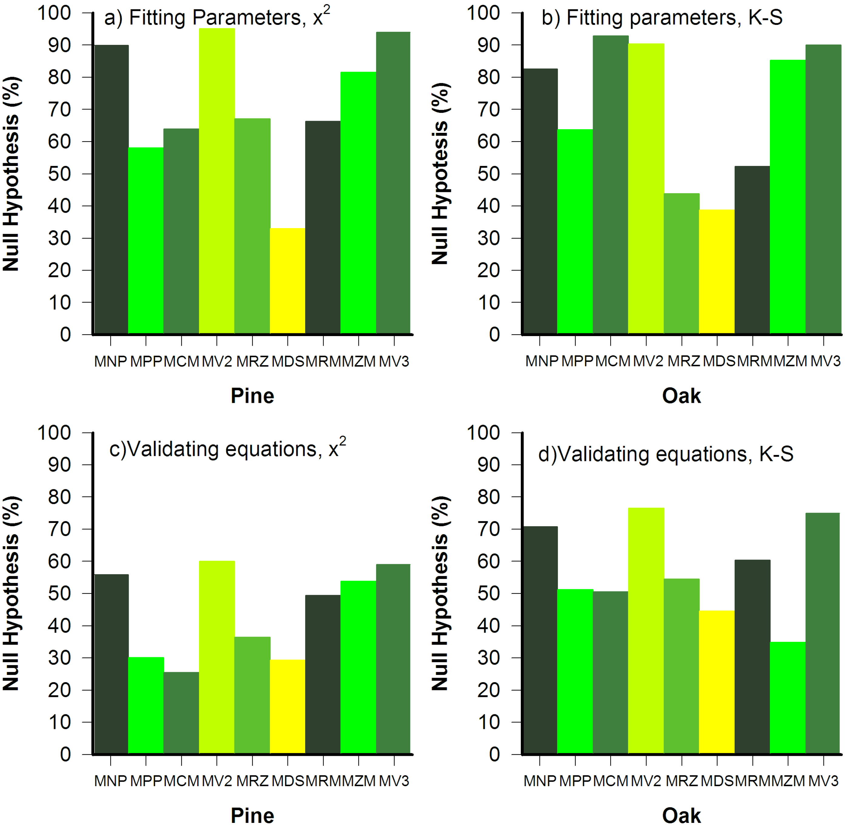
3.2. Goodness of Fit Tests

3.3. Parameter Variance and Bias
| Method | Weibull Distribution Parameters | ||||||||
|---|---|---|---|---|---|---|---|---|---|
| α * | β † | ε ‡ | |||||||
| BP § | A || | S² ¶ | BP | A | S² | BP | A | S² | |
| Pines | |||||||||
| MNP | 0.027 | 1.24 | 0.009 | 0.085 | 25.52 | 0.067 | −0.023 | 13.89 | 0.048 |
| MPP | −0.085 | 1.23 | 0.004 | −0.022 | 11.48 | 0.086 | 0.015 | 14.01 | 0.013 |
| MCM | 0.234 | 1.76 | 0.696 | −1.641 | 25.77 | 14.97 | −4.216 | 11.17 | 40.220 |
| MV2 | 0.035 | 2.86 | 0.001 | −0.053 | 28.23 | 0.084 | ** | 12.50 | ** |
| MRZ | 0.227 | 1.91 | 0.010 | 0.300 | 25.80 | 0.233 | −0.160 | 10.59 | 0.127 |
| MDS | 0.050 | 2.34 | 0.009 | 0.358 | 22.90 | 0.378 | −0.400 | 4.16 | 0.476 |
| MRM | 0.024 | 1.27 | 0.008 | 0.065 | 11.62 | 0.237 | −0.017 | 13.93 | 0.059 |
| MZM | −0.059 | 0.98 | 0.018 | −0.085 | 25.80 | 0.098 | 0.025 | 14.53 | 0.016 |
| MV3 | −0.057 | 1.18 | 0.058 | −0.882 | 12.04 | 13.19 | 0.322 | 13.33 | 1.559 |
| Oaks | |||||||||
| MNP | 0.013 | 0.97 | 0.008 | 0.168 | 25.84 | 0.328 | 0.075 | 13.82 | 0.221 |
| MPP | 0.027 | 0.92 | 0.007 | 0.401 | 11.37 | 0.665 | −0.128 | 14.24 | 0.071 |
| MCM | 1.525 | 2.39 | 5.966 | −1.479 | 26.64 | 18.71 | −9.453 | 5.25 | 27.969 |
| MV2 | −0.006 | 2.17 | 0.007 | 0.088 | 29.50 | 3.497 | ** | 13.00 | ** |
| MRZ | 0.217 | 1.55 | 0.030 | 0.250 | 26.25 | 0.736 | −0.173 | 9.77 | 0.650 |
| MDS | 0.091 | 1.86 | 0.007 | 1.060 | 25.39 | 0.909 | −0.770 | 3.57 | 0.610 |
| MRM | 0.016 | 0.97 | 0.008 | 0.107 | 12.01 | 0.975 | 0.037 | 13.81 | 0.241 |
| MZM | 0.041 | 0.75 | 0.010 | 0.432 | 26.38 | 0.475 | −0.009 | 14.56 | 0.285 |
| MV3 | −0.091 | 0.86 | 0.50 | −0.231 | 10.47 | 31.94 | 0.321 | 14.31 | 10.74 |
3.4. Parameter Prediction and Recovery
| Group of Species | Parameter | Empirical Equation | n | r2 | Sx |
|---|---|---|---|---|---|
| Pinus spp. | α | 0.91Dm13.86Dq−12.31N−0.49BA0.41 | 587 | 0.52 | 0.20 |
| β | 2.9 + 2.2Dm − 0.01N − 1.2Dq + 0.13BA + 0.005Cc + 0.033H | 587 | 0.93 | 0.89 | |
| Xp | 98.5N−0.46BA0.46 | 587 | 0.96 | 0.55 | |
| Std | 1.36 + 0.29Xp − 0.008N + 0.13BA | 587 | 0.68 | 1.10 | |
| Sk | 0.00000021Std2.62N3.14BA−2.93 | 587 | 0.42 | 0.51 | |
| Quercus spp. | α | 0.30β0.99Dm4.18Dq−4.48IDR−0.068 | 587 | 0.51 | 0.21 |
| β | 12.76 + 1.77Dm − 0.035N − 1.13Dq + 0.56BA | 587 | 0.84 | 1.39 | |
| Xp | 92.8N−0.43BA0.43Cc−0.031 | 587 | 0.94 | 0.76 | |
| Std | 799902177Xp−3.5N−2.5BA2.5Cc0.061 | 587 | 0.88 | 1.61 | |
| Sk | 0.00004Std1.9N1.9BA−1.8Cc0.15 | 587 | 0.50 | 0.57 |
3.5. Sensitivity Analysis
| Parameter | Ho Accepted (χ2) | Ho Accepted (K-S) | ||
|---|---|---|---|---|
| Prediction Approach | Pine | Oak | Pine | Oak |
| No change MV2 | 51.3 | 43.7 | 74.7 | 66.7 |
| α ± EES | 32.5 | 36.7 | 71.9 | 65.2 |
| β ± EES | 49.8 | 41.7 | 73.2 | 65.6 |
| α ± EES y β ± EES | 36.2 | 29.1 | 60.2 | 59.2 |
| Predicting Moments Approach | ||||
| No change MNP | 49.8 | 37.5 | 78.4 | 73.7 |
| Sk ± EES | 34.8 | 28.1 | 73.1 | 61.3 |
| Std ± EES | 47.4 | 38.0 | 78.6 | 71.3 |
| Xp ± EES | 48.4 | 38.8 | 81.9 | 70.5 |
| Sk, Std, Xp ± EES | 30.3 | 25.9 | 59.2 | 61.6 |
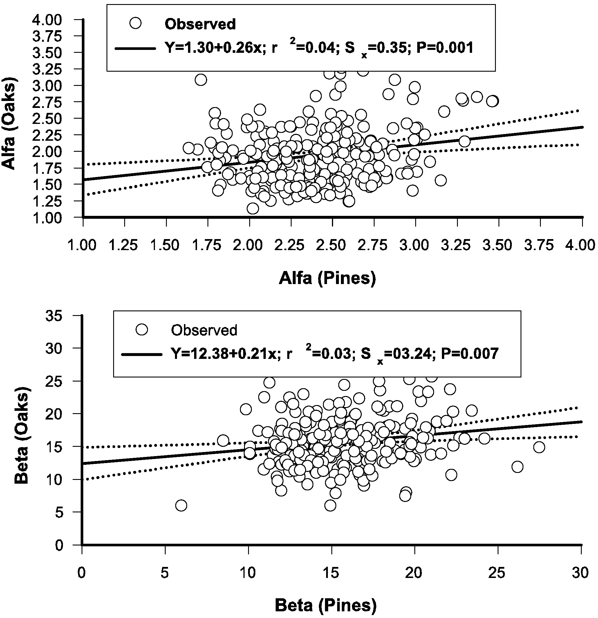
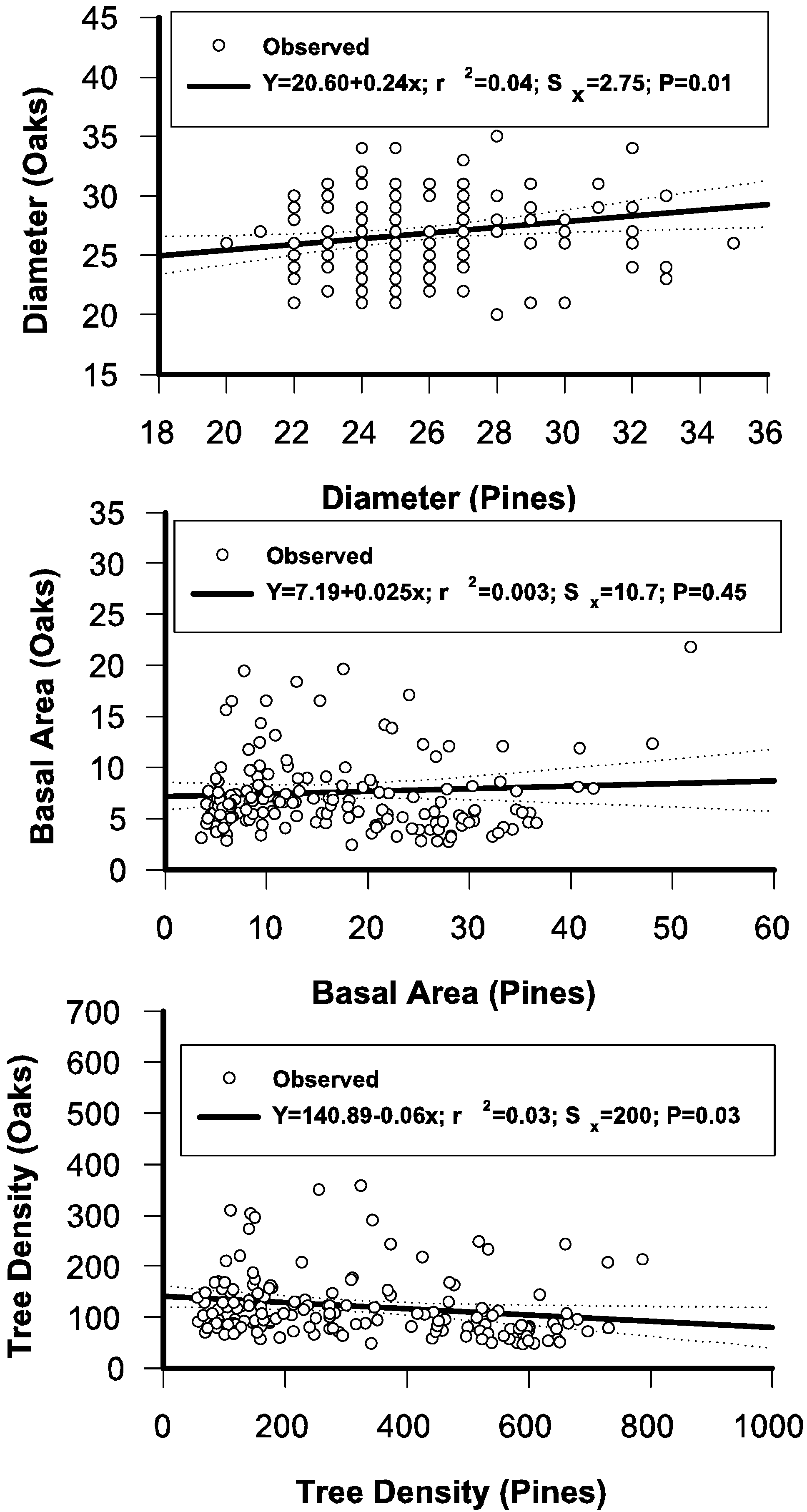
3.6. Regressing Distributional Parameters of Oaks and Pines

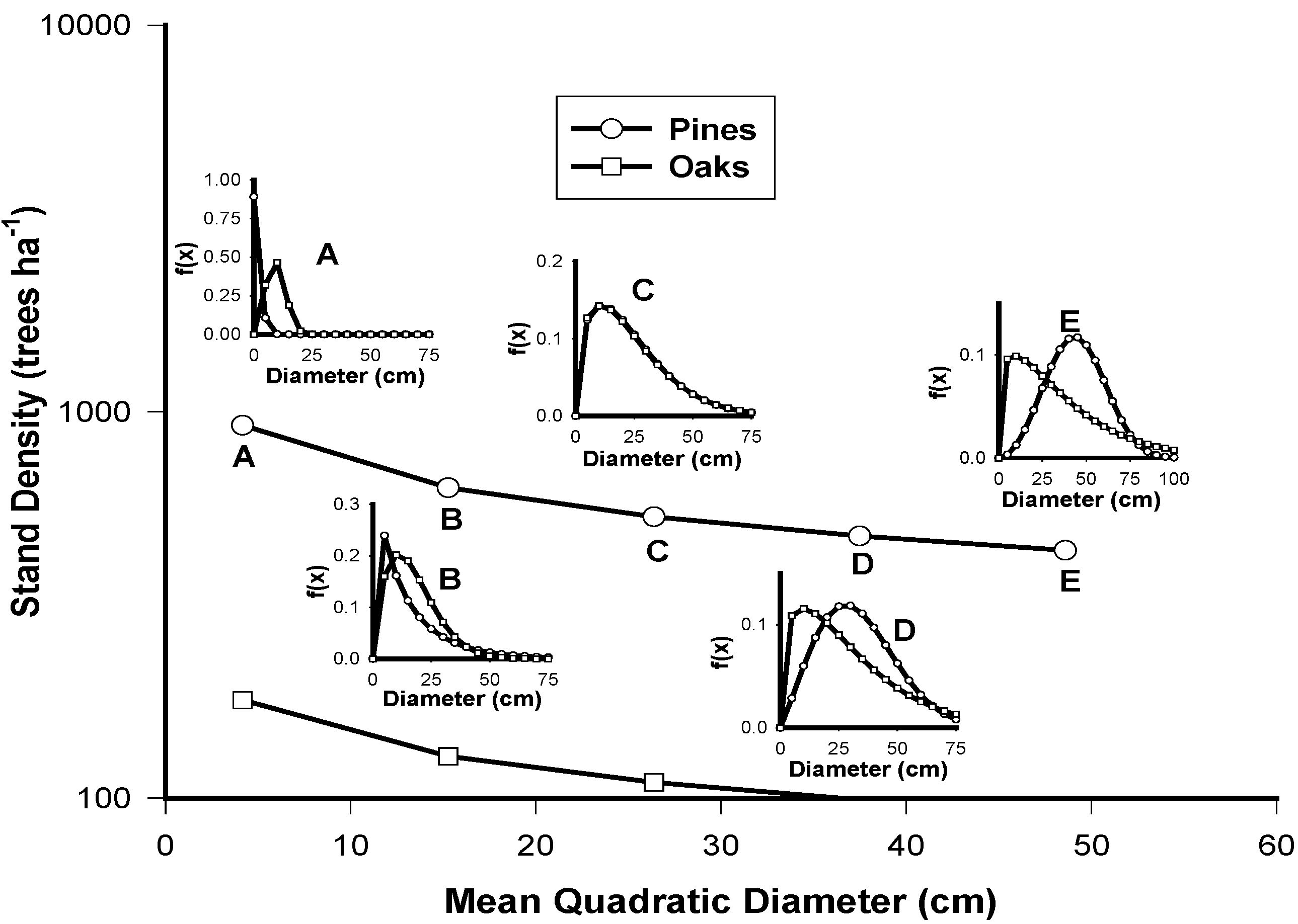
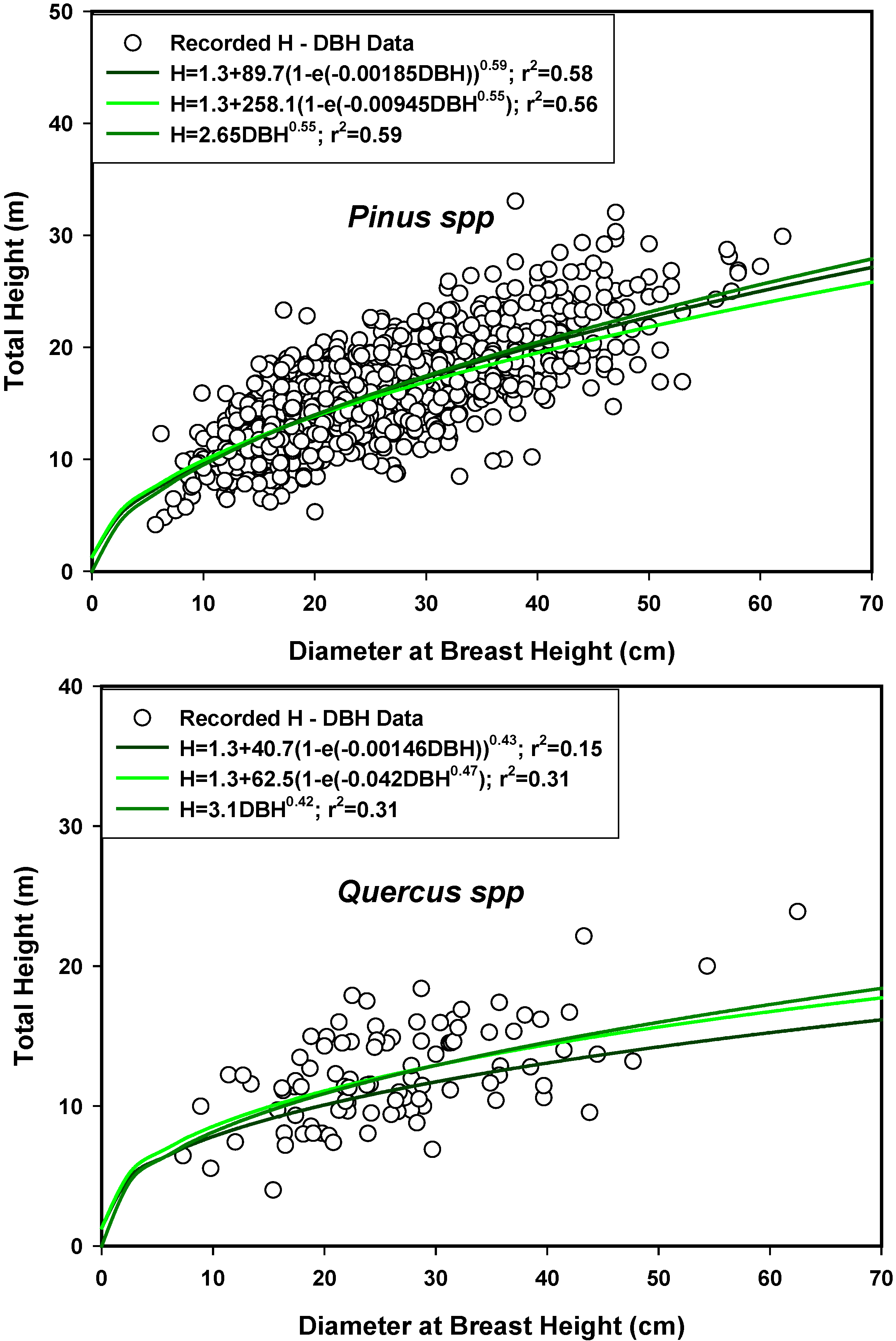
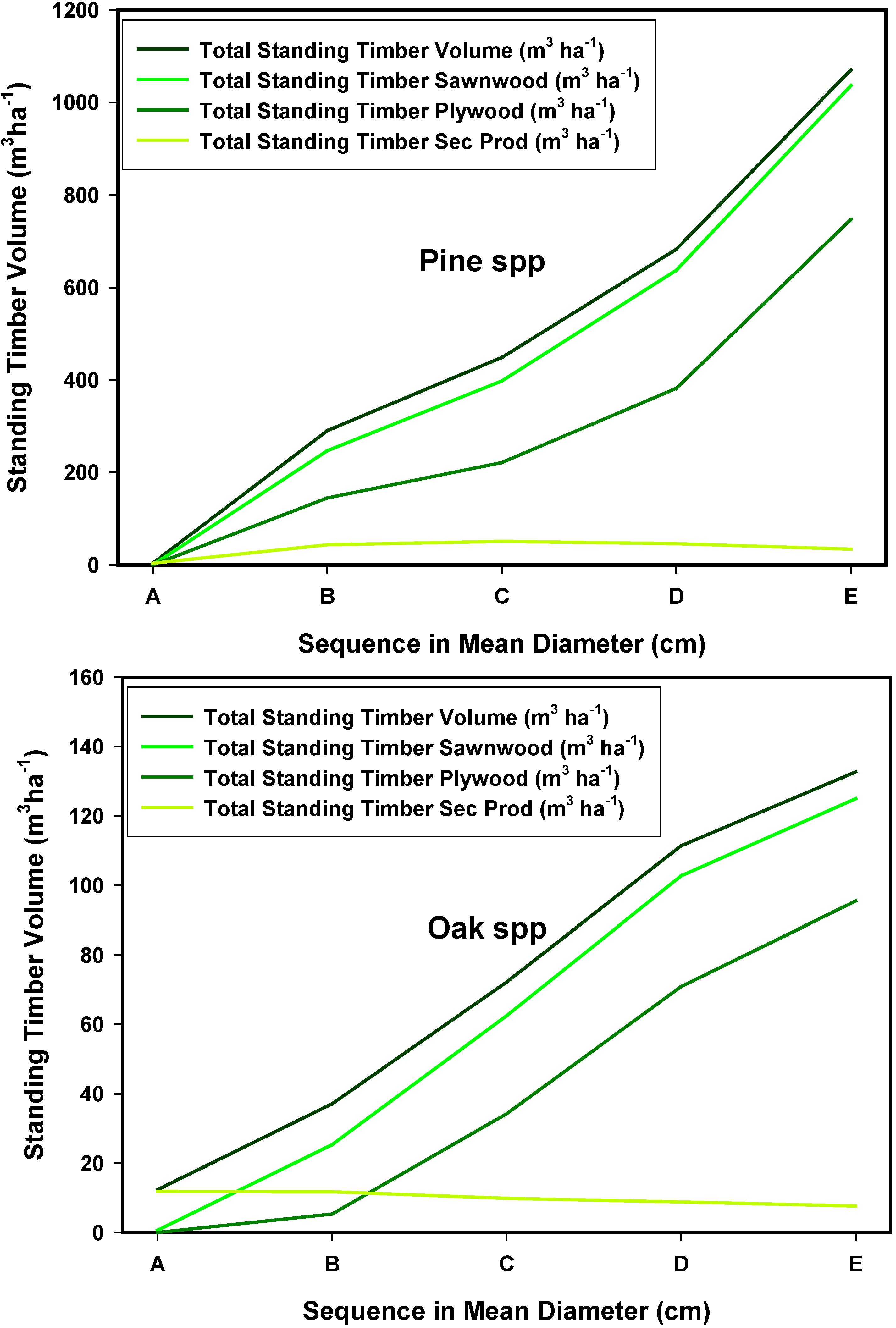
3.7. The Stand-Class Growth and Yield Model

| Attributes/Species | Pinus spp. | Quercus spp. |
|---|---|---|
| Stand Density | 1591.5dmp−0.3392 (r2 = 0.28) | 293.15Dmq−0.3051 (r2 = 0.36) |
| IDR | 30.61Np0.4307 (r2 = 0.65) | 296.9exp0.0007Nq (r2 = 0.43) |
| Dq | 1.1108Dmp−1.3924 (r2 = 0.98) | 0.69Dmq1.1397 (r2 = 0.99) |
| H | 1.5158Dmp0.7217 (r2 = 0.47) | 0.9054Dmq0.8499 (r2 = 0.55) |
| Cc | 69.403Dmp−0.1429 (r2 = 0.87) | 2.29Dmq0.8626 (r2 = 0.56) |


4. Conclusions
Conflicts of Interest
References
- Food and Agriculture Organization (FAO), UN. State of the World Forests; Forestry Department: Rome, Italy, 2012. Available online: www.fao.org (accessed on 14 August 2014).
- Food and Agriculture Organization (FAO), UN. Global Forest Resource Assessments 2010; Forestry Department: Rome, Italy, 2010. Available online: www.fao.org (accessed on 15 August 2014).
- Vanclay, K.V. Modeling Forest Growth and Yield: Applications to Mixed Tropical Forests; CAB International: Wallingford, Oxon, UK, 1994; p. 312. [Google Scholar]
- Vanclay, J.K. Growth models for tropical forest: A synthesis of models and methods. For. Sci. 1995, 41, 7–42. [Google Scholar]
- Návar-Cháidez, J.; González-Elizondo, M.S. Diversidad, estructura y productividad de los bosques templados de Durango, México. Polibotanica 2009, 27, 71–87. [Google Scholar]
- Capri, C.A. Silvicultura Intensiva en Bosques Templados de México; División de Ciencias Forestales, Universidad Autónoma Chapingo: Texcoco, México, 1990. [Google Scholar]
- Aguirre-Bravo, C. Stand average and Diameter Distribution Growth and Yield Models for Natural Even-Aged Stands of Pinus cooperii. Ph.D. Thesis, Colorado State University, Fort Collins, CO, USA, 4 September 1987; p. 147. [Google Scholar]
- Zepeda, B.M.; Acosta, E.M. Incremento y rendimiento maderable de Pinus montezumae Lamb., en San Juan Tetla, Puebla. Madera Bosques 2000, 6, 15–27. [Google Scholar]
- Luna, G.; de Jesús, J. Técnicas de evaluación dasométrica y ecológica de los bosques de coníferas bajo manejo de la Sierra Madre Occidental del centro sur de Durango, México. Master Thesis, Universidad Autónoma de Nuevo León, Linares, NL, México, 2001. [Google Scholar]
- Ishi, H.T.; Tanabe, S.; Hiura, T. Exploring the relationship among canopy structure, stand productivity, and biodiversity of temperate forest ecosystems. For. Sci. 2004, 50, 342–355. [Google Scholar]
- Vilá, M.; Vayreda, J.; Comas, L.; Ibañez, J.J.; Mata, T.; Obón, B. Species richness and Wood production: A positive association in Mediterranean forests. Ecol. Lett. 2007, 10, 241–250. [Google Scholar] [CrossRef] [PubMed]
- Juárez, M.; Domínguez-Calleros, P.A.; Návar-Cháidez, J.J. Análisis de la estructura silvícola en bosques de la Sierra de San Carlos, Tamaulipas, Mexico. For. Veracruz. 2014, 16, 25–34. [Google Scholar]
- Stevens, M.H.H.; Carson, W.P. Plant density determines species richness along an experimental fertility gradient. Ecology 1999, 80, 455–465. [Google Scholar] [CrossRef]
- Hooper, D.U.; Vitousek, P.M. The effect of plant composition and diversity on ecosystem processes. Science 1997, 277, 1302–1305. [Google Scholar] [CrossRef]
- Peng, C.H. Growth and yield models for uneven-aged stands: Past present and future. For. Ecol. Manag. 2000, 132, 259–279. [Google Scholar] [CrossRef]
- Clutter, J.L.; Fortson, J.C.; Pienaar, L.V.; Brister, G.H.; Bailey, R.L. Timber Management: A Quantitative Approach; John Wiley and Sons: New York, NY, USA, 1983; pp. 3–29. [Google Scholar]
- Botkin, D.B.; Janak, J.F.; Wallis, J.R. Some ecological consequences of a computer model of forest growth. J. Ecol. 1972, 60, 849–872. [Google Scholar] [CrossRef]
- Moser, J.W. Specification of density for inverse j-shaped diameter distribution. For. Sci. 1976, 22, 177–180. [Google Scholar]
- Shugart, H.H. A Theory of Forest Dynamics; Springer Verlag: New York, NY, USA, 1984. [Google Scholar]
- Bailey, R.L.; Dell, T.R. Quantifying diameter distributions with the Weibull function. For. Sci. 1973, 19, 97–104. [Google Scholar]
- Zhou, B.; McTague, P.G. Comparison and evaluation of five methods of estimation of the Johnson systems parameters. Can. J. For. Res. 1996, 26, 928–935. [Google Scholar] [CrossRef]
- Cao, Q.V. Predicting parameters of a Weibull function for modeling diameter distribution. For. Sci. 2004, 50, 682–685. [Google Scholar]
- Parresol, B.; Fonseca, T.F.; Marques, C.P. Numerical Details and SAS Programs for Parameter Recovery of the SB Distribution; General Technical Report SRS-122; Asheville, N.C., Ed.; USA Department of Agriculture Forest Service, Southern Research Station: Asheville, NC, USA, 2010; p. 27. [Google Scholar]
- Haan, C.T. Statistical Methods in Hydrology; Iowa State Press: Ames, IA, USA, 2003; p. 378. [Google Scholar]
- Wingo, D.R. Maximum likelihood estimation of the parameters of the Weibull distribution by modified quasilinearization. IEEE Trans. Reliab. 1972, 2, 89–93. [Google Scholar] [CrossRef]
- Návar-Cháidez, J.J.; Contreras-Aviña, J. Ajuste de la distribución Weibull a las estructuras diametricas de rodales irregulares de pino de Durango, México. Agrociencia 2000, 34, 356–361. [Google Scholar]
- Parresol, B. Recovering parameters of Johnson’s SB distribution: A demonstration with loblolly pine. Can. J. For. Res. 2001, 31, 865–878. [Google Scholar] [CrossRef]
- Torres-Rojo, J.M. Predicción de distribuciones diamétricas multimodales a través de mezclas de distribuciones Weibull. Agrociencia 2005, 39, 211–220. [Google Scholar]
- Burke, T.E.; Newberry, J.D. A simple algorithm for moment based recovery of Weibull distribution parameters. For. Sci. 1984, 30, 329–332. [Google Scholar]
- Shiver, B.D. Sample size and estimation methods for the Weibull distribution for unthinned slash pine plantation diameter distributions. For. Sci. 1988, 34, 809–814. [Google Scholar]
- Lindsay, S.R.; Wood, G.R.; Woollons, R.C. Stand table modeling through the Weibull distribution and usage of skewness information. For. Ecol. Manag. 1996, 81, 19–23. [Google Scholar] [CrossRef]
- Zanakis, S.H. A simulation study of some simple estimators for the three parameter Weibull distribution. J. Stat. Comput. Simul. 1979, 9, 101–116. [Google Scholar] [CrossRef]
- Hyink, D.M.; Moser, J.W., Jr. A generalized framework for projecting forest yield and stand structure using diameter distributions. For Sci. 1983, 29, 85–95. [Google Scholar]
- Hynk, D.M. Diameter distribution approaches to growth and yield modeling. In Forecasting Forest Stand Dynamics; Brown, K.M., Clarke, F.R., Eds.; Lakehead University: Thunderbay, Ontario, Canada, 1980; pp. 138–163. [Google Scholar]
- Da Silva, J.A.A. Dynamics of Stand Structure in Fertilized Slash Pine Plantations. Ph.D. Thesis, University of Georgia, Athens, GA, USA, 1986; p. 139. [Google Scholar]
- Devore, J.L. Probability and Statistics for Engineers and the Sciences; Brooks/Cole Publishing Company: San Luis Obispo, CA, USA, 1987; p. 312. [Google Scholar]
- Návar-Cháidez, J.J. Estimaciones empíricas de parámetros de la distribución Weibull en bosques nativos del norte de México. Rev. For. Latinoam. 2009, 24, 51–68. [Google Scholar]
- Návar, J.; Jiménez, J.; Domínguez, P.A.; Aguirre, O.A.; Galvan, M.; Paez, M.A. Predicción del crecimiento de masas forestales irregulares en base a las distribuciones dimétricas en el sureste de Sinaloa, México. Investig. Agraría. Sis. Rec. For. 1996, 5, 214–229. [Google Scholar]
- Palahi, M.; Pukkala, T.; Trasobares, A. Modeling the diameter distribution of Pinus sylvestris, Pinus nigra and Pinus halepensis forest stands in Catalonia using the truncated Weibull function. Forestry 2006, 79, 553–562. [Google Scholar] [CrossRef]
- Corral-Rivas, S.; Návar-Cháidez, J.J. Comparación de técnicas de estimación de volumen fustal total para cinco especies de pino de Durango, México. RCHSCFA 2013, 15, 5–13. [Google Scholar]
- Merlin-Bermúdez, E.; Návar-Cháidez, J.J. Desarrollo de modelo de incremento y rendimiento para Quercus sideroxylla en bosques mixtos de Durango, México. Agrofaz 2005, 5, 875–882. [Google Scholar]
- Návar, J.J.; Rodríguez-Flores, F.J.; Domínguez-Calleros, P.A. Taper functions and merchantable timber for temperate forests of Northern Mexico. Ann. For. Res. 2013, 56, 165–178. [Google Scholar]
- Newnham, R.M. Variable-form taper functions for four Alberta trees. Can. J. For. Res. 1992, 22, 201–223. [Google Scholar] [CrossRef]
- Borders, B.E.; Patterson, T.W. Projecting stand tables—A comparison of the Weibull diameter distribution method, a percentile-based projection method, and a basal area growth projection method. For. Sci. 1992, 36, 413–424. [Google Scholar]
- Cao, Q.V.; Baldwin, V.C. A new algorithm for stand table projection models. For. Sci. 1999, 45, 506–511. [Google Scholar]
- Kangas, M.M.A.; Utera, J.; Tornianien, T.; Saramaki, J. Comparison of percentile based prediction methods and the Weibull distribution in describing the diameter distribution of heterogeneous Scots pine stands. For. Ecol. Manag. 2000, 133, 263–274. [Google Scholar] [CrossRef]
- Návar-Cháidez, J.J.; Domínguez-Calleros, P.A. Modelos de incremento y rendimiento: Ejemplos y aplicaciones para bisques templados Mexicanos. Rev. Mex. Cienc. For. 2013, 4, 8–26. [Google Scholar]
- Navarro-Cerrillo, R.; Manzanedo, R.; Bohorque, J.; Sánchez, J.; de Miguel, S.; Solano, D.; Qarro, M.; Griffith, D.; Palacios, G. Structure and spatio-temporal dynamics of cedar forests along a management gradient in Middle Atlas, Morocco. For. Ecol. Manag. 2013, 289, 341–353. [Google Scholar] [CrossRef]
- Laar, A.V.; Mosandl, R.; van Laar, A. Diameter distributions in young oak stands. Allg. For. Jagdzeitg. 1989, 160, 189–194. [Google Scholar]
- Nanang, D.M. Suitability of the normal, log-normal and Weibull distributions for fitting diameter distributions for neem plantations in northern Gahana. For. Ecol. Manag. 1998, 103, 1–7. [Google Scholar] [CrossRef]
- Knowe, S.A.; Harrington, T.B.; Shula, R.G. Incorporating the effects of interspecific competition and vegetation management treatments in diameter distribution models for Douglas fir saplings. Can. J. For. Res. 1992, 22, 1255–1262. [Google Scholar] [CrossRef]
- Newberry, J.D.; Moore, J.; Zhang, J.L.; Zhang, L. Evaluation of simple quantile estimation functions for modeling forest diameter distribution in even-aged stands of interior Douglas-fir. Can. J. For. Res. 1993, 23, 2376–2382. [Google Scholar] [CrossRef]
- Gove, J.H.; Patil, G.P. Modeling the basal area-size distribution of forest stands: A compatible approach. For. Sci. 1998, 44, 285–297. [Google Scholar]
- Márquez-Linares, M.A.; Alvarez-Zagoya, R. Construcción de una guía de densidad para Pinus cooperi var. Ornelasi con base en la clase de copa en Durango, Mexico. Madera y Bosques 1995, 1, 23–36. [Google Scholar]
- Callaway, R.M.; Walker, L.R. Competition and facilitation: A synthetic approach to interactions in plant communities. Ecology 1997, 78, 1958–1965. [Google Scholar] [CrossRef]
- Callaway, R.M. Competition and facilitation on elevation gradients in subalpine forests of the northern Rocky Mountains, USA. Oikos 1998, 82, 561–573. [Google Scholar] [CrossRef]
- Lafon, C.W.; Houston, M.A.; Horn, S.P. Effects of agricultural soil loss on forest succession rates and tree diversity in east Tennessee. Oikos 2000, 90, 431–441. [Google Scholar] [CrossRef]
- De Los Ríos, C.E. Facultad de Ciencias Forestales. Ph.D. Thesis, Universidad Nacional de Santiago del Estero, Linares, NL, México, 2001. [Google Scholar]
- Domínguez, P.A.; Návar, J. I Congreso Mexicano de Recursos Forestales; Sociedad Mexicana de Recursos Forestales: Saltillo, Coahuila, México, 1993. [Google Scholar]
- Návar, J.; Estrada, C.; Contreras, J.C.; Domínguez, P.A.; Muller-Using, B. Evaluation of the abundance, form of establishment, and the causes of variation of pine regeneration in coniferous stands of the western Sierra Madre of Durango, Mexico. Forstarchiv 2001, 72, 175–179. [Google Scholar]
© 2014 by the authors; licensee MDPI, Basel, Switzerland. This article is an open access article distributed under the terms and conditions of the Creative Commons Attribution license (http://creativecommons.org/licenses/by/4.0/).
Share and Cite
Návar, J. A Stand-Class Growth and Yield Model for Mexico’s Northern Temperate, Mixed and Multiaged Forests. Forests 2014, 5, 3048-3069. https://doi.org/10.3390/f5123048
Návar J. A Stand-Class Growth and Yield Model for Mexico’s Northern Temperate, Mixed and Multiaged Forests. Forests. 2014; 5(12):3048-3069. https://doi.org/10.3390/f5123048
Chicago/Turabian StyleNávar, José. 2014. "A Stand-Class Growth and Yield Model for Mexico’s Northern Temperate, Mixed and Multiaged Forests" Forests 5, no. 12: 3048-3069. https://doi.org/10.3390/f5123048
APA StyleNávar, J. (2014). A Stand-Class Growth and Yield Model for Mexico’s Northern Temperate, Mixed and Multiaged Forests. Forests, 5(12), 3048-3069. https://doi.org/10.3390/f5123048