Spatial Characterization of Wildfire Orientation Patterns in California


Abstract
:1. Introduction
2. Methods
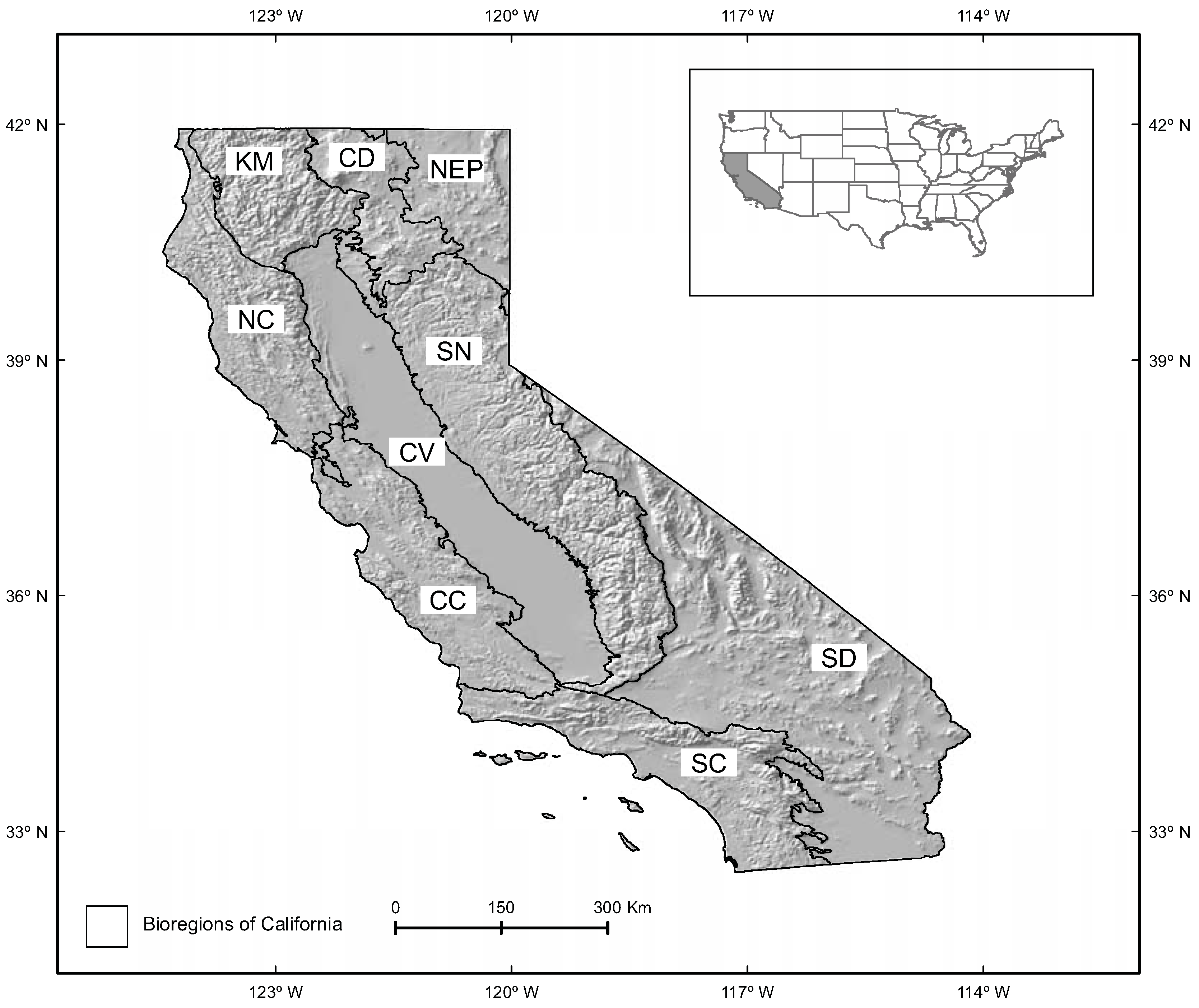
2.1. Study Area
2.2. Fire and Watershed Data
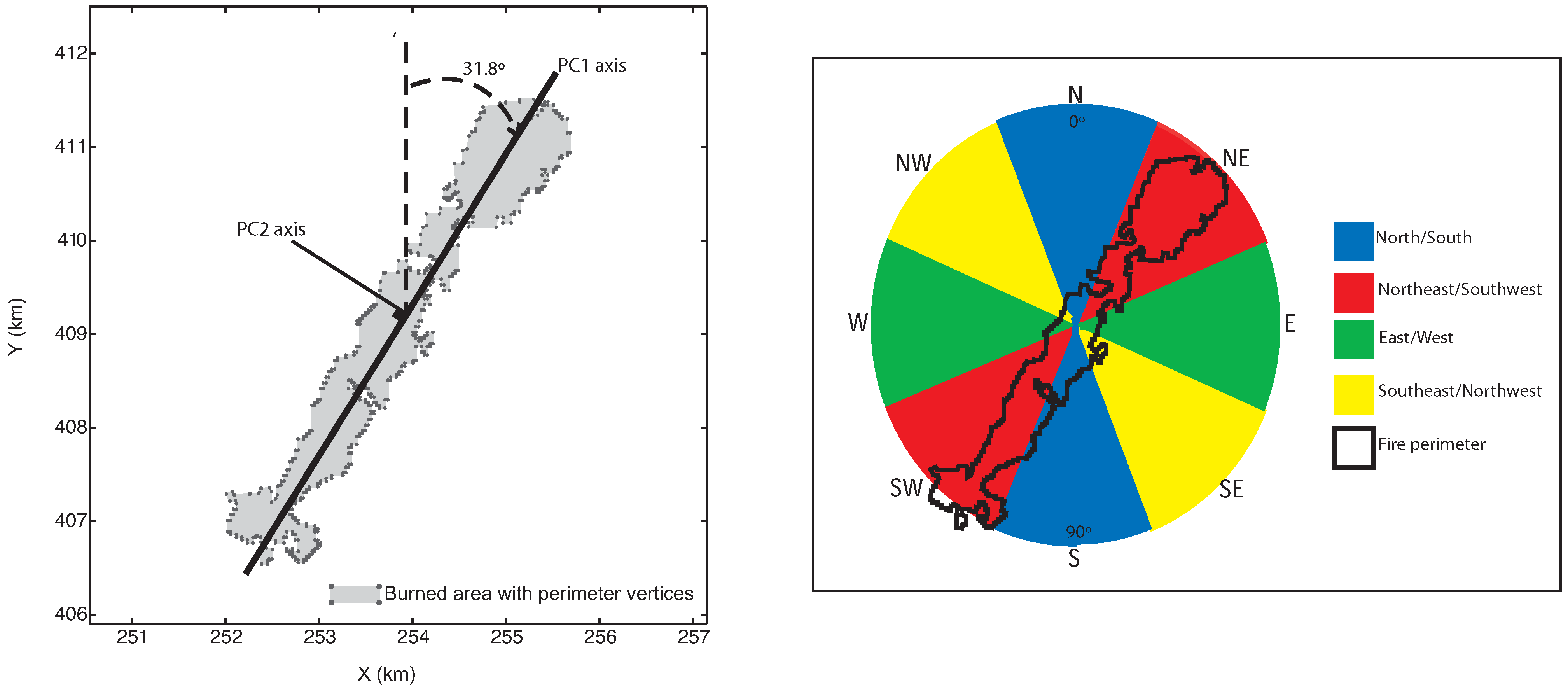
2.3. Circular Statistics Analysis


| Test | Hypothesis | Circular distributions |
|---|---|---|
| Kuiper | H0 | Uniform |
| H1 | Not uniform | |
| Watson | H0 | von Mises |
| H1 | Not von Mises | |
| Rayleigh | H0 | Uniform |
| H1 | Unimodal |
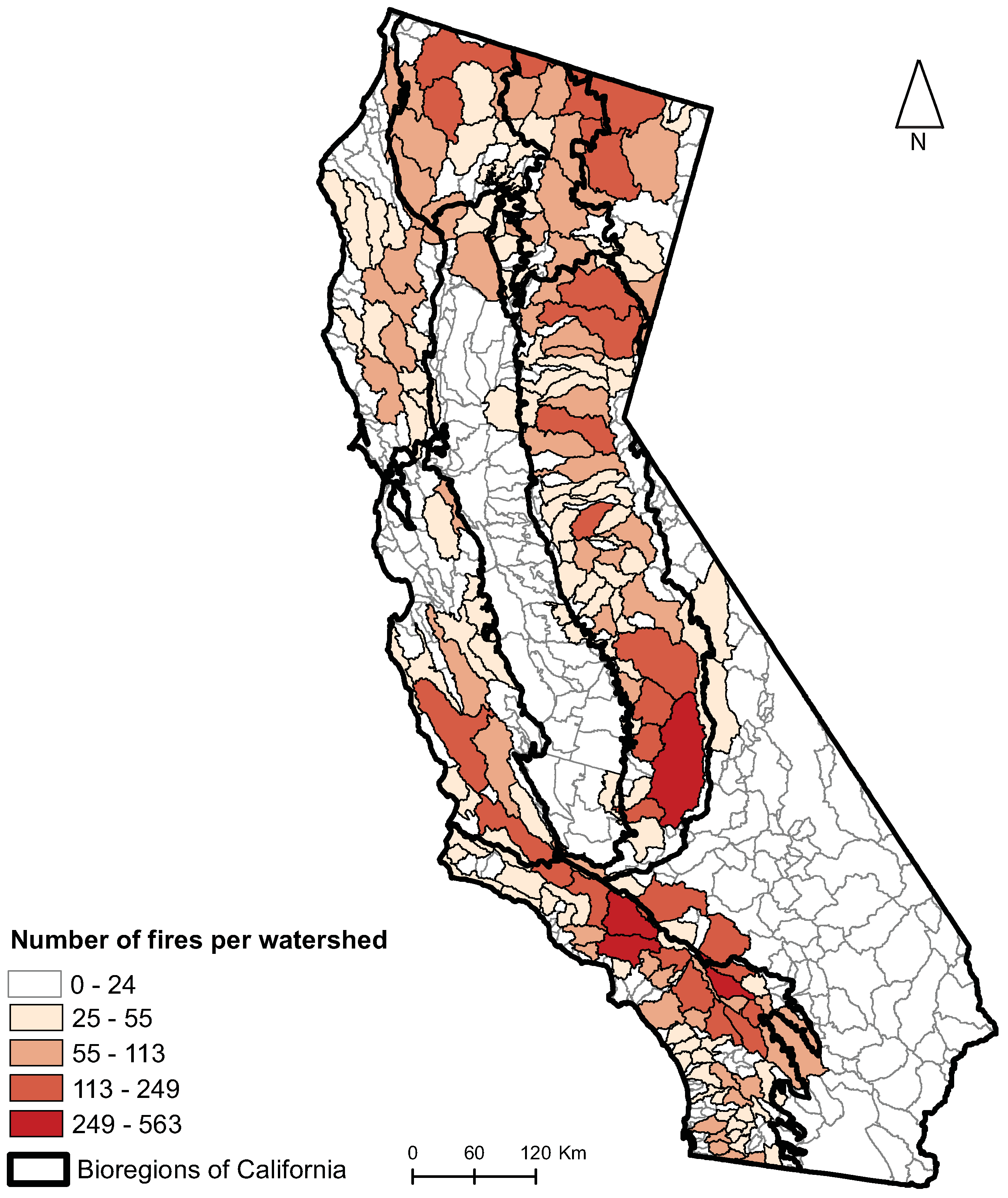
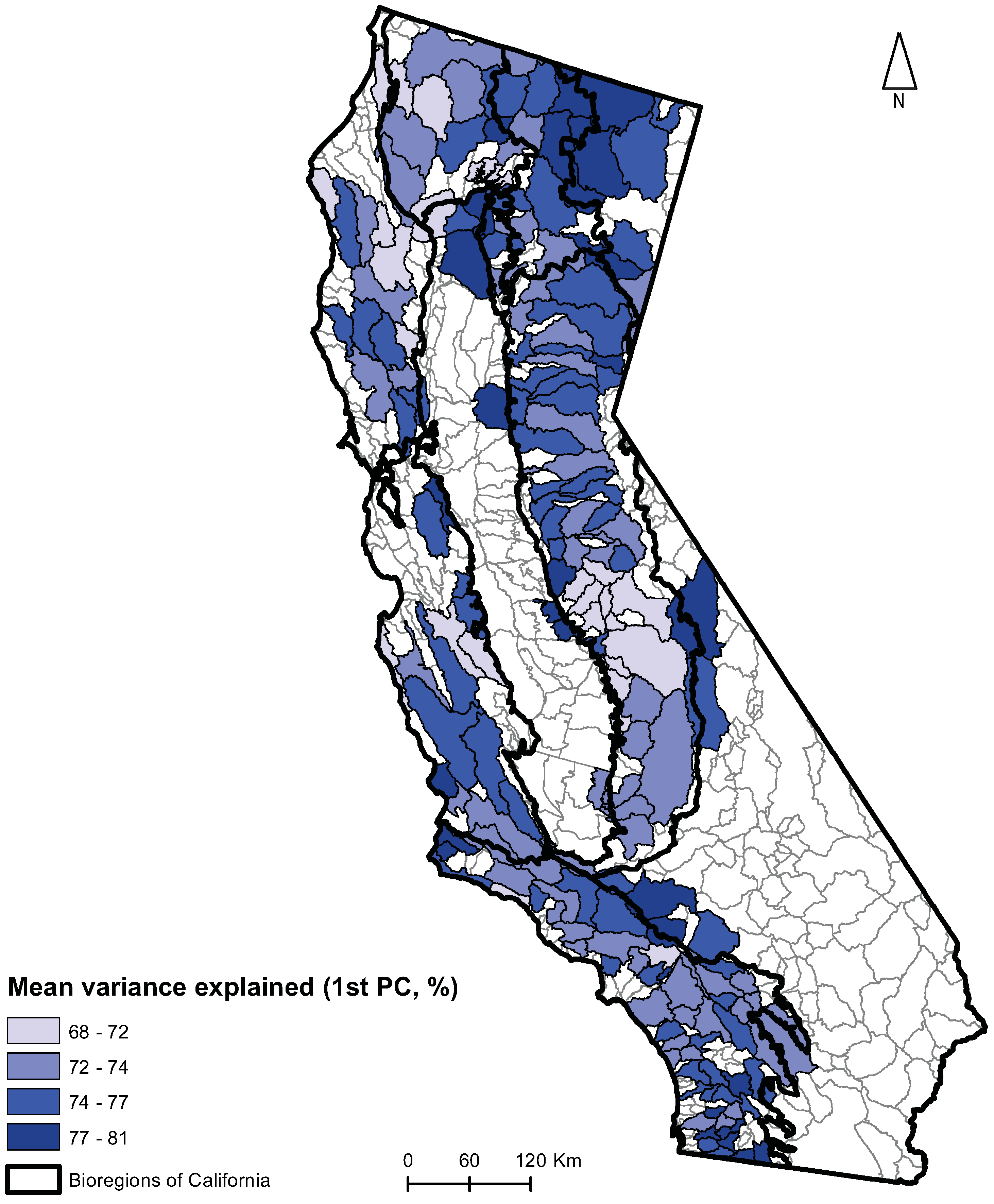
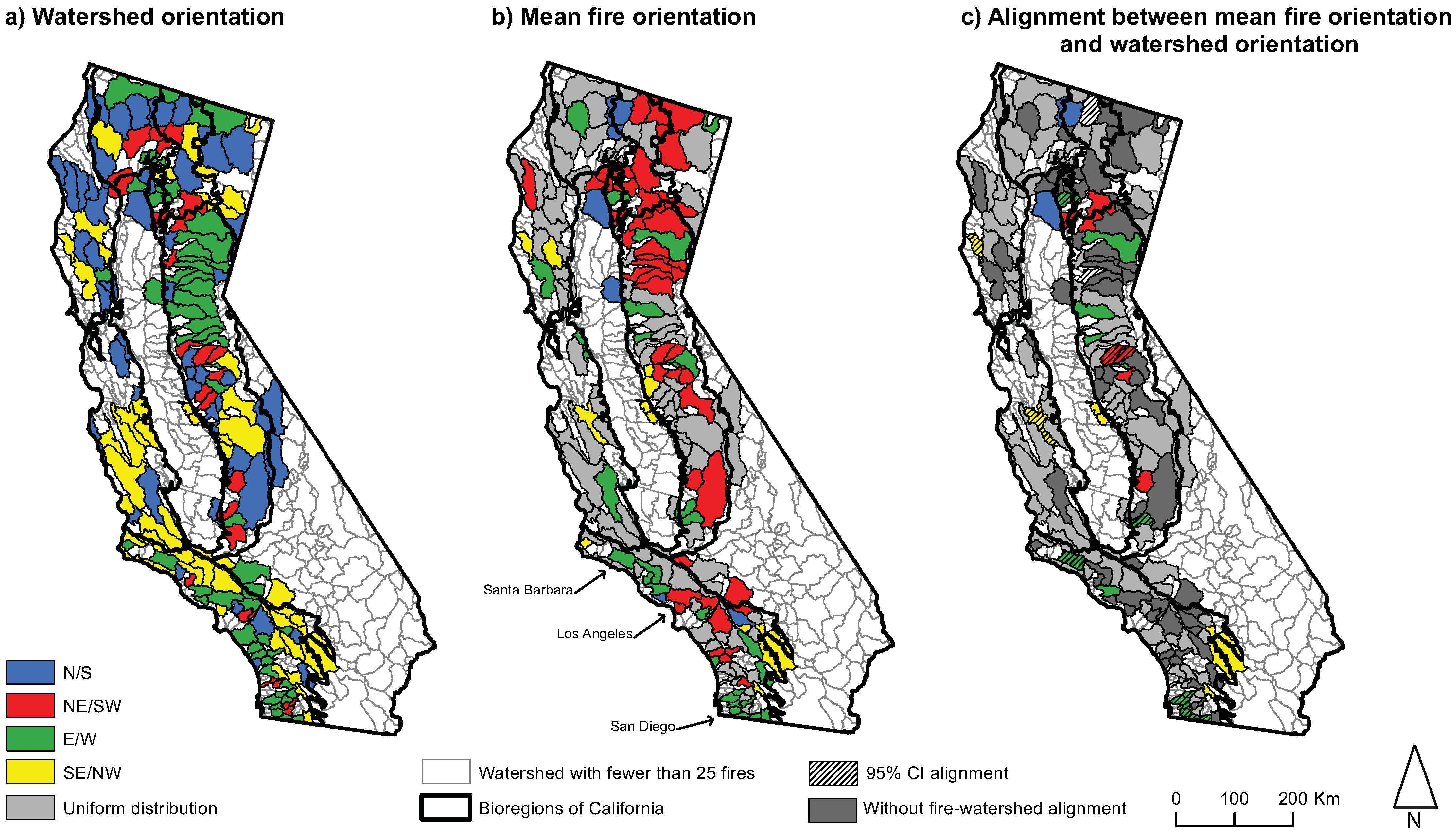
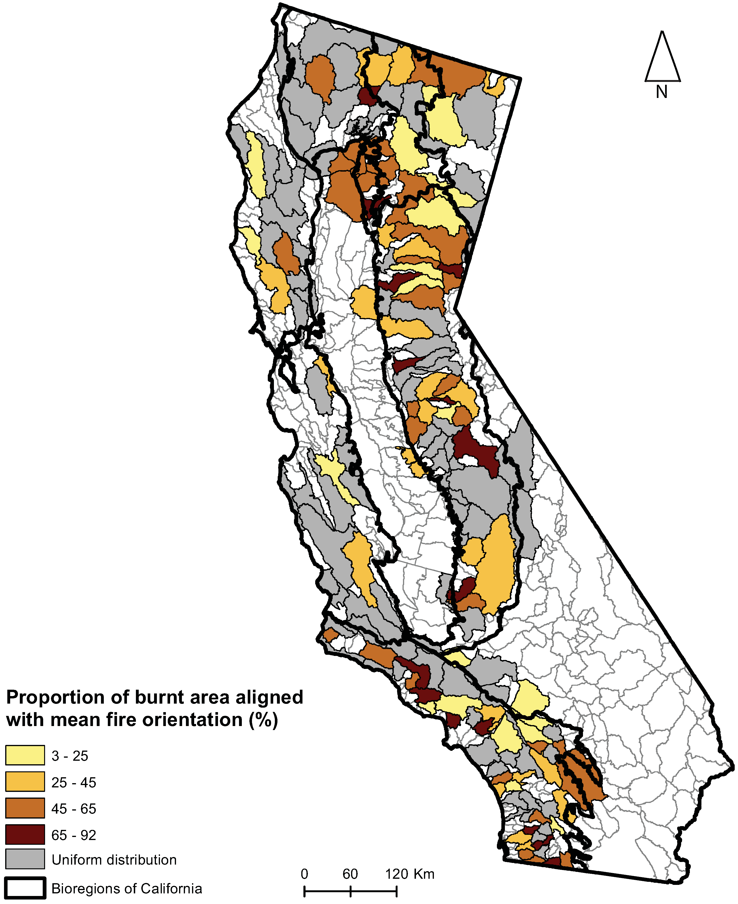
3. Results


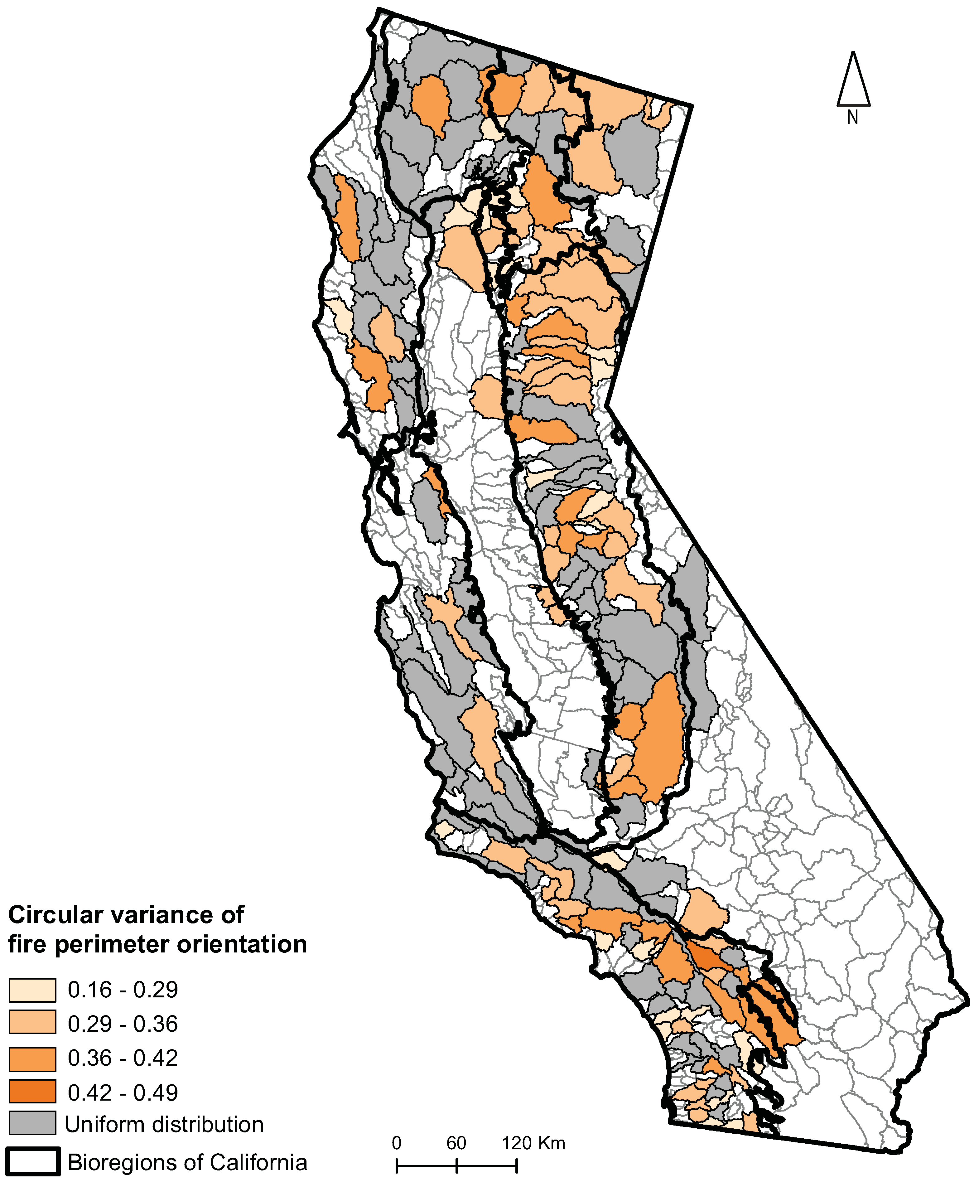

4. Discussion
Acknowledgments
References
- Stocks, B.; Mason, J.; Todd, J.; Bosch, E.; Wotton, B.; Amiro, B.; Flannigan, M.; Hirsch, K.; Logan, K.; Martell, D.; Skinner, W. Large forest fires in Canada, 1959–1997. J. Geophys. Res. 2002, 108, 1–12. [Google Scholar] [CrossRef]
- Sugihara, N.; van Wagdentonk, J.; Shaffer, K.; Fites-Kaufman, J.; Thode, A. Fire in California’s Ecosystem; University of California Press: Berkeley, CA, USA, 2006; p. 583. [Google Scholar]
- Tedim, F.; Remelgado, R.; Borges, C.; Carvalho, S.; Martins, J. Exploring the occurrence of mega-fires in Portugal. For. Ecol. Manag. 2012, 294, 86–96. [Google Scholar] [CrossRef]
- Ganteaume, A.; Jappiot, M. What causes large fires in Southern France? For. Ecol. Manag. 2012, 294, 76–85. [Google Scholar] [CrossRef]
- Bradstock, R. Effects of large fires on biodiversity in southern-eastern Australia: Disaster or template for diversity? Int. J. Wildland Fire 2008, 17, 809–822. [Google Scholar] [CrossRef]
- Gill, A.; Stephens, S. Scientific and social challenges for the management of fire-prone wildland-urban interfaces. Environ. Res. Lett. 2004, 3, 1–10. [Google Scholar] [CrossRef]
- Stephens, S.; Adams, M.; Handmer, J.; Kearns, F.; Leicester, B.; Leonard, J.; Moritz, M. Urban-wildland fires: How California and other regions of the US can learn from Australia. Environ. Res. Lett. 2009, 4, 1–5. [Google Scholar] [CrossRef]
- Penman, T.; Christie, F.; Andersen, A.; Bradstock, R.; Cary, G.; Henderson, M.; Price, O.; Tran, C.; Wardle, G.; Williams, R.; Tork, A. Prescribed burning: How can it work to conserve the things we value? Int. J. Wildland Fire 2011, 20, 721–733. [Google Scholar] [CrossRef]
- Spies, T.; Lindenmayer, D.; Gill, A.; Stephens, S.; Agee, J. Challenges and a checklist for biodiversity conservation in fire-prone forests: Perspectives from the Pacific Northwest of USA and Southeastern Australia. Biol. Conserv. 2012, 145, 5–14. [Google Scholar] [CrossRef]
- Hardy, C. Wildland fire hazard and risk: Problems, definitions, and context. For. Ecol. Manag. 2005, 211, 73–82. [Google Scholar] [CrossRef]
- Keely, J.; Bond, W.; Bradstock, R.; Pausas, J.; Rundel, P. Fire in California. In Fire in Mediterranean Ecosystems. Ecology, Evolution and Management; Cambridge University Press: New York, NY, USA, 2012; pp. 113–149. [Google Scholar]
- Sugihara, N.; Barbour, M. Fire and California Vegetation. In Fire in California’s Ecosystem; Sugihara, N., van Wagdentonk, J., Shaffer, K., Fites-Kaufman, J., Thode, A., Eds.; University of California Press: Berkeley, CA, USA, 2006; pp. 391–414. [Google Scholar]
- Radeloff, V.; Hammer, R.; Stewart, S.; Fried, J.; Holcomb, S.; McKeefry, J. The wildland urban interface in the United States. Ecol. Appl. 2005, 15, 799–805. [Google Scholar] [CrossRef]
- Syphard, A.; Radeloff, V.; Keeley, J.; Hawbaker, T.; Clayton, M.; Stewart, S.; Hammer, R. Human influence on California fire regimes. Ecol. Appl. 2007, 17, 1388–1402. [Google Scholar] [CrossRef] [PubMed]
- Syphard, A.; Radeloff, V.; Hawbaker, T.; Stewart, S. Conservation threats due to human-caused increases in fire frequency in mediterranean-climate ecosystems. Conserv. Biol. 2009, 23, 758–769. [Google Scholar] [CrossRef] [PubMed]
- Stephens, S.; Moghaddas, J.; Edminster, C.; Fiedler, C.; Haase, S.; Harrington, M.; Keeley, J.; Knapp, E.; McIver, J.; Metlen, K.; et al. Fire treatment effects on vegetation structure, fuels, and potential fire severity in western U.S. forests. Ecol. Appl. 2009, 19, 305–320. [Google Scholar] [CrossRef] [PubMed]
- Minnich, R. California Climate and Fire Weather. In Fire in California’s Ecosystem; Sugihara, N., van Wagdentonk, J., Shaffer, K., Fites-Kaufman, J., Thode, A., Eds.; University of California Press: Berkeley, CA, USA, 2006; pp. 13–28. [Google Scholar]
- Albini, F.; Brown, J.; Reinhardt, E.; Ottmar, R. Calibration of a large burnout model. Int. J. Wildland Fire 1995, 5, 173–192. [Google Scholar] [CrossRef]
- van Wagtendonk, J. Fire and a Physical Process. In Fire in California’s Ecosystem; Sugihara, N., van Wagdentonk, J., Shaffer, K., Fites-Kaufman, J., Thode, A., Eds.; University of California Press: Berkeley, CA, USA, 2006; pp. 38–57. [Google Scholar]
- Werth, P. Critical Fire Weather Patterns. In Synthesis of Knowledge of Extreme Fire Behavior: Volume I for Fire Managers; USDA Forest Service: Portland, OR, USA, 2011; pp. 147–169. [Google Scholar]
- Green, L. Fuelbreaks and Other Fuel Modification for Wildland Fire Control. In US Department of Agriculture and Forest, Forest Service Agricultural Handbook; US Forest Service: Washington, DC, USA, 1977; Volume 499, pp. 1–85. [Google Scholar]
- Agee, J.; Bahro, B.; Finney, M.; Omi, P.; Sapsis, D.; Skinner, C.; van Wagtendonk, J.; Weatherspoon, C.P. The use of shaded fuelbreaks in landscape fire management. For. Ecol. Manag. 2000, 127, 55–66. [Google Scholar] [CrossRef]
- Agee, J.; Skinner, C. Basic principles of forest fuel reduction treatments. For. Ecol. Manag. 2005, 211, 83–96. [Google Scholar] [CrossRef]
- Moghaddas, J.; Collins, B.; Menning, K.; Moghaddas, E.; Stephens, S. Fuel treatment effects on modeled landscape-level fire behavior in the northern Sierra Nevada. Can. J. For. Res. 2010, 40, 1751–1765. [Google Scholar] [CrossRef]
- Ager, A.; Vaillant, N.; Finney, M. A comparison of landscape fuel treatment strategies to mitigate wildland fire risk in the urban interface and preserve old forest structure. For. Ecol. Manag. 2010, 259, 1556–1570. [Google Scholar] [CrossRef]
- Price, O.; Bradstock, R. The efficacy of fuel treatment in mitigating property loss during wildfires: Insights from analysis of the severity of the catastrophic fires in 2009 in Victoria, Australia. J. Environ. Manag. 2012, 113, 146–157. [Google Scholar] [CrossRef] [PubMed]
- Bradstock, R.; Cary, G.; Davies, I.; Lindenmayer, D.; Price, O.; Williams, R. Wildfires, fuel treatment and risk mitigation in Australian eucalypt forests: Insights from landscape-scale simulation. J. Environ. Manag. 2012, 105, 66–75. [Google Scholar] [CrossRef] [PubMed]
- Weatherspoon, C.; Skinner, C. Landscape-Level Strategies for Forest Fuel Management. In Sierra Nevada Ecosystem Project: Final Report to Congress; University of California, Davis, Centers for Water and Wildland resources: Davis, CA, USA, 1996; Volume 2, pp. 1471–1492. [Google Scholar]
- Duguy, B.; Alloza, J.; Roder, A.; Vallejo, R.; Pastor, F. Modelling the effects of landscape fuel treatments on fire growth and behaviour in a Mediterranean landscape (eastern Spain). Int. J. Wildland Fire 2007, 16, 619–632. [Google Scholar] [CrossRef]
- Finney, M. Design of regular landscape fuel treatment patterns for modifying fire growth and behavior. For. Sci. 2001, 47, 219–228. [Google Scholar]
- Loehle, C. Applying landscape principles to fire hazard reduction. For. Ecol. Manag. 2004, 198, 261–267. [Google Scholar] [CrossRef]
- Finney, M.; Seli, R.; McHugh, C.; Ager, A.; Bahro, B.; Agee, J. Simulation of long-term landscape-level fuel treatment effects on large wildfires. Int. J. Wildland Fire 2007, 16, 712–727. [Google Scholar] [CrossRef]
- Schmidt, D.; Taylor, A.; Skinner, C. The influence of fuels treatment and landscape arrangement on simulated fire behavior, Southern Cascade range, California. For. Ecol. Manag. 2008, 255, 3170–3184. [Google Scholar] [CrossRef]
- Barros, A.; Pereira, J.; Lund, U. Identifying geographical patterns of wildfire orientation: A watershed-based analysis. For. Ecol. Manag. 2012, 264, 98–107. [Google Scholar] [CrossRef]
- Haydon, D.; Friar, J.; Pianka, E. Fire-driven dynamic mosaics in the Great Victoria Desert, Australia-Fire geometry. Landsc. Ecol. 2000, 15, 373–381. [Google Scholar] [CrossRef]
- Bergeron, Y.; Gauthier, S.; Flannigan, M.; Kafka, V. Fire regimes at the transition between mixedwood and coniferous boreal forest in Northwestern Quebec. Ecology 2004, 85, 1976–1932. [Google Scholar] [CrossRef]
- Parisien, M.; Peters, V.; Wang, Y.; Little, J.; Bosch, E.; Stocks, B. Spatial patterns of forest fires in Canada, 1980–1999. Int. J. Wildland Fire 2006, 15, 361–374. [Google Scholar] [CrossRef]
- Viegas, D. Parametric study of an eruptive fire behaviour model. Int. J. Wildlandf Fire 2006, 15, 169–177. [Google Scholar] [CrossRef]
- Bailey, R. Ecosystem Geography: From Ecoregions to Sites; Springer: New York, NY, USA, 1996; p. 243. [Google Scholar]
- Miles, S.; Goudey, C. Ecological Subregions of California: Section and Subsection Descriptions; USDA Forest Service: San Francisco, CA, USA, 1997.
- Stuart, J.; Stephens, S. North Coast Bioregion. In Fire in California’s Ecosystem; Sugihara, N., van Wagdentonk, J., Shaffer, K., Fites-Kaufman, J., Thode, A., Eds.; University of California Press: Berkeley, CA, USA, 2006; pp. 147–169. [Google Scholar]
- Keely, J. South Coast Bioregion. In Fire in California’s Ecosystem; Sugihara, N., van Wagdentonk, J., Shaffer, K., Fites-Kaufman, J., Thode, A., Eds.; University of California Press: Berkeley, CA, USA, 2006; pp. 350–390. [Google Scholar]
- Skinner, C.; Agee, J. Klamath Mountains Bioregion. In Fire in California’s Ecosystem; Sugihara, N., van Wagdentonk, J., Shaffer, K., Fites-Kaufman, J., Thode, A., Eds.; University of California Press: Berkeley, CA, USA, 2006; pp. 170–194. [Google Scholar]
- Skinner, C.; Taylor, A. Southern Cascades Bioregion. In Fire in California’s Ecosystem; Sugihara, N., van Wagdentonk, J., Shaffer, K., Fites-Kaufman, J., Thode, A., Eds.; University of California Press: Berkeley, CA, USA, 2006; pp. 195–224. [Google Scholar]
- Riegel, G.; Miller, R.; Skinner, C.; Smith, S. Northeastern Plateau Bioregion. In Fire in California’s Ecosystem; Sugihara, N., van Wagdentonk, J., Shaffer, K., Fites-Kaufman, J., Thode, A., Eds.; University of California Press: Berkeley, CA, USA, 2006; pp. 225–263. [Google Scholar]
- Wills, R. Central Valley Bioregion. In Fire in California’s Ecosystem; Sugihara, N., van Wagdentonk, J., Shaffer, K., Fites-Kaufman, J., Thode, A., Eds.; University of California Press: Berkeley, CA, USA, 2006; pp. 295–320. [Google Scholar]
- Brooks, M.; Minnich, R. Southeastern Deserts Bioregion. In Fire in California’s Ecosystem; Sugihara, N., van Wagdentonk, J., Shaffer, K., Fites-Kaufman, J., Thode, A., Eds.; University of California Press: Berkeley, CA, USA, 2006; pp. 391–414. [Google Scholar]
- Pyne, S.; Andrews, P.; Laven, R. Introduction to Wildland Fire; John Wiley and Sons: New York, NY, USA, 1996; p. 808. [Google Scholar]
- FRAP. Fire Perimeters, Version 10.1 ed; California Department of Forestry and Fire Protection: Sacramento, CA, USA, 2011. [Google Scholar]
- FRAP. California Interagency Watershed Map of 1999 CalWater, Version 2.2.1 ed; California Department of Forestry and Fire Protection: Sacramento, CA, USA, 2004. [Google Scholar]
- Fisher, N. Statistical Analysis of Circular Data; Cambridge University Press: Cambridge, England, UK, 1995; p. 296. [Google Scholar]
- Luo, D. Pattern Recognition and Image Processing; Horwood Publishing: Chichester, England, UK, 1998; p. 245. [Google Scholar]
- Mardia, K.; Jupp, P. Directional Statistics; John Wiley and Sons: Chichester, England, UK, 2000; p. 415. [Google Scholar]
- Kovach, W. Oriana. In Circular Statistics for Windows, Version 2 ed; Kovach Computing Services: Pentraeth, Wales, UK, 2003. [Google Scholar]
- Strauss, D.; Bednar, L.; Mees, R. Do one percent of forest fires cause ninety-nine percent of the damage? For. Sci. 1989, 35, 319–328. [Google Scholar]
- Openshaw, S. The modifiable areal unit problem. Concepts Tech. Mod. Geogr. 1984, 38, 173–192. [Google Scholar]
- Marceau, D. The scale issue in social and natural sciences. Can. J. Remote Sens. 1999, 25, 347–356. [Google Scholar] [CrossRef]
- Hull, M.; O’Dell, C.; Schroeder, M. Critical Fire Weather Patterns-Their Frequency and Levels of Fire Danger; US Department of Agriculture, Forest Service, Pacific Southwest Forest and Range Experiment Station: Berkeley, CA, USA, 1966.
- Clements, C. Mountain and valley winds of Lee Vining Canyon, Sierra Nevada, California, USA. Artic Antartic Alpine Res. 1999, 31, 293–302. [Google Scholar] [CrossRef]
- Clements, C. Effects of Complex Terrain on Extreme Fire Behavior. In Synthesis of Knowledge of Extreme Fire Behavior: Volume I for Fire Managers; USDA Forest Service: Portland, OR, USA, 2011; pp. 147–169. [Google Scholar]
- Whiteman, C. Mountain Meteorology: Fundamentals and Applications; Oxford University Press: New York, NY, USA, 2000; p. 358. [Google Scholar]
- Minnich, R. An integrated model of two fire regimes. Conserv. Biol. 2001, 15, 1549–1553. [Google Scholar] [CrossRef]
- Keely, J.; Fotheringham, C. Historic fire regime in Southern California Shrublands. Conserv. Biol. 2001, 15, 1536–1548. [Google Scholar] [CrossRef]
- Moritz, M.; Moody, T.; Krawchuk, M.; Hughes, M.; Hall, A. Spatial variation in extreme winds predicts large wildfire locations in chaparral ecosystems. Geophys. Res. Lett. 2010, 37, 1–5. [Google Scholar] [CrossRef]
- Xu, H.; Nichols, K.; Schoenberg, F. Kernel regression of directional data with application to wind and wildfire data in Los Angeles county, California. For. Sci. 2011, 7, 343–352. [Google Scholar]
- Raphael, M. The Santa Ana winds of California. Earth Interact. 2003, 7, 1–8. [Google Scholar] [CrossRef]
- Westerling, A.; Cayan, D.; Brown, T.; Hall, B.; Riddle, L. Climate, Santa Ana winds and autumn wildfires in Southern California. Eos 2004, 85, 1–4. [Google Scholar] [CrossRef]
- Hughes, M.; Hall, A. Local and synoptic mechanisms causing Southern California’s Santa Ana winds. Clim. Dyn. 2010, 34, 847–857. [Google Scholar] [CrossRef]
- Campbell, A. Sonora storms and Sonora clouds of California. Mon. Weather Rev. 1906, 34, 464–465. [Google Scholar] [CrossRef]
- Sommers, W. LFM forecast variables related to santa ana wind occurrences. Mon. Weather Rev. 1978, 106, 1307–1316. [Google Scholar] [CrossRef]
- Ryan, G. Sundowner Winds; Weather Service Office: Santa Maria, CA, USA, 1991; p. 18. [Google Scholar]
- Keeley, J.; Fotheringham, C.; Moritz, M. Lessons from the October 2003. Wildfires in Southern California. J. For. 2004, 102, 26–31. [Google Scholar]
- Keely, J.; Safford, H.; Fotheringham, C.; Franklin, J.; Moritz, M. The 2007 Southern California Wildfires: Lessons in complexity. J. For. 2009, September, 287–296. [Google Scholar]
- Collins, B.; Stephens, S.; Moghaddas, J.; Battles, J. Challenges and approaches in planning fuel treatments across fire-excluded forested landscapes. J. For. 2010, January/February, 24–31. [Google Scholar]
© 2013 by the authors; licensee MDPI, Basel, Switzerland. This article is an open access article distributed under the terms and conditions of the Creative Commons Attribution license (http://creativecommons.org/licenses/by/3.0/).
Share and Cite
Barros, A.M.G.; Pereira, J.M.C.; Moritz, M.A.; Stephens, S.L. Spatial Characterization of Wildfire Orientation Patterns in California. Forests 2013, 4, 197-217. https://doi.org/10.3390/f4010197
Barros AMG, Pereira JMC, Moritz MA, Stephens SL. Spatial Characterization of Wildfire Orientation Patterns in California. Forests. 2013; 4(1):197-217. https://doi.org/10.3390/f4010197
Chicago/Turabian StyleBarros, Ana M.G., José M.C. Pereira, Max A. Moritz, and Scott L. Stephens. 2013. "Spatial Characterization of Wildfire Orientation Patterns in California" Forests 4, no. 1: 197-217. https://doi.org/10.3390/f4010197
APA StyleBarros, A. M. G., Pereira, J. M. C., Moritz, M. A., & Stephens, S. L. (2013). Spatial Characterization of Wildfire Orientation Patterns in California. Forests, 4(1), 197-217. https://doi.org/10.3390/f4010197