Abstract
Skidding is one of the most important methods for wood extraction globally, necessitating updated models to assess its performance based on the technical characteristics of the fleet in use. Based on a nation-wide, all-season dataset, this paper aimed to develop time and fuel consumption models for currently used cable skidders and farm tractors fitted for skidding in Romania. Although some statistical assumptions were not met, our models characterized the performance well in terms of time and fuel consumption, allowing for a differentiation in performance between skidders and farm tractors. For skidders, cycle time was explained to a degree of 58% (R2 = 0.58) by payload volume, number of pieces, and extraction distance, highlighting the importance of these variables when assessing cycle time performance of machines equipped with a double-drum winch. In contrast, for farm tractors, cycle time was explained solely by extraction distance (R2 = 0.87), which indicates a lower variability induced by payload size and number of pieces for machines equipped with a single-drum winch. Similar models were developed for fuel consumption, showing the significance of payload volume and extraction distance for skidders (R2 = 0.54) and extraction distance alone (R2 = 0.75) for farm tractors. Beyond an extraction distance of 50 m, the productivity of farm tractors decreased sharply, reaching half of that of skidders at an extraction distance of 1500 m, indicating a better time and fuel consumption performance of skidders, particularly in the case of excessively long extraction distances. Further studies should focus on finding effective methods and developing automated systems able to track the performance of operations and keep the pace with improvements in machine performance.
Keywords:
time-and-motion; work elements; skidders; farm tractors; models; prediction; performance; fuel use; nation-wide 1. Introduction
Ground-based timber harvesting encompasses a wide range of operational systems, ranging from manual to fully mechanized methods. Skidding using specialized machines and farm tractors constitutes a significant share of practices at both the global [1] and European levels [2]. Cable skidders are machines equipped with a winch, typically used to pull the wood from the stand to a trail by cables, where the payload is then secured for extraction to the forest road; farm tractors equipped with a winch for forest operations are similar to cable skidders in terms of operational function but differ in their capacity and construction design [3,4,5].
Understanding the performance of skidding operations is important for several levels of decision-making. At the strategic and tactical levels, efficiency, productivity, and fuel use are factors that inform decisions about the most suitable machines for a given area [6]. Additionally, assessment on fuel consumption is critical in forest operations [7] because it may impact policies and decision-making related to climate change and the carbon neutrality of human-made systems [8], which may involve decisions regarding the types of machines and processes to be employed. Accordingly, it has received considerable attention in forest engineering, by studies based on census data, e.g., [9,10], or direct measurement, e.g., [11,12].
Furthermore, forestry encompasses many processes and levels of decision-making, where the performance of some may affect the decisions regarding others. For instance, planning and developing the forest road network typically requires information about the systems used or forecasted in timber harvesting and their performance [13,14], which is generally expressed in the form of models developed by time and motion studies [15]. In other cases, the developed productivity models are useful to understand the technical limitations of machines in relation to their operational environment [16]. For a forest company, performance models are important for its business design and practice; at the operational level, they are useful for operational planning, understanding cost trends [17] and setting up fair compensation systems [3,6].
Modeling of skidding performance has received considerable attention in the dedicated literature, by developing time and fuel consumption models for cable skidders and farm tractors equipped for cable skidding. For instance, studies of [18,19,20,21,22,23,24,25] focused mainly on providing statistics and models of time consumption and productivity, whereas the studies of [26,27,28] included fuel use assessments at various scales to model and characterize fuel consumption, energy efficiency, and emissions. Such models, however, have limitations, and their validity is constrained by the range of data used to develop them, local practices, and the type of forest management. These factors prevent their generalizability to other areas of the world [29]. In addition, many of these models were developed considering a single work team and harvesting site, which means they incorporate limited variability in terms of operator experience, as well as stand and terrain factors. Other important factors that relate to a limited generalizability of the developed models include the size of the samples used, the accuracy of estimates regarding time consumption, production, fuel use, and the range of operational factors such as extraction distance. Additionally, collecting long-term data and using it to develop models may help mitigate bias induced by the season in which data is collected. For instance, the condition of the trails used for skidding, which in turn influences machine performance, as well as performance during pre-skidding with a winch, may be affected by the season, weather, and ground state.
In Romania, cable skidders and farm tractors equipped for skidding dominate the practice of timber harvesting, e.g., [2,3,30]. This situation is related to factors such as the availability of local machine manufacturers that release machines on the market at competitive prices, the tradition of cable skidding, and compatibility with motor-manual tree felling and processing procedures, which are commonly used. Additionally, cable skidding requires a lower level of operational skills compared to cable yarding. However, in many cases, it requires a well-developed network of skid roads and trails [3,21]. Local manufacturers have released new models of skidders, whereas the old Romanian-made farm tractors used in forest operations have been gradually replaced with affordable, mostly foreign models. As of now, there are at least three newer domestic cable skidder models operating in the Romanian forests, along with several imported farm tractors. However, the available performance models have not kept pace with technological development, making the decision-making process difficult. For instance, the new machines are equipped with improved engines that deliver increased power while consuming less fuel, whereas the latest aggregated productivity rates in timber harvesting date back to the 1990s [31].
This study aimed to develop time and fuel consumption models for the commonly used cable skidders and farm tractors equipped for skidding in Romania, as a prerequisite for modeling their efficiency, productivity, and unit fuel use based on a comprehensive dataset that is representative at the national level. The main goal was to develop a set of models able to characterize the operational performance at the national level. The objectives of the study were to: (i) model the skidding cycle time as a function of relevant factors such as extraction distance, payload volume, and the number of skidded wood pieces; (ii) model fuel consumption as a function of relevant factors such as extraction distance, payload volume, and the number of skidded wood pieces; and (iii) estimate and model the efficiency, productivity and unit fuel consumption of skidding based on the developed time and fuel consumption models.
2. Materials and Methods
2.1. Study Locations and Machine Types
A comprehensive data set was collected for cable skidders and farm tractors at the national level (Figure 1). This data set consists of detailed time consumption and location information, documented using state-of-the-art video cameras (GoPro HERO series, GoPro Inc., San Mateo, CA, USA) mounted on the rear of the machines, as well as handheld GNSS receivers (Garmin GPSMAP series, Garmin International Inc., Olathe, KS, USA) placed on the machine cabs. The initial dataset included 304 work cycles for cable skidders collected over a 71 day period and 117 work cycles for farm tractors equipped for skidding, collected over a 16 day period (Table 1).
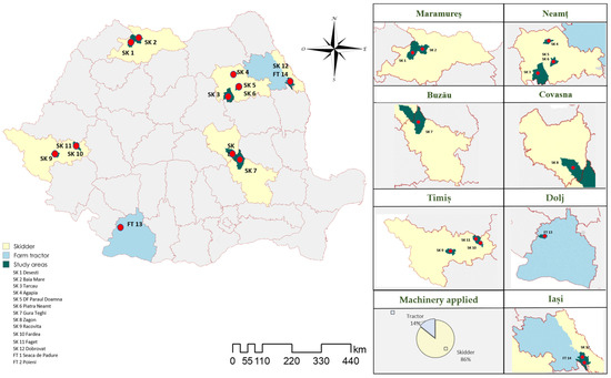
Figure 1.
Map of Romania showing the locations of the data collection counties and local study areas. Note: SK—study location for cable skidders, FT—study location for farm tractors. Note: the names of the counties and study areas are reported in Romanian.

Table 1.
Description of the initial dataset.
Both machine types (Table 1) were classified in the same power-rating category according to [32], specifically up to 80 kW. The skidder category included, with one exception (an older Romanian model TAF 657, 48 kW), the Romanian-made TAF 690 OP (70 kW). In contrast, the farm tractor category included machines within the same power-rating class—Zetor Proxima (series CL 59–74 kW). With respect to trail condition, moist trails characterized all observations where the ground exhibited moisture, such as muddy terrain or ground covered with melted snow. In contrast, dry trails included all observations where the ground was in a dried state (Figure A1). The forest type category encompassed beech forests, as well as forests featuring various broadleaved species (Broadleaved), mixed forests containing different proportions of coniferous and broadleaved trees (Mixed), and Norway spruce forests (Coniferous). It is important to note that data regarding species share, tree size, and terrain slope was not specifically collected for this study.
The data was collected from 14 sites distributed throughout Romania, encompassing a variety of conditions related to forest type, age, tree size, ground conditions, and work season. Skidders were observed in 12 study areas, primarily in steep, hilly, and mountainous terrain—cases in which the work teams were dominantly composed of 3 workers. Farm tractors were observed at 2 sites characterized by moderate to low slopes in the hilly and plain regions of the country; in these cases, the work teams were composed mostly of 2 workers. The dominant harvesting method for cable skidders was tree length, while both tree-length and cut-to-length methods were utilized with farm tractors.
2.2. Data Collection
The video cameras were strategically placed at the back of the machines to provide a panoramic view of the operations, allowing for a comprehensive recording of all tasks carried out during the process. They were set to continuously collect high-resolution video data in files approximately 20 min in length. To extend battery life, the cameras were connected to portable power banks. For accurate measurement of distances traveled and precise location tracking, the receivers were configured to record geospatial information at a rate of one second. By adjusting the devices’ parameters, it was verified that they were in continuous tracking mode, enabling data collection throughout the sampling period.
For each piece within a work cycle-based payload, diameter sampling was conducted at intervals of 0.5 m using a caliper and measuring tape. This data was recorded on paper sheets and subsequently used to compute the volume of each piece and the entire payload during the office phase of the study. The data was collected at the landing once the payload was detached from the machine after each observed work cycle.
The evaluation of fuel consumption was conducted at the end of each work cycle using a graded and calibrated plastic container (shaped like a jar for ease of use) to ensure accurate measurements. At the beginning of each work cycle, the machine’s fuel tank was filled to capacity, which allowed for the recording of the amount of fuel consumed during that cycle once the tank was refilled. Fuel consumption measurement tasks were carried out in the same location on the site, specifically on a leveled portion of the landing, to ensure accurate readings.
2.3. Data Processing
Data processing consisted of several steps. All data were classified by day, creating folders that contained recorded videos, GNSS data, fuel consumption figures, and diameter measurements. The data were organized in Microsoft Excel to create a spreadsheet for each study site. Each sheet contained specific data for the days on which information was collected in that area. During the review of video files, relevant data were extracted, including the day, video code, log number, start time, end time, effective time, task code (Table 2), and any comments regarding unusual observations. This activity primarily focused on extracting the time in seconds dedicated to each task during the work cycle, as well as refining the data to remove those work cycles that were not fully documented by video and GNSS data. After these steps, 182 work cycles for skidders and 45 work cycles for farm tractors were preserved for further processing and included in dedicated spreadsheets.
Table 2.
Description of the time consumption categories observed in the datasets.
With the help of the Garmin BaseCamp software (v. 4.7.4), the distances traveled cycle-wise by the observed machines were determined using the methodology proposed by [28], which included a detailed and synchronized analysis of GNSS tracks in Garmin Base Camp software (v. 4.7.4) coupled with data documentation based on video files for each single data registry collected by GNSS devices. Accordingly, GNSS tracks were examined on a daily and work cycle basis to determine the distances travelled from the landing area to the pre-skidding site and back, as well as the extraction distance.
The final database included cycle-wise elemental time consumption for the elements described in Table 2, driving distances, including the average extraction distance (AED, m), number of pieces per turn, payload volume (PV, m3), and cycle-wise fuel consumption estimates (FC, L).
2.4. Statistical Analysis
Statistical analysis was conducted on the refined dataset, which included 182 work cycles for skidders and 45 work cycles for farm tractors. For both datasets, the following sequence of statistical analysis steps was implemented, taking as a reference the work of [33,34]:
- The variables of elemental time consumption (tDET, tMAN, tPOC, tAPL, tPIP, tDPC, tAPE, tDFR, tDPR, tMBR, tDS, tDP, tDM, tDO, converted in hours), cycle time consumption (tSWC, h), fuel consumption (FC, L), payload volume (PV, m3), number of pieces (NP), and extraction distance (ED, m) were checked for normality using the Shapiro–Wilk test;
- To characterize the data, descriptive statistics were calculated and reported for these variables, including minimum and maximum values, range, mean, and median values;
- Cycle time (CT, h) and fuel consumption (FC, L) models were developed using multiple linear regression techniques, ensuring that initial assumptions of multi-linear regression were met, as well as that the developed models were significant globally while retaining the statistically significant predictors. The initial assumptions included:
- The existence of a linear relationship between the dependent variables (time or fuel consumption) and the independent variables, which was preliminary checked by scatter plots;
- Multivariate normality (i.e., normal distribution of residuals, which was checked by rigorous tests—Shapiro–Wilk, histograms, and boxplots);
- The absence of multicollinearity (no significant correlation between independent variables, using a correlation threshold of 0.8, which was checked by a correlation analysis based on a correlation matrix); and
- Homoskedasticity (i.e., ensuring the variance of residuals was consistent across all levels of independent variables, which was checked by rigorous techniques, i.e., Breusch–Pagan and White tests).
The statistical analysis was conducted using Microsoft Excel (Microsoft office professional plus 2013), which was equipped with the Real Statistics add-in, version 9.4 [35]. A confidence threshold of 95% (α = 0.05) was assumed throughout the analysis, and relevant p-values were considered either smaller or larger than 0.05, depending on the specific statistical method applied.
2.5. Modeling of Efficiency, Productivity, and Unit Fuel Use
For both cable skidders and farm tractors, cycle time (CT, h), efficiency (E, h/m3), productivity (P, m3/h), fuel consumption (FC, L) and unit fuel consumption (UFC, L/m3) were modeled based on the developed time and fuel consumption models, considering the average values of the predictors related to payload size (volume and/or number of pieces). Efficiency was defined as the amount of delay-free time required to process one unit of production (m3), while productivity was defined as the quantity processed in one delay-free hour; unit fuel consumption was defined as the amount of fuel used per processed unit of wood. Efficiency and productivity, as metrics used in the study were defined and understood as those described in the work of [15], whereas the unit fuel consumption was defined and understood as in the work of [28]. The modeling procedure accounted for variations in extraction distance for both types of machines, ranging from 0 to 3000 m, with a step of 50 m. The decision to model these metrics using extraction distances up to 3000 m was based on observed data, which indicated that extraction distances occasionally exceeded 3000 m for skidders and 1000 m for farm tractors. The results of the modeling are presented as bivariate plots, where the extraction distance was selected as the independent variable.
3. Results
3.1. Descriptive Statistics of Operational, Time and Fuel Consumption Variables
The main descriptive statistics of the skidder dataset are shown in Table 3. None of the variables passed the normality test. For an average payload composed of about four pieces and having a volume of about 5 m3, and by considering an extraction distance of about 1100 m, the dominant work elements in a work cycle were driving to the pre-skidding site and driving with the payload to the forest road, which accounted for about 86% of the work cycle.
Table 3.
Descriptive statistics of the skidder dataset.
There was significant variability in operational variables, characterized by ranges of 20 pieces, 9.59 m3, and 1180 m for the number of pieces, payload volume, and extraction distance, respectively. Altogether, the study covered an average total extraction distance of approximately 216 km, with the primary movements of the machine exceeding 400 km. The estimated total volume extracted was nearly 1000 m3, with 777 pieces of wood processed during the 182 observed work cycles. Based on the total driven distance and the delay-free driving time, the average speeds for driving to the pre-skidding site and from the pre-skidding site to the forest road were 5.98 km/h and 4.35 km/h, respectively. In an average work cycle, pre-skidding accounted for about 30% of the delay-free time consumption.
Table 4 presents the descriptive statistics of the farm tractor dataset. In this case, only the payload volume passed the normality test. Similar to skidders, there was high variability in operational conditions for farm tractors, with ranges of 11 pieces, 3.94 m3 for payload volume, and 1156 m for average extraction distance, respectively. Under average conditions for payload characteristics and extraction distance, the dominant work elements in a work cycle were driving to the pre-skidding site and transporting the payload to the forest road, which together accounted for about 58% of the work cycle. Compared to skidders, this reflects the characteristics of the machines used and the shorter extraction distances observed. Additionally, pre-skidding work elements accounted for about 35% of the delay-free time in a work cycle, further highlighting the machine’s capability in pre-skidding, where the capacity of the machine is reached more quickly due to the limited amount of logs extracted per turn.
Table 4.
Descriptive statistics of the farm tractor dataset.
Based on the total driven distance and the delay-free driving time, the average speeds for driving to the pre-skidding site and from the pre-skidding site to the forest road were 5.42 km/h and 3.51 km/h, respectively, reflecting lower figures compared to skidders, which can be attributed to the operational and technical characteristics of the machines.
3.2. Time and Fuel Consumption Models
Table 5 reports the developed time and fuel consumption models along with their relevant statistics. For both time consumption models, the linearity assumption was checked by analyzing scatter plots that show cycle time consumption as a function of extraction distance (Figure A2 and Figure A3). Following multicollinearity tests, the number of pieces, payload volume, and extraction distance were found to be very weakly correlated (R = −0.05 to 0.12) in the skidder dataset. Therefore, all independent variables were retained for model development. However, in the farm tractor dataset, the correlation between the number of pieces and extraction distance exceeded the threshold of 0.8. Consequently, for modeling purposes, only the extraction distance and payload volume were retained. The homoskedasticity assumption was confirmed by the Breusch–Pagan and White tests (p > 0.05), but only when considering payload volume as an independent variable for modeling cycle time in the skidder dataset. The same findings were also observed in the farm tractor dataset. Rigorous statistical tests (Shapiro–Wilk) indicated that the distribution of residuals was normal only for the farm tractor dataset, although some graphical data support this assumption also for the skidder dataset (Figure A2). Supporting data related to some assumptions of the time consumption model are shown in Figure A2 and Figure A3 for both datasets as prerequisites before running the regression analysis. Following the regression analysis, all considered predictors were found to be significant for the model developed for the skidder dataset (Table 5). However, payload volume was not significant at the selected confidence level for the farm tractor dataset; therefore, the final model included only extraction distance as a predictor (Table 5).
Table 5.
Time and fuel consumption models.
Similar reasoning led to the development of the final models for fuel consumption, as shown in Table 5 for the skidder and farm tractor datasets. For these models, the number of pieces became irrelevant for the skidder dataset, whereas extraction distance was found to be the only significant predictor for the farm tractor dataset. In this case, the data were homoscedastic when considering linear forms of heteroskedasticity (Breusch–Pagan test, α = 0.05, p > 0.05), but the residuals failed the normality assumption (Shapiro–Wilk test, α = 0.05, p > 0.05).
3.3. Efficiency, Productivity and Unit Fuel Consumption Models
Figure 2 shows the models developed for efficiency, productivity, and unit fuel consumption by considering the average payloads and the number of pieces as relevant and shown in Table 3 and Table 4 for each machine type. By using the models presented in Table 5, efficiency, productivity, and unit fuel consumption were modeled in the range of extraction distances from 0 to 3000 m, which is consistent with the data range for the skidder dataset and covers the data range of the farm tractor dataset. Selecting and using this range in data for extraction distance was useful to compare the performance of the two machine types.
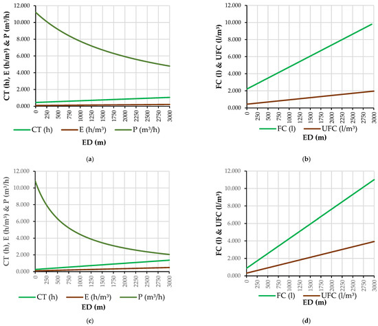
Figure 2.
Cycle time, efficiency, productivity, fuel consumption and unit fuel consumption as a function of extraction distance by considering the average payload size and the number of pieces per load for the skidder (a,b) and farm tractor (c,d) datasets: (a) variation in cycle time, efficiency and productivity for the skidder dataset, (b) variation in fuel consumption and unit fuel consumption for the skidder dataset, (c) variation in cycle time, efficiency and productivity for the farm tractor dataset, (d) variation in fuel consumption and unit fuel consumption for the farm tractor dataset.
In terms of cycle time, the models were comparable within the observed range of extraction distances, with only minor differences indicating a higher cycle time for farm tractors when exceeding an extraction distance of 1000 m. However, the slope of the models for extraction distance differed for the two machines (Table 5), highlighting the impact of other variables on the skidder dataset, particularly at lower ranges of extraction distances. Considering the differences in average payload sizes and the number of pieces per payload, the effects of extraction distance on productivity were contrasting, especially when exceeding approximately 50 m. Beyond this point, the productivity of farm tractors decreased more sharply as a function of extraction distance, reaching only half that of skidders at an extraction distance of about 1500 m. Consequently, skidders became more efficient (Figure 2a,c) at higher extraction distances.
In terms of fuel consumption, the findings were consistent with those related to productivity and efficiency. At comparable fuel consumption levels, farm tractors demonstrated almost double the unit fuel consumption at extraction distances approaching 3000 m, likely as a result of payload size.
4. Discussion
The goal of this study was achieved, as models to predict time and fuel consumption were successfully developed and subsequently used to model and predict efficiency, productivity, and unit fuel use under the average conditions observed in the study. Furthermore, the data used to develop these models is nationally representative, allowing the models to reflect the average operational conditions concerning forest type, tree size, ground conditions, and season of operation. Additionally, our refined datasets included a significant number of work cycles and a diverse range of observed variables, such as extraction distances, payload sizes, and the number of pieces per payload, all of these being relevant for the currently used machines in skidding operations.
However, the assumptions of regression analysis modeling were only partly met. While the assumptions of linearity and absence of multicollinearity were satisfied for all models, the assumptions of multivariate normality (i.e., a normal distribution of residuals) and homoskedasticity (i.e., consistent variance of residuals across all levels of independent variables) were only partially satisfied. Regarding multivariate normality, our results indicated slight deviations from normality in some cases—specifically, in the cycle time and fuel consumption models for the skidder and farm tractors, respectively. We observed a departure from normality in the skidder fuel consumption model, while the farm tractor fuel consumption model exhibited normality of residuals.
Heteroskedasticity can also be present in studies analyzing operational performance, given the high variability in data as the magnitude of predictors, such as extraction distance, increases, due to unaccounted factors. While these factors can be relevant to the predictive power of the developed models, it is often quite difficult, if not impossible, to exercise control over all relevant variables [33]. Furthermore, accounting for too many factors may lead to other issues, such as compromising the accuracy of the study [36]. From this perspective, the cycle time consumption models were affected by slight heteroskedasticity, primarily due to the influence of extraction distance.
Notwithstanding this, the predictions shown in Figure A2 and Figure A3 still indicate a high predictive power of the developed models, particularly when extraction distance and payload volumes are considered as predictors. Indeed, factors such as the ground conditions of the trails, the silvicultural systems implemented, extraction intensity, the season of work, and the personal experience of the work crews are among the recognized factors affecting operational performance [37,38,39]. Therefore, there will always be a trade-off between a model’s predictive power and the factors accounted for in the model. The aim of this study was to offer a general set of models for the country, primarily focused on informing decision-making and depicting the performance of operations at both tactical and strategic levels, which we believe we have achieved. This comes in the context in which the existing rates [31] are obsolete for the machines in use, whereas the existing national data comes only from disparate studies addressing targeted conditions, e.g., [11,21,22,28]. For operational planning, however, other factors need to be accounted for to better reflect the situation in specific harvesting areas concerning forest and trail conditions, worker experience, and season of operation. Such models, however, will always suffer from limited amounts of data used to build them, as well as from low inclusion and quantification of diversity in crew experience.
Skidding models for purpose-built skidders operating in steep terrain consistently identify skidding distance, winching distance, and slope (or trail slope) as the most influential variables for predicting cycle time, productivity, and cost. In a selection cut on a 30% slope using a Timberjack 450C, it was found that these three variables—especially the interaction between skidding distance and slope—were the primary predictors of cycle time [40]. The study reported gross and net productivity rates of 20.51–22.93 m3 h−1 at an average skidding distance of approximately 290 m, with unit costs of 6.31–6.22 USD m−3. Comparatively, Horvat et al. [41] examined the ECOTRAC 120V skidder in hilly (+4% trail) and mountainous (−9.6% trail) conditions, illustrating how steeper and more adverse trails can amplify the effect of distance on time consumption. Travel speeds decreased from 5.69 to 2.20 km h−1 unloaded and from 3.55 to 1.67 km h−1 loaded. Time increased from 10.35 to 12.03 min m−3, and daily output dropped as distances grew, despite downhill loaded travel in the mountainous site [41]. This contrast shows that heavier average loads and adverse trail slopes force operators to reduce travel speed more drastically, thus increasing the time required per cubic meter [40,41]. On gentle terrain (~4.5°) with good trail conditions, the wheel configuration itself may be a significant driver of performance, as demonstrated by [42]. Rubber tires achieved the highest productivity and lowest unit cost at longer extraction distances, while adding tracks improved mobility in weak or steep ground but reduced driving speed and productivity on firm, level trails. The fuel cost share also increased to approximately 29%–32% of the total when tracks were used due to higher rolling resistance. Compared to the steep-slope results from [40,41], on favorable terrain, equipment configuration can outweigh slope as a determinant of productivity and fuel efficiency. In contrast, on steep terrain, slope remains an important factor regardless of wheel type. With these in mind, our study successfully incorporates key variables into the developed models for specialized skidders, including payload volume, number of pieces, and extraction distances. These variables serve as relevant predictors, reflecting the time consumption for pre-skidding with double-drum winches, which involve multiple repetitions to form a payload, as well as the variability in load weights and extraction distances.
For farm tractors, the effect of slope and trail gradient can be even more pronounced. Gilanipoor et al. [25] found that in mountainous forests, a tractor’s delay-free productivity was 2.60 m3 h−1 (2.43 m3 h−1 with delays), with only skidding distance and trail slope emerging as significant predictors of cycle time. They reported sharp declines in performance above a 15% trail slope, recommending that tractors be restricted to longer but gentler skid trails. In contrast, Acar et al. [43], while observing farm tractors working on very steep ground (60% slope) in uphill skidding, recorded an average cycle time of 7.49 min at approximately 95 m skidding distance and a productivity of 8.467 m3 h−1, with winching alone accounting for 31% of cycle time. Under favorable terrain and trail conditions, farm tractors can perform much more competitively. Spinelli & Magagnotti [44] have found that in small-scale forestry operations using a sulky and adequate suspension, tractors could achieve productivity levels above 3 m3 and up to about 8 m3 SMH−1. Their models identified piece size, winching distance, tractor power, skidding distance, and crew size as significant predictors. Fossil energy consumption ranged from 50 to 100 MJ m−3 (about 1.3–2.7 L diesel m−3), and extraction costs could be reduced to below EUR 10 m−3 when working on lowland sites with good trails, large piece sizes, and short winching distances. Compared to the steep terrain cases of [25,43], these results emphasize how favorable site and trail conditions, combined with appropriate equipment configuration, can transform tractor productivity and fuel efficiency, and our study indicates a similar performance for farm tractors when working on gentle slopes.
Overall, the literature indicates that for skidders, core predictive variables across models include skidding and winching distance, slope (or trail slope), and load size, with equipment configuration (wheels vs. tracks) also being relevant in favorable terrain. For farm tractors, key variables such as skidding and winching distance, piece or load size, power, and trail slope dominate model structures. Steep or adverse trails impose significant performance penalties, while gentle, well-maintained trails facilitate competitive productivity, efficiency, and fuel consumption. Comparisons between authors highlight that while skidders generally outperform tractors in steep and complex terrain, tractors can rival or even exceed skidder efficiency in lowland or gently sloped conditions with good trails.
As the technology progresses, long-term operational data may be sourced by other techniques that integrate GNSS tracking. Machine learning has already progressed substantially and has shown a high potential for classification tasks based on sensor data [45,46,47], which, coupled with improved GNSS tracking [48,49], can offer a solution also for commonly used cable skidders and farm tractors that lack data collection capabilities. Moreover, computer vision techniques were found lately to be highly performant in activity recognition. Such techniques could probably solve the problem of long-term data collection, processing, and analysis, providing valuable tools to improve our understanding on operational performance. This will enhance our ability to run automated time studies by advancing already used techniques [50,51,52,53].
5. Conclusions
This study developed updated models to estimate cycle time and fuel consumption for double-drum winch skidders and single-drum winch agricultural tractors adapted for skidding, using a nationally representative all-season dataset. The models incorporate key variables such as extraction distance, payload volume, and the number of pieces per cycle, which enable the characterization and differentiation of both machine types under diverse operational conditions in Romania. For skidders, variability in cycle time and fuel consumption is primarily explained by the combined effects of extraction distance, payload volume, and number of pieces. In contrast, for agricultural tractors, extraction distance is the only significant predictor, indicating lower sensitivity to load characteristics. Simulations reveal that at short extraction distances, productivity differences are minor; however, beyond 50 m, farm tractors lose competitiveness, achieving only half the productivity of skidders at approximately 1500 m, along with a notable increase in unit fuel consumption. These results provide a reliable tool for planning skidding operations and offer a scientific basis for comparing machines and guiding decisions on their allocation based on working conditions. However, for a better fit and application in more localized contexts, the models should be adjusted to include specific factors such as slope, trail conditions, forest type, equipment configuration, and crew experience. Additionally, the study emphasizes the need for developing automated methods and systems for long-term performance assessment, which would enhance the accuracy and timeliness of the models, as well as their ability to reflect the technological evolution of machines and timber harvesting practices.
Author Contributions
Conceptualization, S.A.B.; methodology, S.A.B.; validation, M.C.Z.V. formal analysis, M.C.Z.V.; investigation, M.C.Z.V.; resources, S.A.B.; data curation, S.A.B.; writing—original draft preparation, S.A.B. and M.C.Z.V.; writing—review and editing, S.A.B. and M.C.Z.V.; visualization, S.A.B. and M.C.Z.V.; supervision, S.A.B.; project administration, S.A.B.; funding acquisition, S.A.B. All authors have read and agreed to the published version of the manuscript.
Funding
This research was funded mainly by the National Forest Administration—RNP Romsilva, grant number 4522/14.05.2020, which provided the resources for field data collection. The APC of this study was waived. Part of this work was supported by two grants of the Romanian Ministry of Education and Research, CNCS—UEFISCDI, project number PN-IV-P8-8.1-PRE-HE-ORG-2023-0141, and project number PN-IV-P8-8.1-PRE-HE-ORG-2024-0186, within PNCDI IV, which supported part of the methods, data storage and the computing resources used in this study.
Data Availability Statement
The main data, models and statistics are included in this paper. The database may be released upon a reasonable request to the corresponding author of the study.
Acknowledgments
The authors acknowledge the support of forest regional directorates selected as study areas and to the National Forest Administration—RNP Romsilva for the logistical support during field data collection.
Conflicts of Interest
The authors declare no conflicts of interest.
Appendix A


Figure A1.
Examples for the time consumption categories described in Table 2, as collected by the video cameras: (a) driving to the pre-skidding site with a cable skidder, (b) driving with the payload to the forest road with a cable skidder, (c) pulling in the payload with a cable skidder, (d) maneuvering and bunching at the forest road with a cable skidder, (e) driving to the pre-skidding site with a farm tractor, (f) driving with the payload to the forest road with a farm tractor, (g) pulling out the cable from a farm tractor, (h) maneuvering and bunching at the forest road with a farm tractor.


Figure A2.
Supporting data for the cycle time consumption model of skidder dataset: (a) normal probability plot of the CT variable, (b) line fit plot of CT based on ED variable, (c) line fit plot of CT based on NP variable, (d) line fit plot of CT based on PV variable, (e) residual plot of ED variable, (f) residual plot of NP variable, (g) residual plot of PV variable, (h) boxplot of model’s residuals, and (i) histogram of model’s residuals.


Figure A3.
Supporting data for the cycle time consumption model of farm tractor dataset: (a) normal probability plot of the CT variable, (b) line fit plot of CT based on ED variable, (c) line fit plot of CT based on PV variable, (d) residual plot of ED variable, (e) residual plot of PV variable, (f) boxplot of model’s residuals, and (g) histogram of model’s residuals.
References
- Lundbäck, M.; Häggström, C.; Nordfjell, T. Worldwide trends in methods for harvesting and extracting industrial roundwood. Int. J. For. Eng. 2021, 32, 202–215. [Google Scholar] [CrossRef]
- Spinelli, R.; Magagnotti, N.; Visser, R.; O’Neal, B. A survey of skidder fleet of Central, Eastern and Southern Europe. Eur. J. For. Res. 2021, 140, 901–911. [Google Scholar] [CrossRef]
- Oprea, I. Tehnologia Exploatări Lemnului; Transilvania University Press: Brasov, Romania, 2008; pp. 11–17. [Google Scholar]
- Neruda, J.; Nevrkla, P.; Staněk, L.; Zemánek, T. Tractors and Skidders in Forestry; Mendelova University v Brně: Brno, Czech Republic, 2023. [Google Scholar]
- Nikooy, M.; Ahrari, S.; Salehi, A.; Naghdi, R. Effects of rubber-tired skidder and farm tractor on physical properties of soil in plantation areas in the north of Iran. J. For. Sci. 2015, 61, 393–398. [Google Scholar] [CrossRef]
- Erler, J.; Spinelli, R.; Borz, S.A.; Mederski, P.S. Technodiversity in Forest Operations; Transilvania University Press: Brasov, Romania, 2023; pp. 4–88. [Google Scholar]
- Marchi, E.; Chung, W.; Visser, R.; Abbas, D.; Nordfjell, T.; Mederski, P.S.; McEwan, A.; Brink, M.; Laschi, A. Sustainable Forest Operations (SFO): A new paradigm in a changing world and climate. Sci. Total Environ. 2018, 634, 1385–1397. [Google Scholar] [CrossRef] [PubMed]
- Palander, T.; Haavikko, H.; Kortelainen, E.; Kärhä, K.; Borz, S.A. Improving environmental and energy efficiency in wood transportation for a carbon-neutral forest industry. Forests 2020, 11, 1194. [Google Scholar] [CrossRef]
- Kopseak, H.; Šušnjar, M.; Bačić, M.; Šporčić, M.; Pandur, Z. Skidders fuel consumption in two different working regions and types of forest management. Forests 2021, 12, 547. [Google Scholar] [CrossRef]
- Holzleitner, F.; Stampfer, K.; Visser, R. Utilization rates and cost factors in timber harvesting based on long-term machine data. Croat. J. For. Eng. 2011, 32, 501–508. [Google Scholar]
- Borz, S.A.; Mariş, A.C.; Kaakkurivaara, N. Performance of skidding operations in low-access and low-intensity timber removals: A simulation of productivity and fuel consumption in mature forests. Forests 2023, 14, 265. [Google Scholar] [CrossRef]
- Klvac, R.; Skoupy, A. Characteristic fuel consumption and exhaust emissions in fully mechanized logging operations. J. For. Res. 2009, 14, 328–334. [Google Scholar] [CrossRef]
- Heinimann, H.R. A computer model to differentiate skidder and cable-yarder based road network concepts on steep slopes. J. For. Res. 1998, 3, 1–9. [Google Scholar] [CrossRef]
- Ryan, T.; Phillips, H.; Ramsay, J.; Dempsey, J. Forest Road Manual: Guidelines for the Design, Construction and Management of Forest Roads; COFORD: Dublin, Ireland, 2004; pp. 1–155. [Google Scholar]
- Björheden, R.; Apel, K.; Shiba, M.; Thompson, M. IUFRO Forest Work Study Nomenclature; Department of Operational Efficiency, Swedish University of Agricultural Science: Grapenberg, Sweden, 1995; 16p. [Google Scholar]
- Visser, R.; Spinelli, R. Determining the shape of the productivity function for mechanized felling and felling-processing. J. For. Res. 2011, 17, 397–402. [Google Scholar] [CrossRef]
- Ackerman, P.; Belbo, H.; Eliasson, L.; De Jong, A.; Lazdins, A.; Lyons, J. The COST model for calculation of forest operation costs. Int. J. For. Eng. 2014, 25, 75–81. [Google Scholar] [CrossRef]
- Proto, A.R.; Macri, G.; Visser, R.; Russo, D.; Zimbalatti, G. Comparison of timber extraction productivity between winch and grapple skidding: A case study in Southern Italian Forests. Forests 2018, 9, 61. [Google Scholar] [CrossRef]
- Gülci, S.; Büyüksakalli, H.; Taş, I.; Akay, A.E. Productivity analysis of timber skidding operation with farm tractor. Eur. J. For. Eng. 2018, 4, 26–32. [Google Scholar] [CrossRef][Green Version]
- Özturk, T.; Varsak, M.G.; Bilici, E. Evaluating productivity and cycle time of skidding method with farm tractors in Bigadic Forest Enterprise Directorate in Turkey. Eur. J. For. Eng. 2018, 5, 77–82. [Google Scholar] [CrossRef]
- Borz, S.A.; Ignea, G.; Popa, B.; Sparchez, G.; Iordache, E. Estimating time consumption and productivity of roundwood skidding in group shelterwood system—A case study in a broadleaved mixed stand located in reduced accessibility conditions. Croat. J. For. Eng. 2015, 36, 137–146. [Google Scholar]
- Borz, S.A.; Dinulica, F.; Birda, M.; Ignea, G.; Ciobanu, V.D.; Popa, B. Time consumption and productivity of skidding Silver fir (Abies alba Mill.) round wood in reduced accessibility conditions: A case study in windthorw salvage logging from Romanian Carpathians. Ann. For. Res. 2013, 56, 363–375. [Google Scholar]
- Sowa, J.M.; Szewczyk, G. Time consumption of skidding in mature stands performed by winches powered by farm tractor. Croat. J. For. Eng. 2013, 34, 255–264. [Google Scholar]
- Gallis, C.; Spyroglou, G. Productivity linear regressions of tree-length harvesting system in natural coastal Aleppo pine (Pinus halepensis L.) forests in the Chalkidiki area of Greece. Croat. J. For. Eng. 2012, 33, 115–123. [Google Scholar]
- Gilanipoor, N.; Najafi, A.; Heshmat Alvaezin, S.M. Productivity and cost of farm tractor skidding. J. For. Sci. 2012, 58, 21–26. [Google Scholar] [CrossRef]
- Sabo, A.; Poršinsky, T. Skidding of fir roundwood by Timberjack 240C from selective forests of Groski Kotar. Croat. J. For. Eng. 2005, 26, 13–27. [Google Scholar]
- Vusić, D.; Šušnjar, M.; Marchi, E.; Spina, R.; Zečić, Ž.; Picchio, R. Skidding operations in thinning and shelterwood cut of mixed stands—Work productivity, energy inputs and emissions. Ecol. Eng. 2013, 61, 216–223. [Google Scholar] [CrossRef]
- Borz, S.A.; Mititelu, V.-B. Productivity and Fuel Consumption in Skidding Roundwood on Flat Terrains by a Zetor Farm Tractor in Group Shelterwood Cutting of Mixed Oak Forests. Forests 2022, 13, 1294. [Google Scholar] [CrossRef]
- Hiesl, P.; Benjamin, J.G. Applicability of international harvesting equipment productivity studies in Maine, U.S.A.: A literature review. Forests 2013, 4, 898–921. [Google Scholar] [CrossRef]
- Moskalik, T.; Borz, S.A.; Dvorák, J.; Ferencik, M.; Glushkov, S.; Muiste, P.; Lazdinš, A.; Styranivsky, O. Timber harvesting methods in Eastern European countries: A review. Croat. J. For. Eng. 2017, 38, 231–241. [Google Scholar]
- Ministry of Timber Industrialization and Construction Materials. Norme şi Normative de Muncă Unificate în Exploatări Forestiere; 1989; p. 493. [Google Scholar]
- Athanassiadis, D.; Lideslav, G.; Wasterlund, I. Fuel, hydraulic oil and lubricant consumption in Swedish mechanized harvesting operation. Int. J. For. Eng. 1999, 10, 59–66. [Google Scholar]
- Acuna, M.; Bigot, M.; Guerra, S.; Hartsough, B.; Kanzian, C.; Kärhä, K.; Lindroos, O.; Magagnotti, N.; Roux, S.; Spinelli, R.; et al. Good Practice Guidelines for Biomass Production Studies; CNR IVALSA Sesto Fiorentino (National Research Council of Italy—Trees and Timber Institute): Sesto Fiorentino, Firenze, Italy, 2012; 52p. [Google Scholar]
- Heinimann, H.R. Operational Productivity Studies in Forestry Based on Statistical Models. ETH Forest Engineering Research Paper. 2021. Available online: https://www.researchgate.net/publication/349636743_Operational_Productivity_Studies_in_Forestry_Based_on_Statistical_Models_-_A_Tutorial (accessed on 1 July 2025).
- Real Statistics Using Excel. Available online: https://real-statistics.com/ (accessed on 18 July 2025).
- Spinelli, R.; Laina-Relano, R.; Magagnotti, N.; Tolosana, E. Determining observer and method effects on the accuracy of elemental time studies in forest operations. Balt. For. 2013, 19, 301–306. [Google Scholar]
- Grzywiński, W.; Turowski, R.; Naskrent, B.; Jelonek, T.; Tomczak, A. The Impact of Season on Productivity and Time Consumption in Timber Harvesting from Young Alder Stands in Lowland Poland. Forests 2020, 11, 1081. [Google Scholar] [CrossRef]
- Melander, L.; Ritala, R. Separating the impact of work environment and machine operation on harvester performance. Eur. J. For. Res. 2020, 139, 1029–1043. [Google Scholar] [CrossRef]
- Kluender, R.; Lortz, D.; McCoy, W.; Stokes, B.; Klepac, J. Removal intensity and tree size effects on harvesting cost and profitability. For. Prod. J. 1998, 48, 54–59. [Google Scholar]
- Behjou, F.K.; Majnounian, B.; Namiranian, M.; Dvořák, J. Time study and skidding capacity of the wheeled skidder Timberjack 450C in Caspian forests. J. For. Sci. 2008, 54, 183–188. [Google Scholar] [CrossRef]
- Horvat, D.; Zečić, Ž.; Šušnjar, M. Morphological characteristics and productivity of skidder ECOTRAC 120V. Croat. J. For. Eng. 2007, 28, 11–25. [Google Scholar]
- Lopes, E.D.S.; Oliveira, D.D.; Sampietro, J.A. Influence of wheeled types of a skidder on productivity and cost of the forest harvesting. Floresta 2014, 44, 53–62. [Google Scholar] [CrossRef]
- Acar, H.H.; Kaya, A.; Ünver-Okan, S.; Üçüncü, K. Evaluation of Skidding System by MB Trac 900 Forest Tractors on Steep Slopes in Thinning Operations; University of Natural Resources and Life Sciences: Vienna, Austria, 2015; pp. 381–383. [Google Scholar]
- Spinelli, R.; Magagnotti, N. Wood extraction with farm tractor and sulky: Estimating productivity, cost and energy consumption. Small-Scale For. 2012, 11, 73–85. [Google Scholar] [CrossRef]
- Borz, S.A.; Proto, A.R. Predicting Operational Events in Mechanized Weed Control Operations by Offline Multi-Modal Data and Machine Learning Provides Highly Accurate Classification in Time Domain. Forests 2024, 15, 2019. [Google Scholar] [CrossRef]
- Keefe, R.F.; Zimbelman, E.G.; Wempe, A.M. Use of smartphone sensors to quantify the productive cycle elements of hand fallers on industrial cable logging operations. Int. J. For. Eng. 2019, 30, 132–143. [Google Scholar] [CrossRef]
- Zimbelman, E.G.; Keefe, R.F. Development and validation of smartwatch-based activity recognition models for rigging crew workers on cable logging operations. PLoS ONE 2021, 16, e0250624. [Google Scholar] [CrossRef]
- Keefe, R.F.; Wempe, A.M.; Becker, R.M.; Zimbelman, E.G.; Nagler, E.S.; Gilbert, S.L.; Caudill, C.C. Positioning Methods and the Use of Location and Activity Data in Forests. Forests 2019, 10, 458. [Google Scholar] [CrossRef]
- Keskin, M.; Say, S.M. Feasibility of low-cost GPS receivers for ground speed measurement. Comp. Elect. Agric. 2006, 54, 36–43. [Google Scholar] [CrossRef]
- Contreras, M.; Freitas, R.; Ribeiro, L.; Stringer, J.; Clark, C. Multi-camera surveillance systems for time and motion studies of timber harvesting equipment. Comp. Elect. Agric. 2017, 135, 208–215. [Google Scholar] [CrossRef]
- McDonald, T.P.; Fulton, J.P. Automated time study of skidders using global positioning system data. Comp. Elect. Agric. 2005, 48, 19–37. [Google Scholar] [CrossRef]
- Bacescu, N.M.; Piol, O.; Talbot, B.; Marchi, L.; Grigolato, S. Modelling full stems skidding in northeast Italian Alps through engine data acquisition and analysis. Eur. J. For. Res. 2025, 1–12. [Google Scholar] [CrossRef]
- Mologni, O.; Lahrsen, S.; Roeser, D. Automated production time analysis using FPDat II onboard computers: A validation study based on whole-tree ground-based harvesting operations. Comput. Electron. Agric. 2024, 222, 109047. [Google Scholar] [CrossRef]
Disclaimer/Publisher’s Note: The statements, opinions and data contained in all publications are solely those of the individual author(s) and contributor(s) and not of MDPI and/or the editor(s). MDPI and/or the editor(s) disclaim responsibility for any injury to people or property resulting from any ideas, methods, instructions or products referred to in the content. |
© 2025 by the authors. Licensee MDPI, Basel, Switzerland. This article is an open access article distributed under the terms and conditions of the Creative Commons Attribution (CC BY) license (https://creativecommons.org/licenses/by/4.0/).