Initial Insights into Spruce Wood Fatigue Behaviour Using Dynamic Mechanical Properties in Low-Cycle Fatigue

Abstract

Damaged material invariably exhibits a lower resonance frequency than undamaged material due to its reduced stiffness. Under fatigue loading, damage accumulates until failure, so changes in resonance frequency can be utilised as a variable to predict fatigue life. Conventional fatigue life prediction methods have a low success rate, prompting the exploration of alternative approaches. We have presented a novel method for predicting the fatigue life of spruce wood based on changes in resonance frequency during fatigue, using a representative specimen (i.e., one out of five specimens tested, with four used for static strength reference). We conducted a low-cycle fatigue test and monitored the resonance frequency alongside the dynamic and static modulus of elasticity. All three types of data were employed to predict fatigue life using between 40% and 100% of the measurement data. Of the two fatigue life prediction methods investigated, the Weibull cycle density distribution using resonance frequency measurements proved most appropriate. The error decreases monotonically with the amount of resonance frequency measurement data used for fatigue life prediction, reaching its lowest value of 1% when the full resonance frequency dataset is used. The proposed fatigue life prediction method should be further validated with a larger sample size, as fatigue is inherently a statistical phenomenon.

1. Introduction

The properties of undamaged and damaged materials in terms of resonance frequency have been extensively researched through review [1], beam damage assessments [2], damage identification studies [3], evaluations of mechanical properties [4] and investigations of resonance frequency changes [5,6,7]. A common finding is that undamaged materials exhibit higher resonance frequencies than damaged materials due to their greater stiffness. Material fatigue, resulting from the accumulation of damage, leads to a progressive reduction in stiffness and ultimately to failure. Consequently, the resonance frequency of a material is frequently used as a key parameter for monitoring its condition and predicting the development of fatigue damage. Modal analysis has already demonstrated its utility in studying the fatigue of steel [8,9,10], aluminium alloys [11] and composite materials [12,13,14]; however, research in this area is less developed for wood.

For wood exhibiting complex anisotropic properties, predicting the time to failure using conventional methods is less successful, as noted by Šraml [15] in a review of wood fatigue life models. Multiple studies by Klemenc [16,17] indicate low predictive success due to small test populations. Others have highlighted a lack of generalisation in current wood fatigue life prediction models [18,19]. Wood is a natural composite material whose mechanical properties strongly depend on its internal structure, including the orientation and distribution of fibres and moisture content [20]. Previous research has demonstrated that cracks and lower density in wood affect resonance frequency and damping [5,21]. Modal analysis has been successfully employed to predict the development of fatigue damage in glued joints [22] and polymer composites [23], suggesting the potential of this approach for studying wood. While the Weibull distribution has been used to model fatigue in metallic and composite systems [24], its application in resonance-based fatigue monitoring for wood has not yet been reported.

Existing studies have focused on changes in modal parameters during the fatigue of materials such as concrete, metals, and composites [25,26]. These studies have found that a decrease in resonance frequency correlates with the accumulation of damage and the growth of cracks, enabling real-time monitoring of material condition. For example, the study by Bedewi [23] demonstrated that resonance frequency is a reliable indicator of crack growth in polymer composites; however, similar studies are scarce for wood-based materials. Divós [27] found that the correlation between the static and dynamic properties of wood could be useful for estimating creep, but further research is required to enhance robustness. Low-cycle fatigue refers to fatigue conditions in which materials are subjected to a relatively small number of load cycles (typically fewer than ${10}^4$), usually at high stress levels [10,28].

The aim of this study was to develop a method for monitoring the dynamic properties of spruce wood under low-cycle fatigue and to evaluate the usefulness of modal parameters in predicting fatigue life. By investigating changes in resonance frequency and modulus of elasticity, we sought to determine whether it is possible to accurately predict the number of cycles to failure based on early measurements. This approach could make a significant contribution to the development of methods for monitoring the condition of timber structures and enhancing their safety and durability under real-world conditions.

2. Theory of Calculations

2.1. Dynamic Material Properties

The dynamic material properties during bending vibrations include the dynamic modulus of elasticity, which depends on the resonance frequency, the cross-sectional area, and the density of the sample. To calculate the dynamic modulus of elasticity for the fundamental mode of vibration, we used the Euler–Bernoulli solution expressed by the differential Equation (1) for the free vibration of a beam [29,30]. Despite the anisotropic nature of wood, the Euler–Bernoulli theory provides sufficiently accurate results for slender beams under bending, particularly in the first mode of vibration [31,32].

$${\displaystyle \frac{{\partial }^{2}w}{\partial t^2}}=-c^2{\displaystyle \frac{{\partial }^{4}w}{\partial x^4}}$$

(1)

where w is a product of the spatial $u\left(x\right)$ and the time function $q\left(t\right)$, written as follows:

$$w=u\left(x\right)·q\left(t\right)$$

(2)

and c is calculated as follows:

$$c=\sqrt{{\displaystyle \frac{EI}{\rho A}}}$$

(3)

E is the elastic modulus, I is the area moment of inertia, $\rho$ is the material density, and A is the cross-sectional area. After substituting Equation (2) into Equation (1) and considering the boundary conditions of a free beam—namely that the shear stress and bending moment are zero, written as follows:

$$\begin{array}{c}\hfill u^{″}\left(0\right)=0,u^{″}\left(L\right)=0\\ \hfill u^{‴}\left(0\right)=0,u^{‴}\left(L\right)=0\end{array}$$

(4)

we derive the frequency equation for the free vibration of a beam, written as follows:

$$cos\left(kL\right)cos\left(kL\right)=1$$

(5)

where k is calculated as follows:

$$k=\sqrt{{\displaystyle \frac{\omega }{c}}}$$

(6)

The first solution of Equation (6) is $k_{1}L=4.73$. Solving Equation (1) for the function $u\left(x\right)$ of the spatially dependent vibration, we obtain the following:

$$w_1\left(x\right)=\left[sinh\left({\displaystyle \frac{k_{1}L}{L}}x\right)+sin\left({\displaystyle \frac{k_{1}L}{L}}x\right)\right]+{\displaystyle \frac{sin\left(k_{1}L\right)-sinh\left(k_{1}L\right)}{cosh\left(k_{1}L\right)-cos\left(k_{1}L\right)}}\left[cosh\left({\displaystyle \frac{k_{1}L}{L}}x\right)+\cos \left({\displaystyle \frac{k_{1}L}{L}}x\right)\right]$$

(7)

We measured the resonance frequency of the first mode of vibration using the method described in the literature [31]. The selected frequency range, centred around the first bending mode (≈600 Hz), was chosen to ensure optimal sensitivity to stiffness degradation while minimising attenuation effects. This mode is particularly effective for clear wood samples of the given dimensions, as it provides a high signal-to-noise ratio and a stable modal response. Previous studies have demonstrated that this frequency range is appropriate for vibration-based damage detection in wood and composite beams [2,4]. We positioned the supports at a distance from the edge of the specimen so that the nodal points of the wave coincide precisely with the support points (Figure 1). This arrangement minimises, the damping of the vibration. The positions of the supports can be calculated once the solution to Equation (8) has been obtained.

$$w_1\left(x\right)=0$$

(8)

The relative distance of the supports from the edge of the beam is $x_1=0.224$ and $x_2=0.776$ for a simply supported beam in the first mode of vibration.

Considering the Equations (9) and the Equation (6) we can conclude the following:

$${\omega }_1=k_1^{2}c={\displaystyle \frac{{\left(k_{1}L\right)}^2}{L^2}}\sqrt{{\displaystyle \frac{EI}{\rho A}}}$$

(9)

and derive the Equation (10) of the dynamic modulus of elasticity.

$$E_d={\displaystyle \frac{{\omega }_1^2·L^4·\rho ·A}{{\left(k_{1}L\right)}^4·I}}={\displaystyle \frac{{\left(2\pi f_1\right)}^2·L^4·\rho ·A}{{\left(k_{1}L\right)}^4·I}}$$

(10)

2.2. Static Material Properties

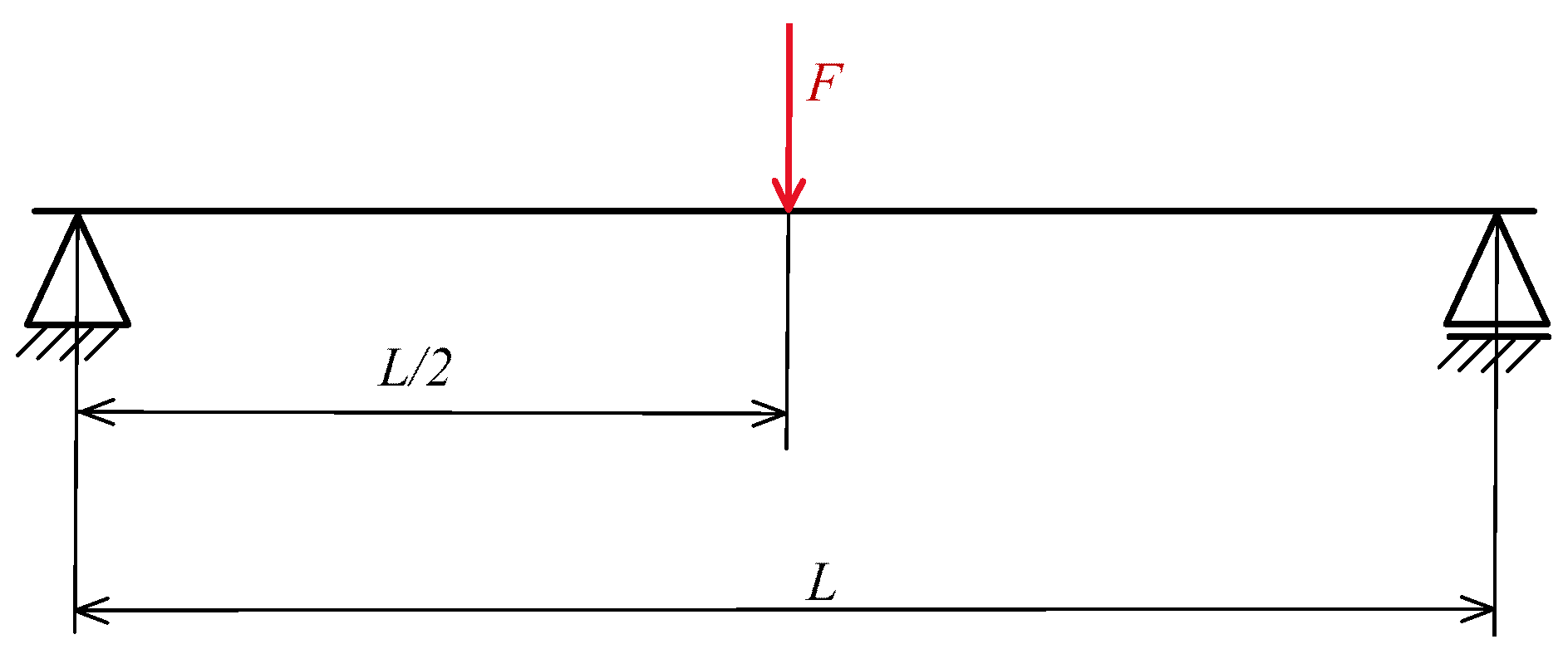
We have calculated the static modulus of elasticity using the deflection Equation (11) for a simply supported beam subjected to a force F at mid-span, as illustrated in Figure 2.

$$E_s={\displaystyle \frac{F·L^3}{48·I·w}}$$

(11)

The maximum stress in three-point bending is calculated from the maximum moment and the section modulus of the cross-section. Equation (12) presents the expression for calculating the stress based on the applied force and the specimen’s geometry.

$$\sigma ={\displaystyle \frac{3·F·L}{2·b·h^2}}$$

(12)

2.3. Weibull Cycle Density Distribution

From all the predicted numbers of cycles to failure, we predicted the fatigue life of the tested specimen using only a portion of the data, applying the Weibull cycle density distribution (c.d.d.). The objective was to determine the number of cycles to failure as accurately as possible from minimal data or cycles. After each new cycle, we obtained a new prediction based on the drop in frequency; these predictions were then statistically analysed using the Weibull c.d.d. as described in Equation (13) [33]. The parameters $\beta$ and $\theta$ of the Weibull c.d.d. were determined using Benard’s approximation [34]. For this approximation, it is necessary to index the predicted number of cycles with the index i and calculate the median rank $P_i$ according to Equation (14). In this equation, $n_i$ represents the total number of predictions. The predicted values must be sorted from the smallest to the largest value $N_s$, and then a linear regression must be performed to find the linear curve that best fits the data. The points X and Y are calculated according to Equation (15). The parameters of the linear curve equation k and n are used to determine the parameters of the Weibull c.d.d. $\beta$ and $\theta$ according to Equation (16).

$$f\left(N\right)={\displaystyle \frac{\beta }{\theta }}{\left({\displaystyle \frac{N}{\theta }}\right)}^{\beta -1}{e}^{-{(N/\theta )}^{\beta }}$$

(13)

$$P_i={\displaystyle \frac{i-0.3}{n_i+0.4}}$$

(14)

$$\begin{array}{c}\hfill X=ln(-ln(1-P_i))\\ \hfill Y=ln\left(N_s\right)\end{array}$$

(15)

$$\begin{array}{c}\hfill \beta =k\\ \hfill \theta =e^{-{\displaystyle \frac{n}{k}}}\end{array}$$

(16)

3. Research Methodology

The test was conducted using a Zwick 1464 mechanical universal testing machine (ZwickRoell GmbH, Ulm, Germany). It was adapted for fatigue testing by incorporating a unit to control the dynamic mechanical excitation (PCI-6024E; National Instruments, Austin, TX, USA) and to record the response signal (PCB-130E20; PCB Piezotronics, Walden, NY, USA). The loading cycle, mechanical excitation, and response signal recording were automated to ensure the most consistent test conditions possible. The data obtained on force, deflection, and resonance frequencies were used to compare the dynamic and static modulus of elasticity and to predict fatigue life.

3.1. Experiment Preparation

The distance between the supports was adjusted according to the length of the specimen. We used clear spruce (P. abies) wood samples measuring 380 mm in length with a cross-section of 15 × 15 mm. Four specimens were employed to determine the static bending strength, while one specimen was used as an example for the fatigue life prediction method proposed in this study. The specimens for both static and dynamic tests were stored for one month under standard conditions at 20 °C and 65% relative humidity. The mean moisture content of all specimens was 12.8% with a coefficient of variation of 3.5%. The moisture content of the fatigue specimen was 13%. These values comply with the standard conditioning procedures outlined in ISO 3129 [35]. The mean density of all specimens was 416.4 kg/m³ and 430.5 kg/m³ for the fatigue specimen. The coefficient of variation of density was 9.3%.

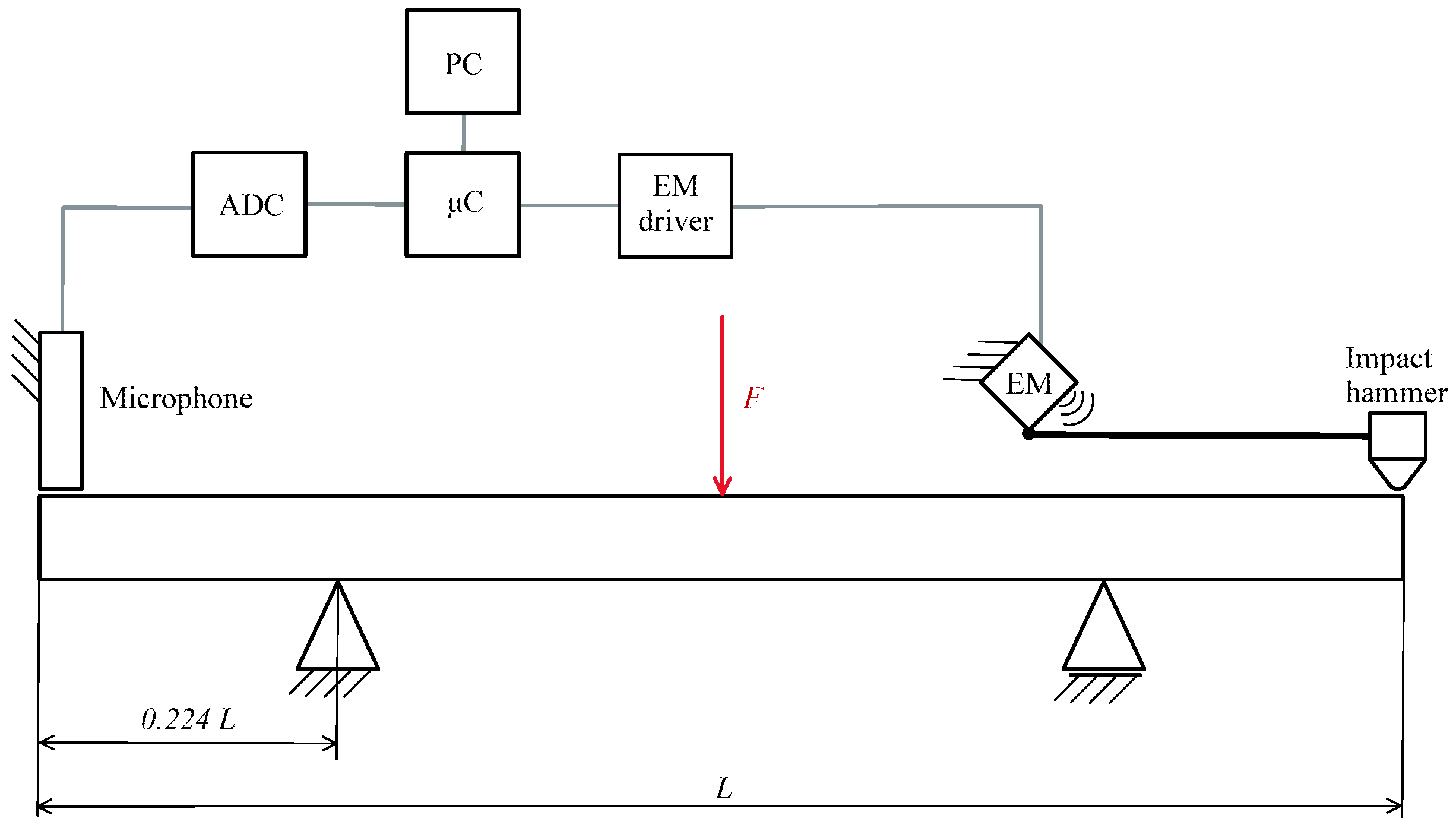
The first vibration mode was determined using the expression $k_{1}L=4.73$, which was used to calculate the distance between the supports as 210 mm. A schematic of the experimental setup is shown in Figure 3. The main preparations for the test involved modifying the control software of the testing device to perform fatigue tests and integrating the recording of mechanical excitation and the vibration response of the test specimen. The programme was developed in the LabVIEW programming environment.

Cyclic loading with a dynamic load ratio of 0 was applied using a universal testing machine by activating the servomotor drive and the electromagnetic clutch. The loading direction was controlled by the rotation of the servomotor and changed (1) when the preset loading force was reached, and (2) when the preset home position was attained without applying load to the specimen.

For each loading cycle, once the loading tool had reached the starting position and the specimen was unloaded, mechanical excitation was applied to the specimen’s free end. A small wooden hammer, driven by an electromagnet, was used for this purpose. Simultaneously, the response signal was recorded using a microphone attached to the opposite end of the specimen. The response signal was recorded for 1.1 s and was used to determine the resonance frequency of the specimen’s first vibration mode via fast Fourier transformation. The subsequent loading cycle then commenced.

3.2. Experiment Procedure

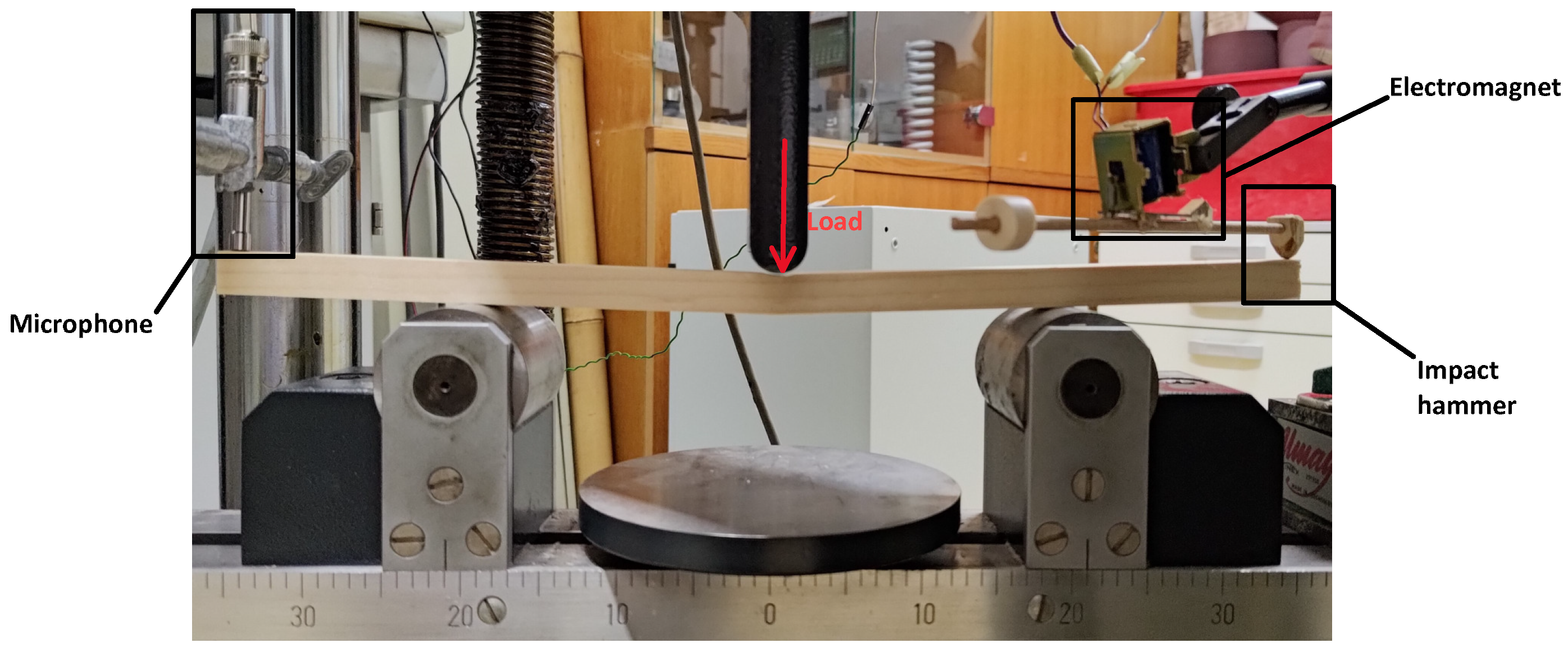
Before the static and fatigue tests, the specimens were weighed, and their thickness and width were measured at the load point. Prior to conducting the cyclic fatigue test, static bending tests were performed to determine the specimens’ static bending strength. The mean static bending strength was 82.5 MPa with a coefficient of variation of 10.6%. For the low-cycle fatigue tests, the maximum force was set to 800 N, corresponding to 90% of the mean static bending strength. The value of 90% was selected based on preliminary tests to ensure low-cycle fatigue behaviour, as described in the literature on the fracture of brittle wood during cyclic bending [15,16] and on stiffness changes during fatigue loading [36]. The force sensor was calibrated, and the starting position was set to approximately 1 mm above the specimen. The microphone and hammer were positioned at an appropriate distance from the specimen surface, as illustrated in Figure 4.

We activated the control software and commenced cyclic loading at a rate of 10 mm/min in both directions. The test was conducted at a frequency of approximately 0.015 Hz. After each cycle, we checked the distance between the hammer, the microphone, and the specimen surface, readjusting as necessary. This was required because the distance between the microphone or hammer and the specimen decreased after several cycles due to plastic deformation. The test concluded when the specimen’s strength had diminished to the point that it could no longer withstand the specified load and failed completely.

3.3. Data Analysis

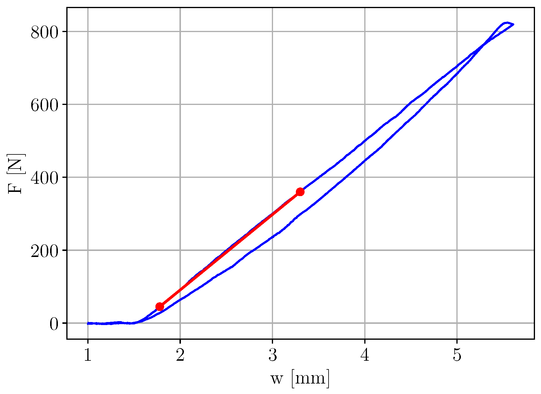
After the fatigue test, we extracted data from each cycle of all recorded cycles for individual analysis. For each loading cycle, we determined the static modulus of elasticity by using the linear portion of the load–deflection curve between 5% and 45% of the maximum load. Due to limitations of the equipment used for static bending strength testing, we employed the three-point bending method and accounted for the size of the indentation caused by local plastic compression deformation under bending load, which is relatively large in spruce wood. The measured indentation at the end of the fatigue test was approximately 1 mm, and we assume this indentation occurred during the initial cycles. The calculated values of the static and dynamic modulus of elasticity, as well as resonance frequencies, were approximated using linear and cubic fitting methods.

We predicted fatigue life using a linear approximation for each segment of the data. We began with the first three values and calculated the predicted number of cycles based on the slope of the linear approximation, the initial values, and the limit values. With each additional data point, both the slope of the approximation and the predicted fatigue life were updated. For the limit values, we selected the lowest values of the modulus of elasticity and resonance frequency derived from the linear approximation. We used the predicted number of cycles at various points in the data to predict the specimen’s fatigue life. Three different approaches were employed: in the simpler methods, the average number of cycles was calculated, and the number of cycles was determined from the slope of the linear approximation at a specific portion of the data; in the more complex approach, the Weibull cycle density distribution was utilised.

4. Results

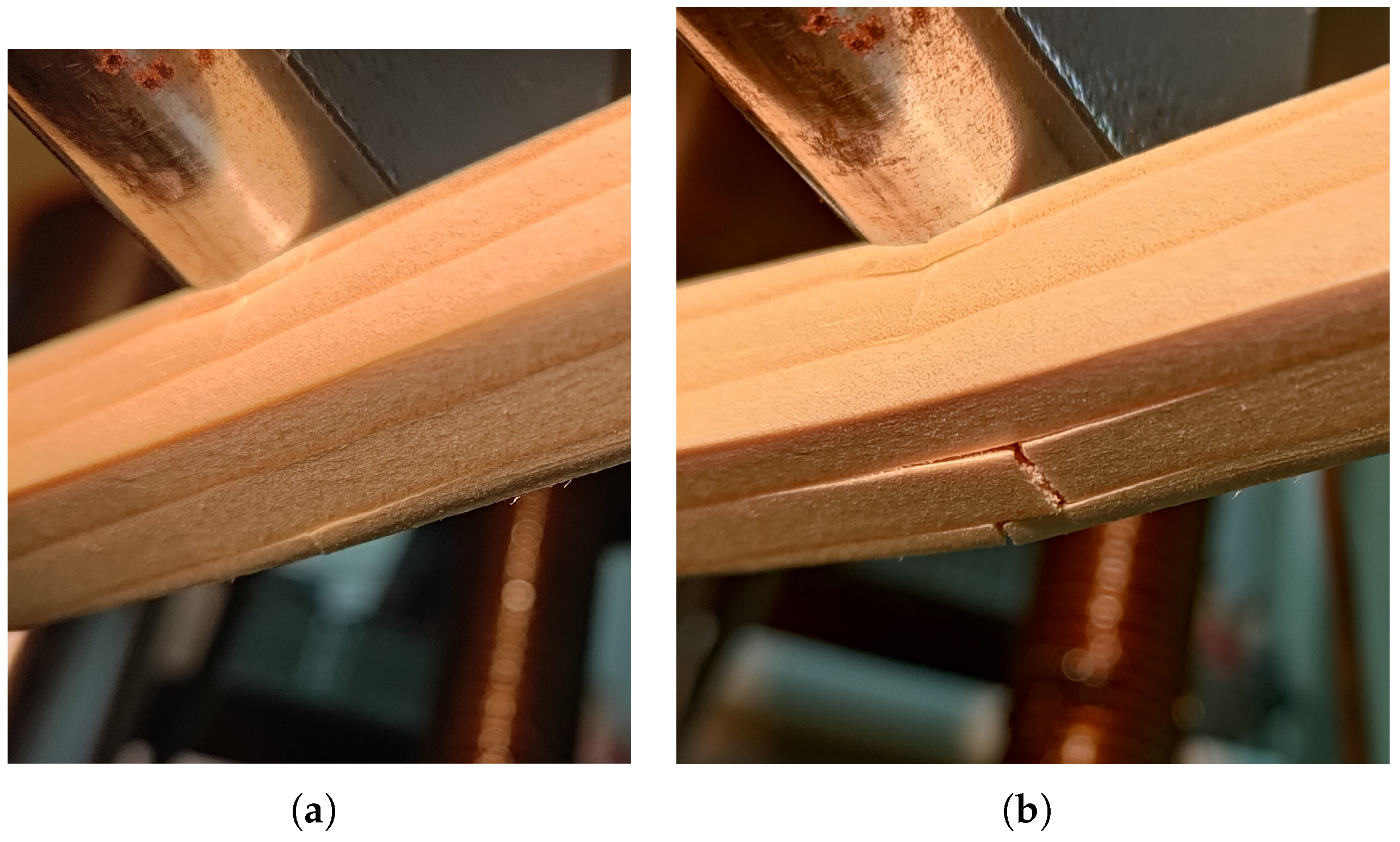
With a cyclic load amplitude of 90% of the mean static strength, we aimed to achieve several hundred load cycles before failure. The specimen selected for the fatigue test endured 106 load cycles before complete failure. Figure 5a shows the condition of the specimen during fatigue at the loading cycle when the first visible crack appeared on the surface in the tensile zone. Shortly before failure, several transverse cracks appeared on the tensile side between the growth rings, as shown in Figure 5b. Longitudinal cracks developed parallel to the annual rings and propagated along the fibres.

The fractured specimens are shown in Figure 6. The fracture surface under static loading, depicted in Figure 6a, is stepped and exhibits larger sections of pulled-out fibres. In contrast the fracture surface under cyclic loading, shown in Figure 6b, is flatter in the compression zone and contains a greater number of smaller pieces of pulled-out fibre fragments in the tension zone. A larger compression zone is evident, indicating that the neutral axis has shifted towards the tensile zone due to fractures in this area.

4.1. Elastic Modulus

Individual cycles, represented by force and displacement, were extracted from all recorded cycles to determine the static modulus of elasticity. Figure 7 shows an example of the second load cycle, including the corresponding linear connection between two points on the loading segment of the curve.

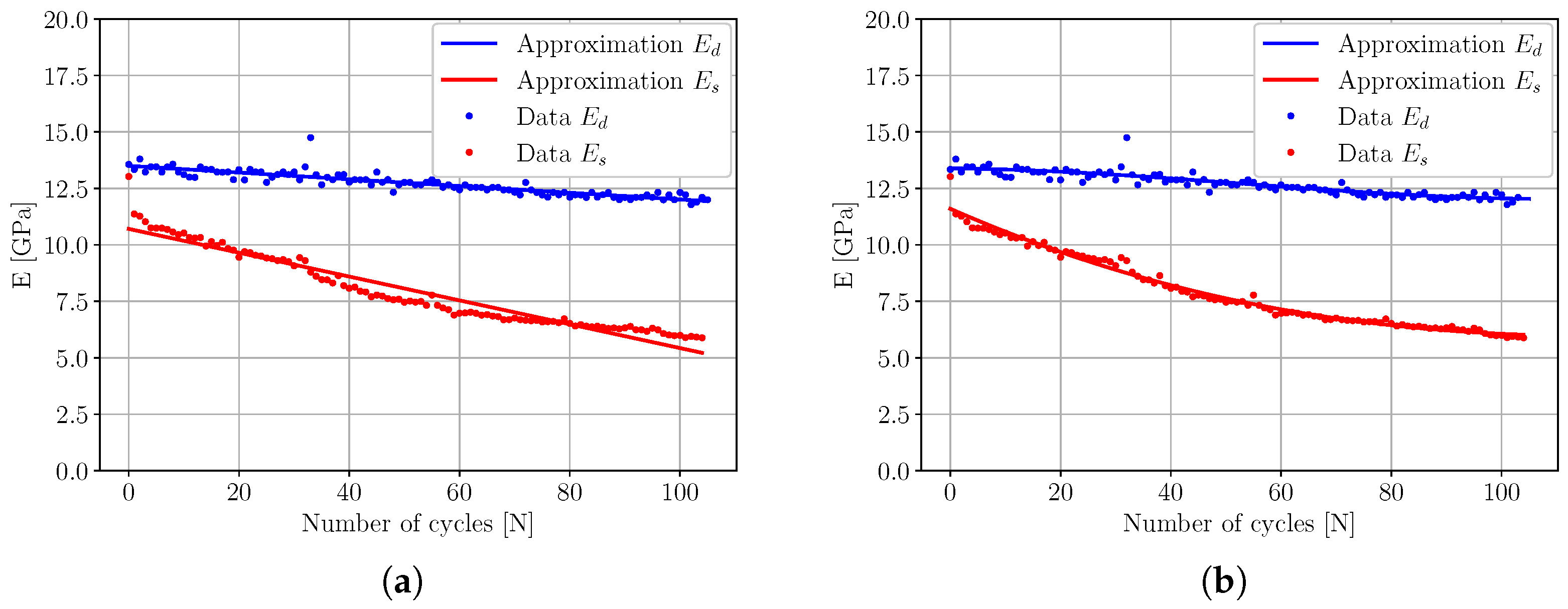
The static modulus of elasticity was calculated for each recorded load cycle. It is lower than the dynamic modulus of elasticity, which is determined from the resonance frequency, as shown in Figure 8. Both linear and cubic relationships were used to approximate the data. Given the apparent data distribution, a linear approximation was applied to the data in Figure 8a. Based on the expected behaviour—that the modulus of elasticity decreases rapidly during the initial cycles before stabilising or declining linearly—a cubic approximation was also employed, as illustrated in Figure 8b. At the end of fatigue, we anticipated a more rapid decrease in the elastic modulus. In both cases, the modulus of elasticity decreases monotonically, with the static modulus being lower than the dynamic modulus due to the viscoelastic properties of wood. These properties result in time-dependent strain effects under static loading, explaining the faster decline in the static modulus compared to the dynamic modulus [26,27]. The dynamic modulus exhibits greater scatter and is almost linear despite the cubic approximation. The relative difference between the residuals, $R_{E_d}^2$, of the linear and cubic approximations is less than 1%. The greater scatter may be due to small inconsistencies in surface condition, slight variations in moisture content, or sensor alignment during vibration measurements, all of which can affect the measurement of dynamic modulus in wood materials [26,37]. The static modulus shows less scatter and is less linear, as confirmed by the difference between the residuals $R_{E_s}^2$ in

Table 1. Coefficient of determination $R^2$ for the linear and cubic approximations of the static modulus of elasticity, $E_s$, dynamic modulus of elasticity, $E_d$, and the resonance frequency, $\omega$. The relative differences between the two approximations are also provided.

Approximation Type	${\mathit{R}}_{{\mathit{E}}_{\mathit{s}}}^2$	${\mathit{R}}_{{\mathit{E}}_{\mathit{d}}}^2$	${\mathit{R}}_{\mathit{\omega }}^2$
Linear	0.928	0.790	0.881
Cubic	0.983	0.797	0.884
Relative difference	5.61	0.89	0.35

. It is better described by a cubic approximation. The first point of the static modulus of elasticity is significantly higher than the subsequent points, which can be understood as a rapid drop in the elastic modulus at the beginning of fatigue—a phenomenon that a simple cubic approximation cannot capture. Such a phenomenon is not observed for the dynamic modulus of elasticity.

4.2. Fatigue Life Prediction

We used only linear approximations for fatigue life prediction because they are more stable when working with smaller datasets. Cubic approximations were not employed, as the difference in data deviation between linear and cubic methods is negligible, as demonstrated in Table 1. The dynamic modulus of elasticity was calculated using the resonance frequency measured between load cycles. The various approximations of the resonance frequency are shown in Figure 9. The decrease in resonance frequency from the start to the end of fatigue is approximately 35 Hz, or 6%.

We determined fatigue life using three different methods based on three variables. The variables employed in the fatigue life prediction methods were resonance frequency ($\omega$), the static modulus of elasticity ($E_s$), and the dynamic modulus of elasticity ($E_d$). In the first, simpler method, the slope of the linear approximation was used for a specific data portion. In the second simple method, the mean value of the predicted number of cycles was calculated. In the third method, we analysed the predicted number of cycles using the Weibull c.d.d. The results of all three methods, along with the corresponding errors, are presented in

Table 2. Fatigue life prediction using 40% and 100% of the data with the Weibull c.d.d. ($N_{w40}$, $N_{w100}$), the slope method, ($N_{40}$), and using an average value from all data ($N_{avg}$) for static and dynamic elastic modulus and resonance frequency ($E_s$, $E_d$, and $\omega$).

	${\mathit{\theta }}_{40}$	${\mathit{\beta }}_{40}$	${\mathit{N}}_{\mathit{w}40}$	${\mathbf{Err}}_{\mathit{w}40}$	${\mathit{N}}_{40}$	${\mathbf{Err}}_{40}$	${\mathit{\theta }}_{100}$	${\mathit{\beta }}_{100}$	${\mathit{N}}_{\mathit{w}100}$	${\mathbf{Err}}_{\mathit{w}100}$	${\mathit{N}}_{\mathbf{avg}}$	${\mathbf{Err}}_{\mathbf{avg}}$
$\omega$	101.9	3.18	90	15.1	118	11.3	110.3	4.4	105	0.94	99	6.6
$E_d$	131.5	1.98	95	10.4	147	38.7	128.3	3.03	114	7.6	115	8.5
$E_s$	68.4	2.06	48	53.9	78	26.4	89.0	2.56	73	31.1	77	27.4

. According to the first method, the best prediction, based on 40% of the data, is from $\omega$, but it is not conservative, whereas the prediction from $E_s$ is conservative, but exhibits a large relative error ($Er{r}_{40}$). The prediction with the highest relative error arises from the use of $E_d$. The second fatigue life prediction method yields the lowest relative error ($Er{r}_{avg}$) when $\omega$ is used and is also conservative. The prediction based on $E_d$ remains non-conservative, but does not have the largest relative error. The prediction based on $E_s$ has the greatest error.

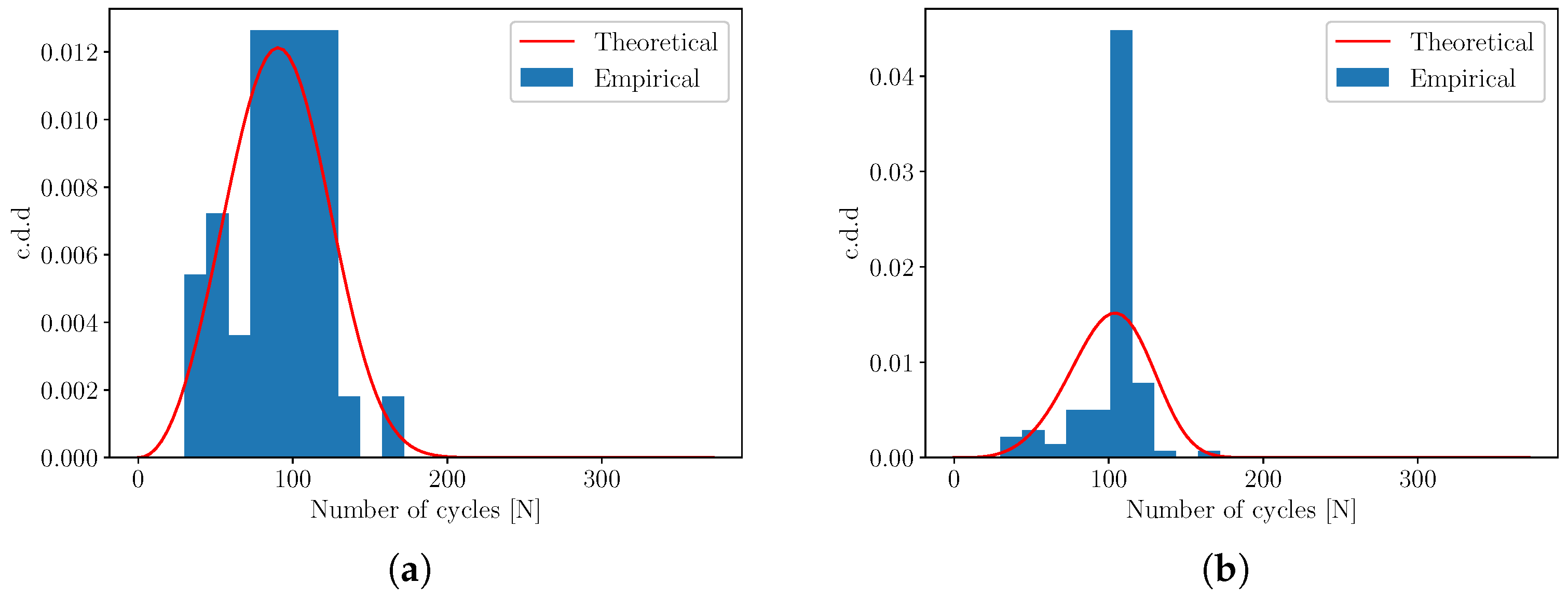
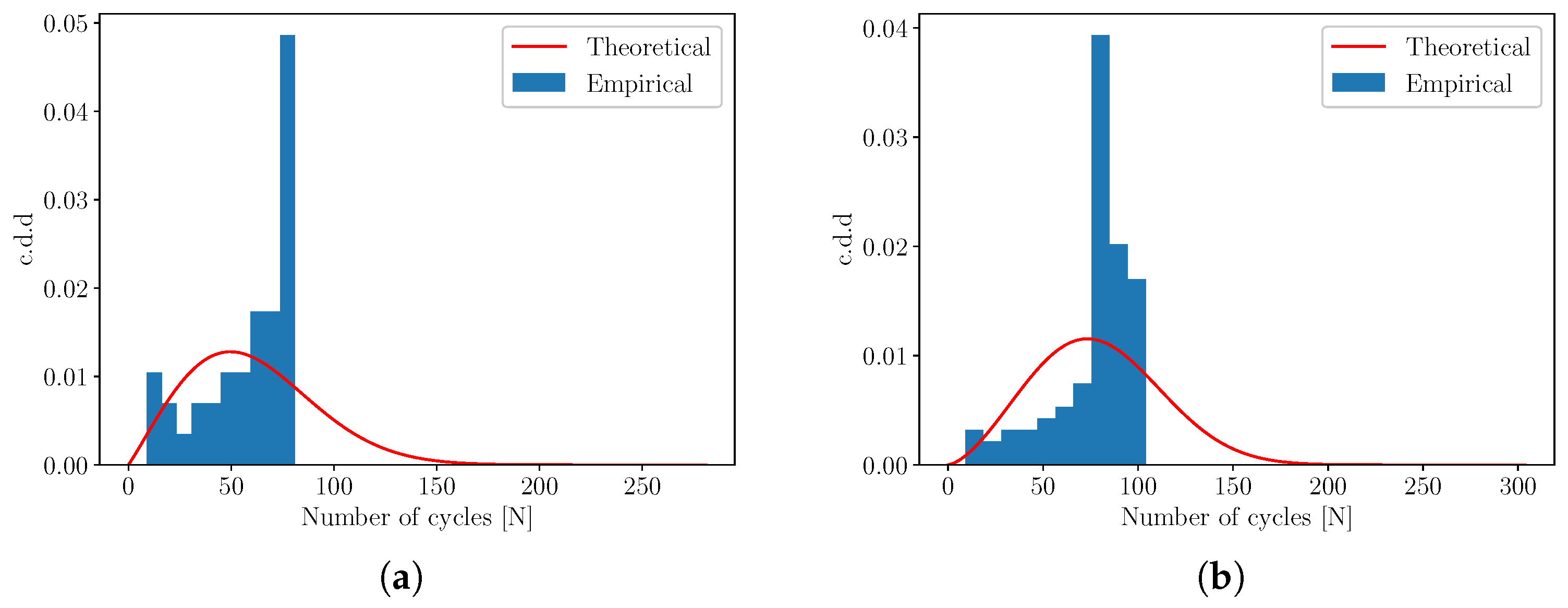
In the third and more complex method for predicting fatigue life, it was necessary to determine the number of cycles at which the theoretical distribution attains its maximum value. Table 2 presents the parameters of the Weibull c.d.d. equation—namely ${\theta }_{40}$ and ${\beta }_{40}$, for 40% of the data, and ${\theta }_{100}$ and ${\beta }_{100}$, for 100% of the data—along with the predicted number of cycles and the corresponding relative errors (${Err}_{w40}$ and ${Err}_{w100}$). The theoretical distribution of the predicted number of cycles, derived from $\omega$ at 40% and 100% of the data, resembles an approximately Gaussian curve, as illustrated in Figure 10. The prediction is conservative for both data portions and is the most accurate among all cases when using the full dataset. However, with a smaller portion of data, the prediction is less accurate than that obtained by the first method.

Figure 11 shows the distribution of the predicted number of cycles derived from $E_d$ for both data portions. For the full dataset, the distribution approximates a Gaussian curve. In contrast, the distribution for the smaller data portion is shifted to the left, indicating a lower predicted number of cycles. Owing to the near-Gaussian distribution, this prediction closely matches that obtained from the second fatigue life prediction method. The prediction is more accurate when using the full dataset, although it is less conservative than the prediction based on the smaller data portion. Furthermore the prediction from the smaller data portion is more accurate than that obtained using $\omega$.

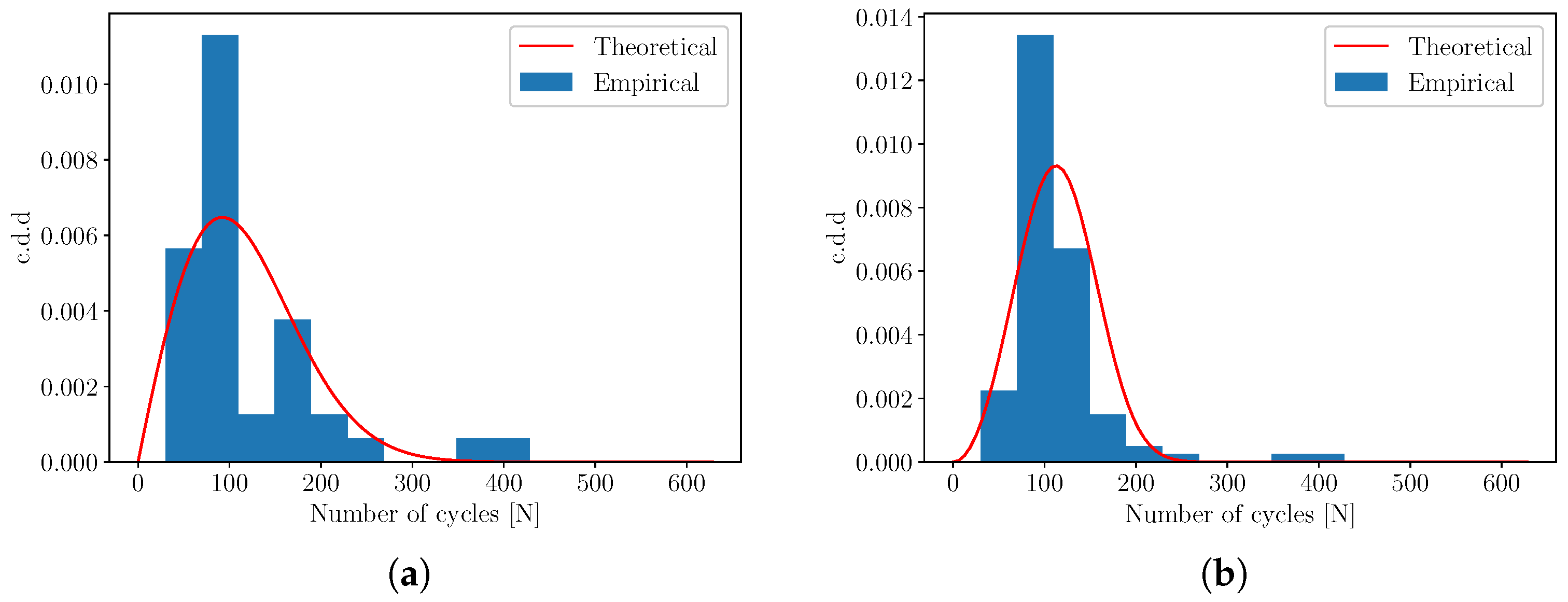
The distribution of fatigue life values predicted from a full dataset using $E_s$ resembles a Gaussian distribution (Figure 12b), but it is more skewed to the left compared to the previous two cases. This skewness increases when a smaller portion of the data is used, as shown in Figure 12a. Both predictions are conservative but exhibit substantial error. The prediction based on the smaller dataset has the largest error of all cases. Even the average of all predicted values has a smaller error than the prediction using full $E_s$ data by the third prediction method.

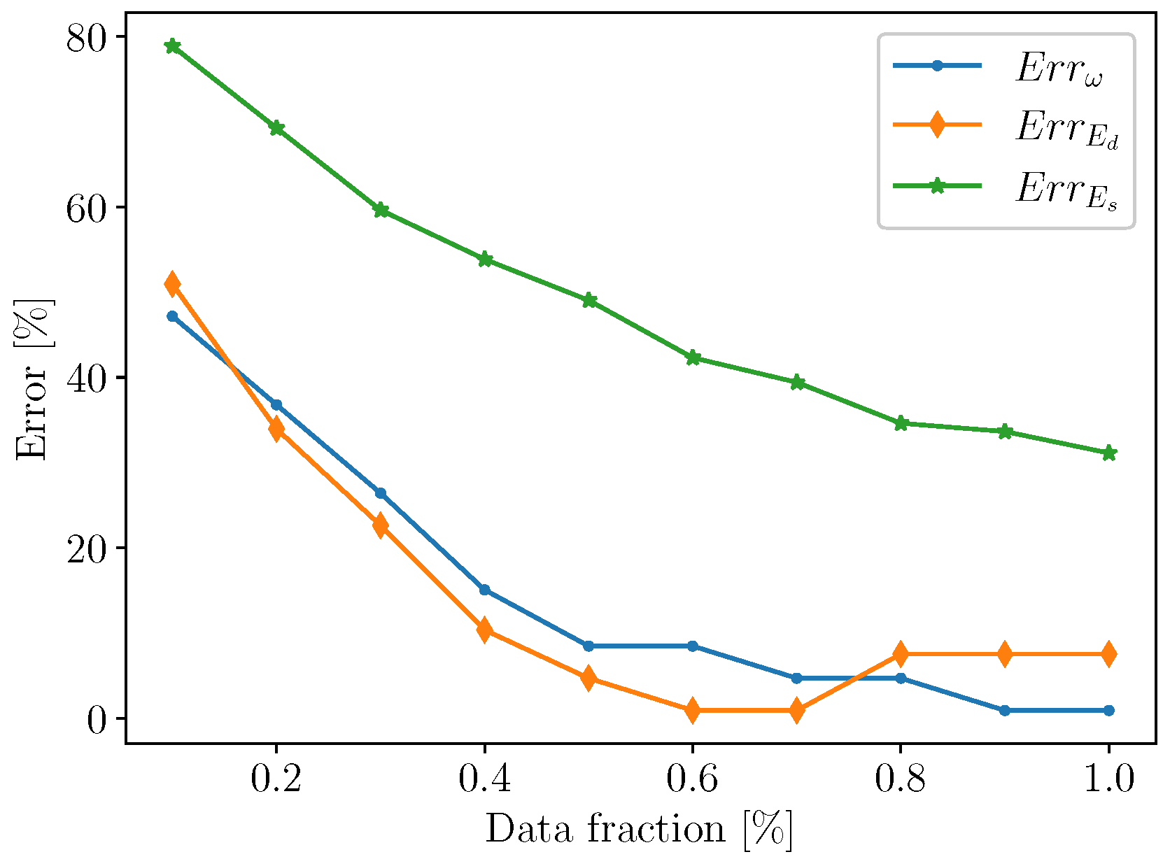
The adequacy of prediction from different data sources using the third prediction method was assessed by monitoring the relative error across various data portions employed for the prediction. Figure 13 illustrates the relative error as a function of the portion of data used for fatigue life prediction. When using $E_s$, the error is higher than in the other two cases regardless of the data portion, but it decreases monotonically, as expected. The errors associated with $E_d$ and $\omega$ exhibit a similar trend depending on the data portion. For up to 80% of the data, the error when using $\omega$ is higher than when using $E_d$. The error associated with $E_d$ increases beyond 80% of the data, with a minimum at around 70% of the data. The error as a function of the data portion when using $\omega$ remains relatively small and decreases monotonically. Although the error is not the smallest for a medium portion of the data, $\omega$ is the most suitable data type for predicting fatigue life.

4.3. Discussion

The results of this study highlight the importance of monitoring the dynamic properties of wood, such as resonance frequency, to understand the fatigue process and predict the material’s fatigue life. We found that resonance frequency is the most sensitive and reliable parameter for monitoring the fatigue of wood. The linear decrease in resonance frequency with an increasing number of cycles confirms its utility as an indicator of the material’s stiffness reduction. This trend aligns with the findings of Bedewi [23], who also observed a 25% decrease in resonance frequency in polymer composites. Similar decreases in resonance frequency have been reported for other composites [13,38]. For wood, the relative decrease in resonance frequency (6%) was lower than that observed in some other materials, indicating reduced sensitivity to cyclic loading. In spot-welded steel plates, Wang [10] also reported a decrease in resonance frequency of approximately 6%.

The difference between the static and dynamic modulus of elasticity is to be expected due to the viscoelastic properties of wood, as confirmed by Divós [27]. Under static loading, viscoelastic effects manifest as time-dependent deformations that reduce the apparent stiffness. In contrast, dynamic measurements are conducted over short periods during which these effects are minimised, resulting in higher values of the dynamic modulus. This behaviour is well documented in studies comparing static and dynamic test methods for wood [26,27]. The static modulus of elasticity decreases more rapidly as it includes deformation effects not directly captured by dynamic methods. The dynamic modulus, which is related to the resonance frequency, exhibits a more linear trend and is therefore considered one of the more accurate tools for predicting fatigue life.

The analysis using the Weibull cycle density distribution demonstrated that this method enables efficient and accurate prediction of the fatigue life of wood. The possibility of predicting fatigue life by monitoring resonance frequency during fatigue was described by Wang [10]. The Weibull distribution has also been employed to model the statistical distribution of the number of cycles, as reported by Barraza-Contreras [24]. To our knowledge, the combination of resonance frequency monitoring and the Weibull distribution has not yet been applied to fatigue life prediction of wood. Our investigations have shown that the prediction error is less than 1% when the entire dataset is utilised. Using an example, we demonstrate that the proposed method has the potential to be one of the most accurate approaches for predicting the fatigue life of wood.

One of the primary limitations of this study is the small number of test samples, which may affect the generalisability of the results. Extending the investigation to include other wood species and a larger number of specimens would allow for better validation of the proposed method, as also noted by Wang [26], who investigated the fatigue life of wood composites. It would also be beneficial to examine the effects of different types of loading and environmental factors, such as humidity and temperature, on the dynamic properties of wood. The results demonstrate significant potential for the practical application of modal analysis in monitoring the structural health of timber structures. Real-time monitoring of resonance frequency, as proposed by Omar [39], could enable early detection of damage and help prevent critical failures. However, in practice, structural timber often contains natural defects such as knots and cracks that affect its physical and mechanical properties. Further investigation of the proposed method is required to confirm its practical utility. It is important to emphasise that the proposed method has currently only been validated for homogeneous, clear spruce wood samples. Its applicability to more heterogeneous or defective wood species—where wave propagation behaviour may vary due to local density changes or structural discontinuities—remains to be explored. Therefore, the method should presently be considered case-specific rather than universal.

5. Conclusions

Research has shown that modal analysis, particularly resonance frequency monitoring, can be a reliable method for predicting the fatigue life of wood under low-cycle fatigue. Resonance frequency has been identified as the most reliable parameter, as its linear decrease accurately reflects the reduction in material stiffness. Although the static modulus of elasticity is useful, it exhibits greater variability and declines more rapidly than the dynamic modulus, limiting its reliability in fatigue life prediction. The Weibull cycle density distribution provided accurate predictions with an error of less than 1%, confirming the effectiveness of this approach.

Modal analysis holds significant potential for monitoring the mechanical condition of timber structures, as it facilitates non-destructive, real-time assessment of material integrity. A limitation of this study is the use of a single fatigue specimen, which restricts the statistical generalisability of the results. Further research should incorporate a larger number of samples, various wood species, and an examination of the effects of environmental factors. This approach offers a promising solution for enhancing the monitoring of fatigue life and the safety of timber structures.

References

1. Caicedo, D.; Lara-Valencia, L.A.; Brito, J. Frequency-Based Methods for the Detection of Damage in Structures: A Chronological Review. DYNA 2021, 88, 203–211. [Google Scholar] [CrossRef]
2. Gillich, N.; Tufisi, C.; Sacarea, C.; Rusu, C.V.; Gillich, G.R.; Praisach, Z.I.; Ardeljan, M. Beam Damage Assessment Using Natural Frequency Shift and Machine Learning. Sensors 2022, 22, 1118. [Google Scholar] [CrossRef] [PubMed]
3. Dubey, A.; Denis, V.; Serra, R. A damage identification strategy in beams based on natural frequencies shift. In Proceedings of the International Conference on Noise and Vibration Engineering (ISMA 2020), Leuven, Belgium, 7–9 September 2020. [Google Scholar]
4. Kouroussis, G.; Ben Fekih, L.; Descamps, T. Assessment of timber element mechanical properties using experimental modal analysis. Constr. Build. Mater. 2017, 134, 254–261. [Google Scholar] [CrossRef]
5. Negru, I.; Gillich, G.R.; Praisach, Z.I.; Tufoi, M.; Gillich, N. Natural frequency changes due to damage in composite beams. J. Phys. Conf. Ser. 2015, 628, 012091. [Google Scholar] [CrossRef]
6. Horta-Rangel, J.; Carmona, S.; Casta no, V.M. Shift of natural frequencies in earthquake-damaged structures: An optimization approach. Struct. Surv. 2008, 26, 400–410. [Google Scholar] [CrossRef]
7. González de Paz, L.V.G.; Ortega, N.F.; Rosales, M.B. Assessment of wood utility poles’ deterioration through natural frequency measurements. J. Civ. Struct. Health Monit. 2019, 9, 53–61. [Google Scholar] [CrossRef]
8. Shang, D. Effect of fatigue damage on the dynamic response frequency of spot-welded joints. Int. J. Fatigue 2003, 25, 311–316. [Google Scholar] [CrossRef]
9. Shang, D. Measurement of fatigue damage based on the natural frequency for spot-welded joints. Mater. Des. 2009, 30, 1008–1013. [Google Scholar] [CrossRef]
10. Wang, R.; Shang, D. Fatigue life prediction based on natural frequency changes for spot welds under random loading. Int. J. Fatigue 2009, 31, 361–366. [Google Scholar] [CrossRef]
11. Banks, H.T.; Emeric, P.R. Detection of Non-Symmetrical Damage in Smart Plate-Like Structures. J. Intell. Mater. Syst. Struct. 1998, 9, 818–828. [Google Scholar] [CrossRef]
12. Kessler, S.S.; Spearing, S.M.; Atalla, M.J.; Cesnik, C.E.S.; Soutis, C. Damage detection in composite materials using frequency response methods. Compos. Part B 2002, 33, 87–95. [Google Scholar] [CrossRef]
13. Wu, T.; Xu, C.; Li, P. A natural frequency degradation model for very high cycle fatigue of woven fiber reinforced composite. Int. J. Fatigue 2020, 134, 105398. [Google Scholar] [CrossRef]
14. Liang, Z.; Ramakrishnan, K.R.; Ng, C.T.; Zhang, Z.; Fu, J. Vibration-based prediction of residual fatigue life for composite laminates through frequency measurements. Compos. Struct. 2024, 329, 117771. [Google Scholar] [CrossRef]
15. Šraml, M.; Glodež, S.; Fajdiga, G. Fatigue Life Models of Wood: A Review. In Proceedings of the International Conference MATRIB, Vela Luka Island of Korčula, Croatia, 27–29 June 2019. [Google Scholar]
16. Klemenc, J.; Fajdiga, G. Statistical Modelling of the Fatigue Bending Strength of Norway Spruce Wood. Materials 2022, 15, 536. [Google Scholar] [CrossRef]
17. Klemenc, J.; Humar, M.; Fajdiga, G. Influence of insect damage to the fatigue life of an old larch wood. Constr. Build. Mater. 2023, 375, 130967. [Google Scholar] [CrossRef]
18. Kolesnikov, N.G.; Nazarev, D.P. Monotonic and cyclic load of pine wood under uniaxial compression: Experiments and modeling. E3S Web Conf. 2023, 458, 07021. [Google Scholar] [CrossRef]
19. Clorius, C.O.; Pedersen, M.U.; Hoffmeyer, P.; Damkilde, L. An experimentally validated fatigue model for wood subjected to tension perpendicular to the grain. Wood Sci. Technol. 2009, 43, 334–357. [Google Scholar] [CrossRef]
20. Arriaga, F.; Wang, X.; Íniguez-González, G.; Llana, D.F.; Esteban, M.; Niemz, P. Mechanical Properties of Wood: A Review. Forests 2023, 14, 1202. [Google Scholar] [CrossRef]
21. Shah, A.J.; Pandya, T.S.; Street, J. Study of variation in natural frequencies of bio-composites due to structural damage. Int. Wood Prod. J. 2020, 11, 166–172. [Google Scholar] [CrossRef]
22. Khoshmanesh, S.; Watson, S.J.; Zarouchas, D. Characterisation of fatigue damage in a thick adhesive joint based on changes in material damping. J. Phys. Conf. Ser. 2020, 1618, 022058. [Google Scholar] [CrossRef]
23. Bedewi, N.E.; Kung, D.N. Effect of fatigue loading on the modal properties of composite structures and its utilization for prediction of residual life. Compos. Struct. 1997, 37, 357–371. [Google Scholar] [CrossRef]
24. Barraza-Contreras, J.M.; Pi na-Monarrez, M.R.; Molina, A. Fatigue-Life Prediction of Mechanical Element by Using the Weibull Distribution. Appl. Sci. 2020, 10, 6384. [Google Scholar] [CrossRef]
25. Ibrahim, S.R. Random Decrement Technique for Modal Identification of Structures. J. Spacecr. Rockets 1977, 14, 696–700. [Google Scholar] [CrossRef]
26. Wang, Z.; Li, L.; Gong, M. Measurement of dynamic modulus of elasticity and damping ratio of wood-based composites using the cantilever beam vibration technique. Constr. Build. Mater. 2012, 28, 831–834. [Google Scholar] [CrossRef]
27. Divós, F.; Tanaka, T. Relation Between Static and Dynamic Modulus of Elasticity of Wood. Acta Silv. Lignaria Hung. 2005, 1, 105–110. [Google Scholar] [CrossRef]
28. ASTM E606/E606M-12; Standard Test Method for Strain-Controlled Fatigue Testing. ASTM Standards: West Conshohocken, PA, USA, 2012.
29. Thomson, W.T. Theory of Vibration with Application, 4th ed.; Taylor and Francis: New York, NY, USA, 2003; pp. 268–289. [Google Scholar]
30. Tongue, B.H. Principles of Vibration, 2nd ed.; Oxford University Press: New York, NY, USA, 2001. [Google Scholar]
31. Merhar, M. Determination of Dynamic and Static Modulus of Elasticity of Beech Plywood. Les/Wood 2020, 69, 59–69. [Google Scholar] [CrossRef]
32. Straže, A.; Fajdiga, G.; Gospodarič, B. Nondestructive characterization of dry heat-treated fir (Abies alba Mill.) timber in view of possible structural use. Forests 2018, 9, 776. [Google Scholar] [CrossRef]
33. Weibull, W. A Statistical Theory of The Strength of Materials; Generalstabens Litografiska Anstalts Förlag: Stockholm, Sweden, 1939; Volume 151, pp. 1–45. [Google Scholar]
34. Benard, A.; Bos-Levenbach, E.C. The Plotting of Observations on Probability; van Dantzig, D., Hemelrijk, J., Eds.; Mathematisch Centrum: Amsterdam, The Netherlands, 1955. [Google Scholar]
35. ISO 3129:2019(en); Wood—Sampling Methods and General Requirements for Physical and Mechanical Testing of Small Clear Wood Specimens. ISO Standards: Geneva, Switzerland, 2019.
36. Ogawa, K.; Shimizu, K.; Yamasaki, M.; Sasaki, Y. Fatigue behavior of Japanese cypress (Chamaecyparis obtusa) under repeated compression loading tests perpendicular to the grain. Holzforschung 2017, 71, 499–504. [Google Scholar] [CrossRef]
37. Kliger, R.; Olsson, A.; Perstorper, M. Measurement of dynamic modulus of elasticity in timber structures using frequency analysis of flexural vibrations. Wood Sci. Technol. 1997, 31, 431–441. [Google Scholar]
38. Abo-Elkhier, M.; Hamada, A.A.; Bahei El-Deen, A. Prediction of Fatigue Life of Glass Fiber Reinforced Polyester Composites Using Modal Testing. Int. J. Fatigue 2014, 69, 28–35. [Google Scholar] [CrossRef]
39. Omar, I.; Khan, M.; Starr, A. Suitability Analysis of Machine Learning Algorithms for Crack Growth Prediction Based on Dynamic Response Data. Sensors 2023, 23, 1074. [Google Scholar] [CrossRef] [PubMed]
Figure 1. Deflection of the beam in the first vibration mode. The solid line represents the beam on supports (red dots), while the dashed line represents the beam after excitation.
Forests 16 01324 g001
Figure 2. Theoretical model of a symmetrical three-point load for calculating deflection.
Forests 16 01324 g002
Figure 3. Test setup for static fatigue bending tests and vibration resonance analysis: specimen, microphone, analogue-to-digital converter (ADC), microcontroller ( μ C), personal computer (PC), hammer, electromagnet (EM), and electromagnet driver.
Forests 16 01324 g003
Figure 4. Experiment setup.
Forests 16 01324 g004
Figure 5. Specimen state during fatigue loading. (a) First visible crack during the 105th load cycle; (b) damaged state during the final load cycle.
Forests 16 01324 g005
Figure 6. Fracture surface. (a) Static test; (b) fatigue test.
Forests 16 01324 g006
Figure 7. Selection of two points on the loading segment of the force–displacement curve to determine the static modulus of elasticity.
Forests 16 01324 g007
Figure 8. Approximation of static and dynamic moduli of elasticity: (a) linear approximation; (b) cubic approximation.
Forests 16 01324 g008
Figure 9. Approximation of resonance frequency. (a) Linear approximation; (b) cubic approximation.
Forests 16 01324 g009
Figure 10. Weibull c.d.d of the predicted number of cycles based on resonance frequency data. (a) A total of 40% of the data; (b) full dataset.
Forests 16 01324 g010
Figure 11. Weibull c.d.d of the predicted number of cycles based on dynamic elastic modulus data. (a) A total of 40% of the data; (b) full dataset.
Forests 16 01324 g011
Figure 12. Weibull c.d.d of the predicted number of cycles based on static elastic modulus data. (a) A total of 40% of the data; (b) full dataset.
Forests 16 01324 g012
Figure 13. Relative error in correlation with data fraction used for fatigue life prediction using Weibull c.d.d.
Forests 16 01324 g013