Article

Carbon Emission Prediction Following Pinus koraiensis Plantation Surface Fuel Combustion Based on Carbon Consumption Analysis

Key Laboratory of Sustainable Forest Ecosystem Management-Ministry of Education, College of Forestry, Northeast Forestry University, Harbin 150040, China
*
Author to whom correspondence should be addressed.
These authors contributed equally to this work.
Forests 2025, 16(5), 726; https://doi.org/10.3390/f16050726
Submission received: 12 March 2025 / Revised: 10 April 2025 / Accepted: 22 April 2025 / Published: 24 April 2025
(This article belongs to the Special Issue Fire Ecology and Management in Forest—2nd Edition)

Abstract

:
The accurate measurement of surface fire carbon emissions is critical for assessing their impact on carbon sinks and role in climate change. This study aims to investigate the relationships between surface fire behaviour characteristics and carbon consumption for Pinus koraiensis plantation forests and construct a carbon consumption prediction model. A total of 288 combustion experiments were conducted on a laboratory burning bed using varying fuel loads, moisture contents, and slope conditions, with measurements taken of surface fire behaviour characteristics and the carbon content of combustion ash. The Byram fireline intensity model was reintegrated to build a predictive model for fuel combustion carbon consumption, and the model parameters were adjusted based on the results of the combustion experiments. The direct use of the Byram fireline intensity model parameters predicted surface fire carbon consumption in Pinus koraiensis plantation forests with significant errors (R2 = 0.75; MAE = 0.197 kg m−2; MRE = 66.76%). After the parameters were modified using the combustion experiment data, the new model yielded R2 = 0.75, MAE = 0.087 kg m−2, and MRE = 28.28%. This study significantly improved the accuracy of the new model in predicting the carbon consumption of surface fuel combustion in Pinus koraiensis plantation forests.

1. Introduction

Forests are the most significant carbon reservoir on land and function as long-term carbon stores, playing unique and vital roles in the global carbon cycle and climate change [1,2,3]. Forest vegetation stores 359–373 Pg of carbon [4]. Terrestrial ecosystems, of which forests are the primary contributors, remove approximately 3 Pg of carbon annually, or 30% of all CO2 resulting from the combustion of fossil fuels and net deforestation [5]. However, various disturbances have the potential to dislocate the carbon stored in forests [6]. One of the most significant disruptions to forests is fire, which makes it more difficult for them to develop sustainably and reduces their capacity as self-healing forest ecosystems [7]. Globally, 300–460 million hectares of forests are disturbed by fires each year (approximately 4% of Earth’s vegetation area) [8,9], and carbon emissions due to fires equal approximately 2.2 Pg [10], or one-third of the total carbon emissions from fossil fuel combustion at present; moreover, a large amount of carbon is emitted into the atmosphere during fires, reducing the potential capacity of forests to absorb carbon [11,12]. In recent decades, forest fires have lengthened in cycle and intensified in both frequency and magnitude due to climate and land cover changes, leading to a gradual increase in carbon emissions [13,14,15,16]. New evidence suggests forest fires’ release of large amounts of greenhouse gases, such as CO2, into the atmosphere exacerbates climate change in a positive feedback manner [17,18,19]. Therefore, the accurate estimation of carbon emissions from forest fires is essential for understanding the impacts of forest fires on carbon sinks and assessing the potential capacity of forest fires to contribute to climate change [20,21].
The current prediction of carbon emissions from forest fires mainly uses the models proposed by Seiler and Crutzen [22] and Ward and Hao [23]. A top-down approach is used, with C = a × B × CC × fc, where C represents the combustion emissions, a represents the area burned, B represents the fuel load, and CC and fc represent the combustion efficiency and fuel carbon content (also known as the conversion factor), respectively. The model supports strategies to mitigate the risk of forest fires and climate change. With the development of computers, satellites, remote sensing, and other technologies, geographic information and spatial data have been widely used for predicting carbon emissions from forest fires on large scales. Satellites have been used to gather data on burned areas and fuel consumption. A biogeochemical fuel model estimating fuel loads of 0.5 has been used to calculate carbon emissions from forest fires using the fuel’s carbon content [24,25]. However, remote sensing resolution, spatial scale, fuel type, and other factors lead to highly inaccurate predictions of carbon emissions [26]. Surface fires are fires that extend and spread along the forest floor surface, accounting for more than 90% of the total number of forest fires [27], and are the primary stage and an essential component of forest fires, emitting more than half of the carbon released by forest fires. The United States FOFEM and Consume first-order fire effects models assume the complete combustion of surface fuels (i.e., 100% combustion efficiency), which is unreasonable [28,29] and overestimates the carbon emissions from forest fires, with an error of up to 30% or more [30]. Benali et al. [31] reported that small changes in the fuel mix could lead to significant changes in fire behaviour and that using fixed coefficients to estimate carbon emissions from forest fires is inconsistent with the characteristics of actual forest fires. Thus, it is necessary to incorporate varying degrees of fire severity into estimating carbon emissions. In addition, meteorological factors such as wind and topographical factors such as slope have well-known effects on fire behaviour, which can also lead to differences in surface fire carbon emissions. In summary, there is an inextricable relationship between surface fire behaviour and carbon emissions. Hence, researching forest fire behaviour characteristics and forest fire carbon emissions to provide scientific and technological guidance for forest fire management is essential in the current research on fire carbon emissions.
Planted forests are an integral part of the forest ecosystem, and the current area of planted forest in China is 220 million ha, accounting for 5% of the world’s forest area and ranking first in the world [32]. Recently, the forest areas in the southwest and northeast regions of China have increased by 40,000–440,000 ha per year via planted forests and have become essential parts of China’s forest ecosystem [33]. Heilongjiang Province is a large province of forest resources in China and also a region with a high incidence of forest fires. Plantation forests are mostly coniferous pure forests with simple stand structures, high forest oil and grease contents, and weak abilities to withstand forest fires and other disasters [34], whereas carbon emissions from plantation forests gradually increase with increasing forest age [35]. Pinus koraiensis plantations constitute one of the main silvicultural species in the region; these plantations are rich in large amounts of oil and grease, and the surface fuels are mostly homogeneous beds, which present a significant risk of forest fires [36]. This study used the surface fuels of Pinus koraiensis plantation forests in Northeast China as experimental materials. We conducted laboratory combustion experiments using different combinations of slopes, fuel loads, and fuel moisture contents to analyse the relationships between the characteristics of forest fire behaviour and fuel carbon consumption and to establish a model for the carbon consumption of surface fuel combustion in Pinus koraiensis plantation forests. The results of this study can provide essential data for fire researchers, provide a research basis for subsequent research in forest fire science, and be of practical significance for constructing a fuel-burning carbon consumption prediction system applicable to China.

2. Materials and Methods

The experimental materials in this study were surface fuels from Pinus koraiensis plantations forests. The samples were obtained from the Experimental Forestry Farm of Northeast Forestry University in Maoershan (45°14′–45°29′ N, 127°29′–127°44′ E), where all the field data were collected. The forest is located in Shangzhi City, Heilongjiang Province, and has a temperate monsoon climate. The average annual temperature is 2.8 °C, and the annual precipitation is 723.8 mm. The forest area belongs to the western slope of Zhangguangcailing of the Changbai Mountain System and features low hills and gentle slopes; most of the slopes range from 10° to 35°, with an average altitude of 300 m. The forest coverage is 85%, and the main species of trees are Pinus koraiensis, Quercus mongolica, and Betula platyphylla.
The Pinus koraiensis plantations’ forest surface fuels were collected in August 2022. Before the samples were collected, we set up five 30 m × 30 m standard sample plots within the forest and conducted a per-wood check of each tree within the plots to determine the stand characteristics. Five 1 m × 1 m sample plots (four in the corners and one in the centre) were set up within each sample plot to collect all surface dead leaves within the sample plots by destructive sampling, which was used to measure the surface fuel load (see Table 1 for the preliminary information on the sample plots). After the measurements, we collected dead leaves from the sample site and transported them back to the laboratory to be ventilated and preserved for the combustion experiments. We randomly selected intact dead leaves from Pinus koraiensis plantations from the samples. The calorific value of the dead leaves on the surface of the Pinus koraiensis plantations was 22,478 KJ kg−1, the surface area-to-volume ratio was 6864.3 m−1, and the particle density was 396.4 kg m−3.

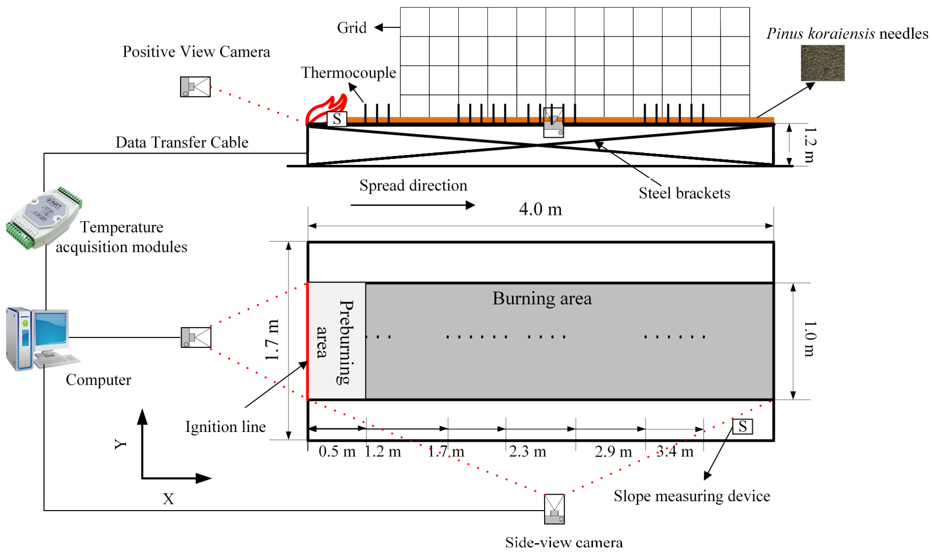
2.1. Combustion Experiment

The burning bed is in the Forest Fire Behavior Laboratory at Northeast Forestry University. It is 20 m long, 10 m wide, and 8 m high, with a passive exhaust device on the roof. The laboratory is semi-open to provide a basis for conducting indoor simulations of natural environments in the field. The combustion experiments were conducted on a tiltable burning bed that was 4 m long (X direction) by 1.7 m wide (Y direction). The tilt angle was adjustable from 0° to 40°. The area used for combustion was 4 m long and 1.3 m wide (Figure 1). The combustion experiments took place from September to October 2022 during the autumn fire season in Northeast China. The meteorological conditions (temperature and humidity) in the laboratory and during the fire season were approximately the same, making the combustion experiment closer to the actual fires in the field and meeting the needs of scientific research on forest fires.

2.1.1. Fuel Pretreatment

Based on the data from the sample plots investigated in the field, we set the fuel loads to 0.4, 0.8, 1.2, and 1.6 kg m−2 to be closer to the actual surface fire behaviour and carbon consumption characteristics in the field (Table 1).
During the precombustion experiments, we found that extinction occurred when the fuel moisture content exceeded 20%. As this study predicts carbon consumption based on fire behaviour characteristics under open-flame combustion, we set the fuel moisture content to 5%, 10%, and 15%, i.e., at three levels, to ensure that the fuel was in an open-flame combustion state and that the experiments would be reproducible. The fuel moisture content (FMC) can be calculated using Equation (1):
FMC = W H W D W D × 100 %
where FMC is the fuel moisture content (%), WH is the fuel wet weight (kg m−2), and WD is the fuel dry weight (kg m−2).
Geng et al. [37] explained the process of preparing fuel moisture content. We used the actual fuel moisture content in the model development to make the subsequent model development and statistical analysis more reasonable. For ease of description, we used the preset fuel moisture content when analysing the data and plotting the graphs.
The study area selected for this study was primarily a gently sloping terrain of low hills, with slopes generally not exceeding 35° [38]. To be as close as possible to the real slope in the field when performing the slope setting, we set the slope to 0°, 5°, 10°, 15°, 20°, 25°, 30° and 35° for a total of 8 levels.

2.1.2. Laboratory Combustion Experiments

We set the fuel bed area to 4 m × 1 m. Before the experiments started, the configured fuel was distributed as uniformly as possible on the burning bed according to the fuel load, fuel moisture content, and slope configuration of the experimental setup. Before the start of each experiment, indicators such as air temperature, air humidity, relative humidity, fuel wet weight, and bed depth were measured. Air humidity and relative humidity were measured using a hand-held weather station (Kestrel 4500, Nielsen-Kellerma, Boothwyn, PA, USA), and fuel wet weight was measured using a balance with an accuracy of 0.1 g. Fuel bed depth was measured at four random locations per square metre of the fuel bed. Before each experiment, 15 mL of alcohol was sprayed evenly across the entire width of the fuel bed to ignite the fuel. The study included 96 combinations of fuel loadings, fuel moisture contents, and slopes. We performed three repetitions of each combination for 288 combustion experiments to reduce errors. To prevent the residual heat from the previous combustion experiment from affecting the next one, we used an infrared camera to measure the temperature of the burning bed to ensure that it had cooled to ambient temperature.
In this study, we employed the thermocouple method to determine the rate of spread (ROS) of surface fuel in Pinus koraiensis plantations [39]. This was accomplished by deploying one thermocouple every 0.1–0.5 m from the ignition end of the fuel bed for a total of 20 thermocouples. The moment when the thermocouple temperature first rose to 254 °C (i.e., the Pinus koraiensis plantation ignition point) was extracted as when the fire front reached that thermocouple. The time was fitted based on when the thermocouple reached the ignition temperature, and the slope of this fit was the ROS for this combustion experiment [40].
The flame length was defined as the distance from the centre point of the bottom to the top of the flame. In this study, we measured the flame length at four positions in the fuel bed using the grid method [41]. Once the fire was completely extinguished, all remaining ash was collected, weighed, and stored in sealed bags. Fuel consumption was calculated as the difference between the initial fuel dry weight and the ash weight remaining after combustion. The fireline intensity was determined using the Byram [42] model Equation (2):
I = h W R
where I is the fireline intensity (kW m−1), h is the fuel low calorific value (KJ kg−1), W is the fuel consumption (kg m−2), and R is the rate of spread (m s−1).

2.1.3. Fuel Carbon Consumption Measurement

When the ashes remaining after combustion were collected, the fuel was not burned completely or not burned at all. Therefore, before the carbon content of the samples was measured, all the combustion residues from each experiment were pulverised in a grinder through an 80 mesh sieve and baked at 60 °C until a constant weight was reached. We determined the carbon content of the samples using an HT1300 Total Carbon Analyser (Analytik Jena AG, Jena, Germany). We randomly selected six samples from the surface fuels collected from the Pinus koraiensis plantation forest as the initial carbon content, and the measured value was 48.30%. The fuel combustion carbon consumption is calculated as shown in Equation (3):
W C = W B W 0 W J W S
where WC is the fuel carbon consumption (kg m−2), WB is the initial fuel carbon content (a dimensionless fraction of a unit, 0 < WB < 1), W0 is the initial fuel dry weight (kg m−2), WJ is the ash weight remaining after combustion (kg m−2), and WS is the combustion ash carbon content (a dimensionless fraction of a unit, 0 < WS < 1).

2.2. Modelling Fuel Carbon Consumption

2.2.1. Modelling of Fuel Consumption and Carbon Consumption

Fuels are affected by the fuel load, fuel moisture content, and slope during combustion, resulting in differences in fuel consumption. This study used a single fuel with the same initial carbon content. We first plotted and fitted a scatter plot of fuel consumption versus fuel carbon emissions to obtain a fitted equation to explore the relationship between fuel consumption and carbon consumption (Equation (4)).
W C = c W
where c is the dimensionless coefficient of fit (0 < c < 1) between fuel consumption and carbon consumption.

2.2.2. Fuel Carbon Consumption Model

In this section, the model for predicting fuel carbon consumption was constructed by reorganising Byram’s fireline intensity equation and incorporating the coefficient c from Equation (4) into the equation. Byram [42] proposed two equations to calculate the fireline intensity. The first calculates the fireline intensity in terms of the fuel low heating value, fuel consumption, and ROS, as shown by Equation (2). The second method calculates the fireline intensity using the exponential equation for flame length [42]. We equated Byram’s two equations for calculating fireline intensity, thereby deriving Equation (5):
h W R = a L f b
where Lf is the flame length (m), and a and b are empirical coefficients. In the Byram fireline intensity model, a = 258 and b = 2.17. By substituting Equation (5) into Equation (4), we derived Equation (6), which serves as the predictive model for fuel carbon consumption.
W C = c a L f b h R

2.3. Data Processing and Analysis

We used Microsoft Office 2021 (Microsoft Corporation, Redmond, WA, USA) and IBM Statistical Package for the Social Sciences (SPSS) 27 (IBM Corporation, Armonk, NY, USA) for preliminary statistics and plotted the data on the environment, fire behaviour characteristics, and carbon consumption obtained and calculated in the combustion experiments. Histograms were plotted using Origin 2021 (OriginLab Corporation, Northampton, MA, USA) to analyse the fire behaviour characteristics with varying fuel loads, moisture contents, and slope conditions. The values of a and b in Equation (6) were recalculated in MATLAB 2018b (MathWorks, Natick, MA, USA) using the least squares method and were combined with the fire behaviour characteristic data obtained from the combustion experiments, and the prediction effect of the newly constructed fuel carbon consumption model was evaluated using the mean absolute error (MAE), the mean relative error (MRE), the mean bias error (MBE), and the R-square (R2).

3. Results and Analysis

3.1. Data Statistics of Combustion Experiment

Table 2 shows the preliminary statistical results of the variables and data from the combustion experiments, including the average, extreme, and percentile values. It can be seen that the fuel moisture content utilised for the experiments is relatively accurate; thus, it can be used for statistical analysis and model construction of experimental results. All the combustion experiments involved low-intensity combustion concerning the range of variation in the ROS and fireline intensity.

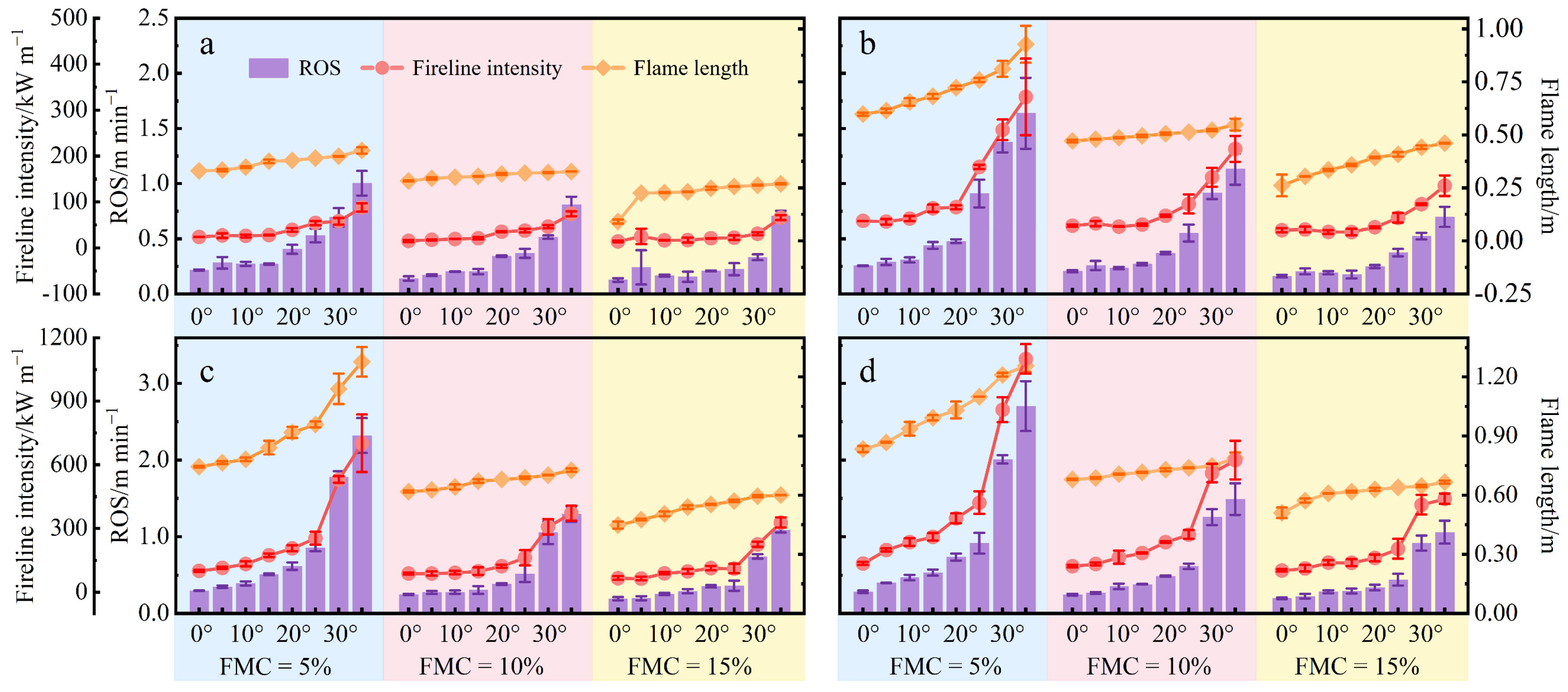
3.2. Fire Behaviour Characteristics

3.2.1. Observed ROS

The ROS is an essential indicator of fire behaviour characteristics, and its speed directly reflects the difficulty of fire suppression. In this study, we investigated the surface fuel ROS of Pinus koraiensis plantation forests for different fuel loads, fuel moisture contents, and slope conditions, and their change characteristics are shown in Figure 2. The ROS increases as the fuel load increases. This increase is because the increase in fuel load increases the mass of fuel directly involved in combustion, which releases more heat and causes more heat to be absorbed by the unburned fuel in front of it, thus increasing the ROS. The ROS decreases as the fuel moisture content increases. When the fuel is ignited, the water is first heated to its boiling point and completely vaporised before the fuel ignites. After the fuel ignites, the adjacent water in the fuel gradually evaporates as the fire spreads. Therefore, as the fuel moisture content increases, the latent heat of vaporisation required by the moisture increases, increasing the amount of energy required to ignite the fuel and thus decreasing the ROS. Moreover, the moisture in the fuel is released into the air as water vapour, resulting in a lower concentration of oxygen involved in combustion and, thus, a lower ROS. The ROS generally tends to increase as the slope increases. As the slope increases, the flame moves closer to the unburned fuel in front of it, causing the unburned fuel to absorb more heat and thus reach its ignition point faster, which manifests as an increase in the ROS. The trend of the ROS with slope shows that the ROS increases more slowly when the slope is 25° or less, whereas the ROS increases significantly when the slope exceeds 25°. These results suggest that the ROS is not simply linearly related to slope but may be a piecewise-continuous function. The reason for this may be that, as the slope increases, the flame gradually approaches the unburned fuel in front of it, and when the slope exceeds a certain threshold, the heat transfer mode of the flame changes from radiation-based heat transfer to convection-based heat transfer. In this study, the shift in the heat transfer mode occurred at approximately 25°. This study revealed that the ROS decreased with the increase in slope under certain slope conditions. For example, with the fuel load = 0.4 kg m−2, FMC = 15%, and slope = 5°, the ROS = 0.240 m min−1. However, with the fuel load = 0.4 kg m−2, FMC = 15%, and slope = 10°, the ROS = 0.166 m min−1. The reason for this difference may be that, under certain combinations of fuel load and fuel moisture content, there is a threshold between the ROS and slope below or above which the ROS decreases.

3.2.2. Flame Length

Flame length is one of the most intuitive phenomena of forest burning. It can be estimated directly at the fire scene by visual inspection and, to some extent, by the direct estimation of fireline intensity. Figure 2 shows that the flame length increases with the increase in fuel load within the gradient range of the experimental setup. This occurs because, as the fuel load increases, more effective fuel is involved in combustion, and more heat is released, increasing the flame length. The flame length becomes shorter as the fuel moisture content increases. As the fuel moisture content increases, the energy required for the latent heat of vaporisation of water increases, and the proportion of heat released from fuel combustion used for the latent heat of water vaporisation increases, thus decreasing the flame length. The flame length increases with the increase in slope. This is because, under the effect of slope, the flame is tilted toward the unburned fuel in the front, and the distance between the flame and this unburned fuel is shortened so that this unburned fuel reaches its ignition point more quickly and burns, thus increasing the flame length.

3.2.3. Fuel Consumption

Fuel consumption is one indicator used to quantify the heat released from fuel combustion and the extent of fire damage. Figure 3 shows the variation in fuel consumption with the influencing factors of the experimental setup. The effect of the fuel moisture content on fuel consumption was not significant. This may be because sufficient oxygen is obtained with a low fuel moisture content during fuel combustion, resulting in more complete combustion. However, as the fuel moisture content increases, water evaporation decreases the oxygen concentration, whereas the heat required to ignite the fuel increases, and the residence time of the flame after ignition increases, resulting in a longer fuel combustion time. Therefore, in this study, the change in the amount of fuel consumed due to the increase in fuel moisture content was insignificant. Fuel consumption generally tends to decrease slowly with the increase in slope. This is because, as the slope increases, the ROS increases, and the flame length becomes longer, resulting in a shorter flame residence time. This leads to insufficient fuel combustion, which manifests as a decrease in fuel consumption. However, combustible consumption tends to increase under some conditions rather than decrease as the slope increases. This may be because this study collected and weighed the combustion residual ash after the fire was entirely extinguished (i.e., once it became completely smokeless). The incompletely burned fuel continued to smoulder negatively as the flame passed through it; therefore, in some cases, the fuel consumption increased as the slope increased.

3.2.4. Fireline Intensity

Fireline intensity is an essential indicator for assessing the intensity of forest fires. As shown in Figure 2, the fireline intensity increases as the increase in fuel load increases. An increase in fuel load directly increases the mass of fuel involved in combustion, which increases the heat released from the fuel, leading to increases in the ROS and flame length. The fireline intensity is calculated directly from the product of the ROS and the fuel consumption and, therefore, shows an increase in the fireline intensity with the increase in fuel load. The fireline intensity decreases with the increase in fuel moisture content because the fuel moisture content has a significant inhibitory effect on combustion, resulting in a lower ROS. Additionally, in this study, the fuel moisture content has no significant effect on fuel consumption; therefore, the fireline intensity decreases with the increase in fuel moisture content and increases with the increase in slope. Based on Figure 2 and Figure 3, the increasing trend of fireline intensity is consistent with the ROS and generally opposite to that of fuel consumption. This may be because the increase in the ROS with slope is more significant than the decrease in fuel consumption, thus leading to an increase in the intensity of the fireline with slope.

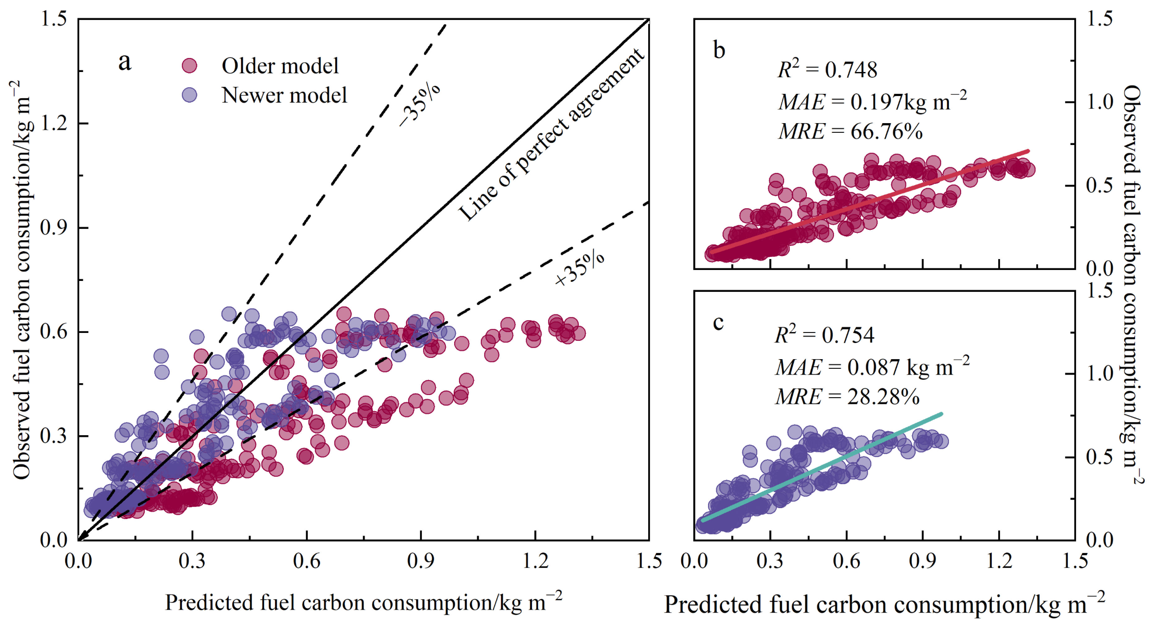
3.3. Modelling of Fuel Carbon Consumption

3.3.1. Relationship Between Fuel Consumption and Carbon Consumption

Figure 3e shows that fuel consumption has a highly significant linear relationship with carbon consumption, R2 = 0.99 (confidence interval of 95%). This indicates that the variation in fuel carbon consumption with different fuel loads, fuel moisture contents, and slopes is the same as that in fuel consumption. Therefore, the variation in fuel carbon consumption is not being analysed in terms of characterisation. The slope of the fitted line in Figure 3e is the value of the coefficient c in Equation (4).
We substituted c = 0.46 into Equation (6) and further fitted the values of a and b in Equation (6) using the measured values of surface fuel ROS, flame length, and fuel carbon consumption in Pinus koraiensis plantation forests, obtaining a = 418.18 and b = 2.55. Substituting the values of a and b into Equation (6) yields a model of carbon consumption from surface fuel combustion in Pinus koraiensis plantation forests (Equation (7)):
W C = 192.64 L f 2.55 h R
Figure 4 shows a scatter plot of the model predictions versus the observed fuel carbon consumption. Figure 4a shows that the old-model-predicted fuel combustion carbon consumption had a significant error and was often overpredicted. After the parameters are modified, the new model shows a significant improvement over the old model, with most predictions lying within ± 35%, and the results are closer to the perfect line of agreement. However, a large dispersion can still be observed.
Figure 4b,c shows the scatter plots of the predicted and observed values. The old-model-predicted values of R2 = 0.75; MAE = 0.197 kg m−2; and MRE = 66.76%; the new-model-predicted values of R2 = 0.75; MAE = 0.087 kg m−2; and MRE = 28.28%. Compared with the old model, the new model predicted a 0.006 increase in R2 and 0.110 kg m−2 and 38.48% decreases in MAE and MRE, respectively, for fuel combustion carbon consumption. Overall, the prediction accuracy of the new model in predicting the carbon consumption of surface fuel combustion in Pinus koraiensis plantation forests was significantly improved.

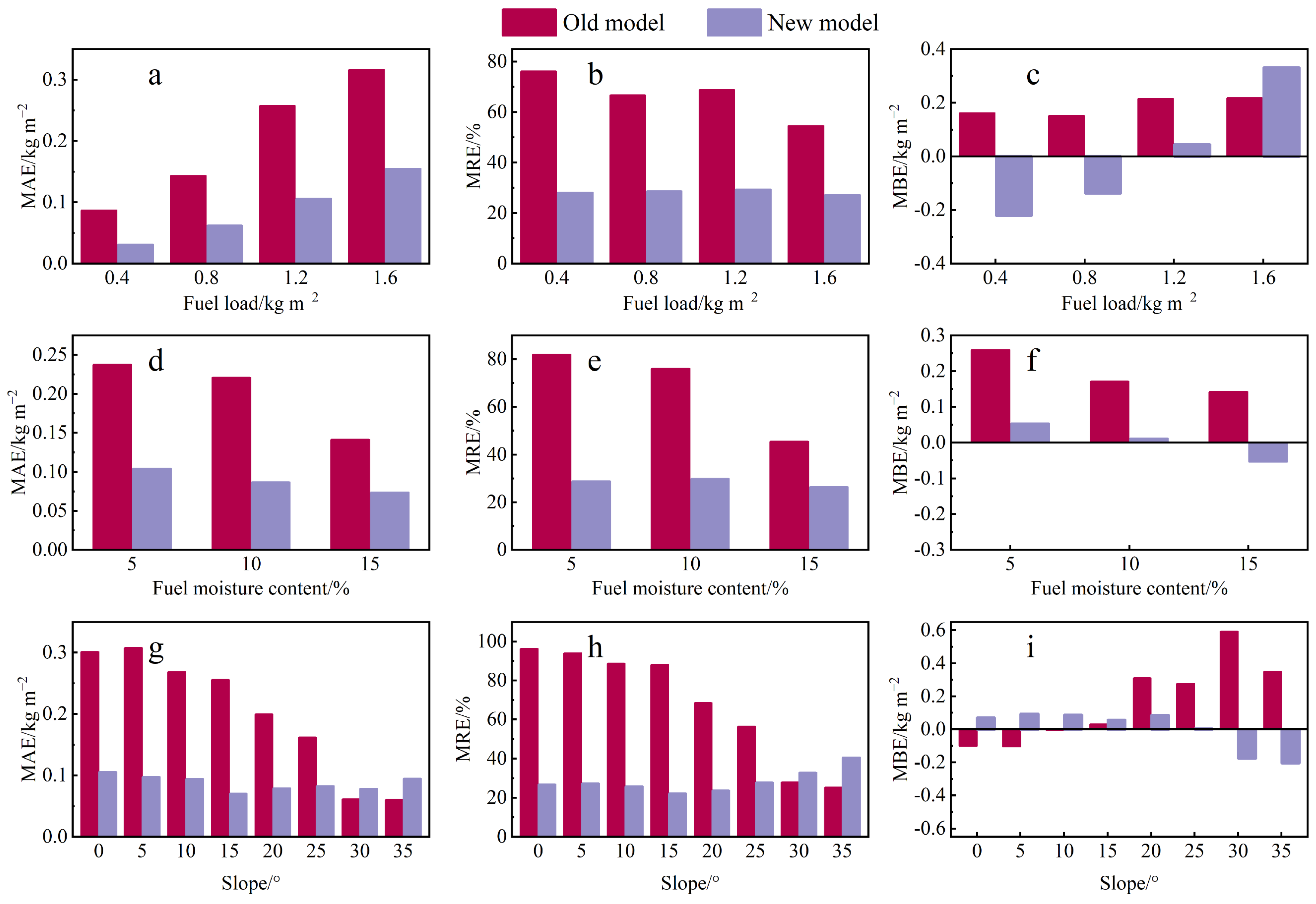
3.3.2. Fuel Carbon Consumption Model Prediction Error

Figure 5 shows the characteristics of the changes in the MAE, MRE, and MBE for different combinations of influencing factors. We can see that the MAE and MRE of the new model are smaller than those of the old model for all conditions, except for the slopes of 30° and 35°, where the MAE and MRE of the new model are larger than those of the old model (Figure 5a,d,g). The MAE values of the new model were reduced by 0.056, 0.081, 0.152, and 0.161 kg m−2 for fuel loadings of 0.4, 0.8, 1.2, and 1.6 kg m−2, respectively (Figure 5a), and the MRE values were reduced by 48.06%, 38.02%, 39.38%, and 27.34%, respectively (Figure 5b), when compared with the values obtained for the old model. The MAE values decreased by 0.134, 0.134, and 0.068 kg m−2, and the MRE values decreased by 53.17%, 46.16%, and 19.02%, respectively, when the fuel moisture contents were 5%, 10%, and 15%. The MAE decreased by 0.195, 0.210, 0.174, 0.185, 0.121, and 0.079 kg m−2 at slopes of 0°, 5°, 10°, 15°, 20°, and 25°, respectively, and the MRE values decreased by 69.38%, 66.69%, 62.93%, 65.74%, 44.74%, and 28.59%, respectively. At 30° and 35° slopes, the MAE values of the new model increased by 0.017 and 0.034 kg m−2, respectively, and the MRE values increased by 4.96% and 15.44%, respectively.
More important than the changes in the MAE and MRE is the regression of the type of error. The change in the type of error can be further analysed based on the change in MBE. Figure 5i shows that the old model underestimates carbon consumption from fuel combustion at slopes of 0° and 5°, provides accurate predictions at a slope of 10°, and overestimates values for other slope angles. The new model underestimated surface fuel combustion carbon consumption at fuel loadings of 0.4 and 0.8 kg m−2, a fuel moisture content of 15%, and slopes of 30° and 35° and overestimated fuel carbon consumption under other conditions. After the parameters were corrected, the MAE and MRE of the new model were significantly lower than those of the old model, and the error of the former model in overestimating surface fuel combustion carbon consumption in Pinus koraiensis plantation forests was largely reduced.

4. Discussion

4.1. Effect of Different Influences on Fire Behaviour Characteristics

The fire behaviour characteristics in this study are influenced by slope, fuel load, and fuel moisture content and show general trends similar to those of forest burning principles. However, we still found several phenomena that are worth exploring. The ROS decreases with the increase in slope for specific fuel load and fuel moisture content conditions. This is because, on the one hand, in the combustion experiments carried out in this study, as the slope increased, the flame gradually shifted from tilting to the rear under horizontal conditions to tilting to the unburned fuel in the front, causing a shift in the mode of heat transfer from the flame to the unburned fuel in the front. Dupuy and Maréchal [43] reported that the radiative heating of the unburned fuel in front of a flame increased as slope steepness increased when the slope was between 0° and 20°, but convection had a cooling effect. Liu et al. [40] noted that natural convection dominated convective cooling under low-slope conditions and was roughly of the same intensity as the radiative heat loss. On the other hand, Rothermel [44] reported that the ROS depends on the fuel bed’s bulk density and the fuel particles’ surface area-to-volume ratio. The ROS decreases for surface fine fuels if the bed compression ratio is below or above the optimum. Therefore, it can be hypothesised that, for the specific fuel load and fuel moisture content conditions set in this study, the increase in convective cooling is greater than the increase in radiant heating with the increase in slope, as influenced by the compression ratio of the fuel bed, and therefore, it manifests as a decrease in the ROS with the increase in slope.
Figure 2 shows that the ROS is inconsistent with the increase in slope; the two do not have a superficial linear relationship. For example, when the fuel load is 1.2 kg m−2, and the fuel moisture content is 5%, the ROS increases by only 3.24 times when the slope increases from 0° to 25° but by 2.19 times when the slope increases from 25° to 30°. Butler and Cook [45] analysed the change rule of the ROS with slope. The authors concluded that heat conduction between fuel particles is the primary heat transfer mechanism under low-slope conditions. As the slope increases, flame radiation utilises the primary heat transfer mechanism, and the sharp increase in the fire ROS at higher slopes is due to the increase in convective heat transfer within and on the surface of the fuel bed. Dupuy and Maréchal [43], from the measurements of fuel bed temperatures and radiative heat flow during upslope fires, reported that flame radiation is the dominant heat transfer mechanism affecting the fire spread process when the slope is between 0° and 20°. At slopes greater than 20°, convective heating induced by the flame curl is responsible for a significant increase in the ROS. Drysdale et al. [46] reported that the critical slope of the heat transfer mechanism transition before a fire occurred was between 15° and 20° in small-scale combustion tests, in which Polymethyl Methacrylate (PMMA) was used as the experimental material. As shown in Figure 2, the critical slope of the heat transfer mechanism transition in this study is between 20° and 25°.
In contrast to the findings of some studies, the fuel moisture content did not significantly facilitate or inhibit fuel consumption. From the principles of forest burning and the observed experimental phenomena, it is clear that, during the spread of surface fires, fuel moisture affects fire behaviour characteristics primarily by influencing the ignition energy of unburned combustibles in front of the flame. When a fuel ignites, the water is first heated to its boiling point and completely evaporated before reaching the ignition temperature [47]. Reid et al. [48] reported that, in forest fires, surface fine fuels generally dry up to the same fuel moisture content level as during the preheating phase before combustion begins. When the fuel ignites, as the flame spreads forward, the latent heat of vaporisation required to evaporate moisture between adjacent fuels absorbs the heat released from fuel combustion. Moreover, the water in the fuel is released into the air as water vapour, which reduces the oxygen concentration [49]. Thus, as the fuel moisture content increases, the ROS, flame length, and fireline intensity decrease. The decrease in the ROS increases the flame residence time, which results in more fuel being consumed. Therefore, at higher fuel moisture content, the fuel burns more completely. Conversely, with a lower fuel moisture content, the ROS is faster, and the flame residence time is shorter, which may result in less fuel consumption. However, in this study’s combustion experiments, it was observed that when the flame was burning at a steady state, the area behind it that was burnt through continued to burn negatively. Therefore, the fuel moisture content did not significantly affect fuel consumption in this study because the fuel consumed in the shadow combustion compensated for the fuel consumed in the open-flame combustion when the fuel moisture content was high. In future studies, we can set a more extensive range of fuel moisture content and smaller intervals to study the effect of the fuel moisture content on fuel consumption.

4.2. Error Analysis of Model Predictions of Fuel Combustion Carbon Consumption

In current forest fire carbon consumption prediction studies, 0.45 g C g−1 is generally used as the amount of carbon contained in surface fuels per unit mass, and surface fuels are assumed to be wholly consumed (i.e., the combustion efficiencies are 100%). However, this study revealed that surface fuel consumption in Pinus koraiensis plantations was not the same under different influencing factors. Even under the most favourable conditions for fuel combustion, fuel was only partially consumed. Fuel consumption varied greatly for different slope conditions, fuel loads, and fuel moisture contents. Ping et al. [29] reported that surface fuels were not fully consumed by fire through the study of different forest fuel types in Northeast China, with combustion efficiencies ranging from 49% to 85%, which is the same as the findings of this study. Peterson et al. [50] reported that variations in fuel consumption depend on many factors, including the structure and arrangement of the fuels (e.g., fuel load, size, surface-to-body ratio), fuel moisture content, slope, and other factors. Fuel consumption varied considerably with different influences. Therefore, setting the combustion efficiency of surface fuels to a constant value (100%) is not appropriate. The carbon content of the Pinus koraiensis plantation surface fuel used in this study was 48.30% (i.e., 0.48 g C g−1), and the ratio of carbon consumption-to-fuel consumption was 0.46. This suggests that the carbon contents of different fuel types vary and that the fuel was not fully consumed over the range of gradients set in this study. Therefore, there is significant uncertainty in the prediction of carbon consumption when 0.45 g C g−1 is used as a constant value [51]. Research on carbon depletion caused by forest fires shows that carbon depletion due to forest fires is currently overestimated if changes in fire severity are excluded [52].
The results of the error analysis of the carbon consumption model for surface fuel combustion in Pinus koraiensis plantation forests revealed that, compared with the old model (which uses the original parameters of the Byram fireline intensity model), the new model (which uses the corrected parameters) had significantly lower mean errors under different combinations of influencing factors and significantly greater prediction accuracy and that the new model reduced the overestimation bias to a large extent. The significant prediction errors of the old model are due to two factors. (1) Different fuel types were used in the old model. The old model used in this study was built by reorganising the Byram fireline intensity model and introducing the ratio of fuel carbon consumption-to-overall fuel consumption, which kept the original parameter values the same. Its essence is still the Byram fireline intensity model. In contrast, the original parameter values (a and b) of the old model were obtained by fitting U.S. fuel combustion data, which differed from those of the fuels used in this study in terms of dimensions (shape, size), particle density, and calorific value. Related studies have shown that changes in fuel type can cause changes in convection and radiation during fuel combustion, causing changes in forest fire behaviour characteristics such as the ROS. Benali et al. [31] noted that small changes in fuel structure might lead to significant changes in predicted or measured fire behaviour. Fernandes et al. [53] and Dupuy et al. [54] conducted indoor and outdoor burning tests and reported that different fuel types corresponded to different values of the parameters of the Byram fire intensity equation. Therefore, this study’s accuracy in predicting the carbon consumption of surface fuels in Pinus koraiensis plantation forests using the old model is low. (2) The old model used coarse fire data. The fire dataset used in the previous model contained variations in fuel types, estimates of fuel types across the landscape, and average wind speeds and slopes at both spatial and temporal scales. This resulted in a coarser fire dataset with significant uncertainty [55]. Fire researchers evaluating the ROS from raw fire datasets have reported that modelled MREs are typically 30%–50% [56,57,58]. Cheney et al. [57] modelled and evaluated fire behaviour models using independent data and reported that the low reliability of forest fire data resulted in model predictions with MAE values more than twice as high as those of reliable data. Thus, the low prediction accuracy of the old model in this study was due to the large-scale uncertainty of the original fire dataset.
The average MAE of the new model is significantly lower than that of the old model. The improved prediction accuracy of the new model is not coincidental. Instead, we achieved this improvement in accuracy through a more rigorous experimental design, including a broader experimental gradient, more precise experimental data, and the use of least squares to correct the model parameters rather than just a form driven by a simple statistical fit [59]. However, noteworthily, the new model still has some errors (i.e., an average MRE of 28.28%), which may be due to its limitations and accuracy. Alexander and Cruz [55] reported that models driven primarily by the ROS and fine fuel moisture content explained 84% of the observed variations in fire behaviour characteristics.
Overall, the new model’s average relative error decreased by 0.110 kg m−2, and the average absolute error decreased by 38.48% when compared with the same values from the old model; these improvements, along with the new model’s R2 = 0.75, showed that the new model’s accuracy in predicting surface fuel combustion carbon consumption in Pinus koraiensis plantation forests was significantly improved. Cruz and Alexander [60] performed an accuracy assessment of the current model using 49 fire datasets (including 7 fuel types and 1278 observations) and reported that an error interval with an MRE of 35% could be considered a reasonable model performance criterion. The new model developed in this study has an MRE = 28.28%. Therefore, this new model can be used to predict surface fuel combustion carbon consumption in Pinus koraiensis plantation forests.

4.3. Model Applications, Limitations, and Improvements

In general, fire researchers have developed fire behaviour models to predict or anticipate the outcomes of certain fire phenomena before they occur. In this study, we first reorganised the Byram fireline intensity model. Then, we incorporated the ratio of fuel carbon consumption to overall fuel consumption to develop the initial version of the surface fuel combustion carbon consumption model. The model parameters were then modified based on the measured ROS, flame length, and other data from the combustion experiments. Finally, a prediction model for the carbon consumption of surface fuel combustion in Pinus koraiensis plantation forests was established, and good prediction results were achieved. Owing to the limitations of the experimental conditions, only one fuel type was used in this study to conduct combustion tests indoors with different slopes, fuel loads, and fuel moisture contents, which differed from actual fires in the wild. Therefore, caution is advised when the model is extended to the field for application. However, this study’s modelling process and ideas can still provide new paths and methods for constructing carbon consumption models that can be applied to various fuels. Given the urgent need to accurately assess carbon emissions from forest fires, future research should utilise a combination of laboratory combustion experiments, prescribed burns, and actual forest fire data [61,62] to enhance carbon consumption modelling and support forest fire planning, training, and strategy development. The model developed in this study is a type of fire behaviour prediction model. The improvement in the predictive ability of fire behaviour models stems primarily from other factors, including more detailed fuel characterisation data and more accurate fuel moisture content predictions [63,64,65], more accurate weather forecasts and simulations of complex terrain, wind speed, and direction, and the integration of fire environment prediction and fire behaviour prediction into software, leading to more accurate model predictions [66,67,68]. Finally, we should further develop and improve forest fire modelling tools to support responses to the challenges and impacts of climate change on forest fires.

5. Conclusions

A total of 288 combustion experiments at different slopes (0°, 5°, 10°, 15°, 20°, 25°, 30°, and 35°), fuel loadings (0.4, 0.8, 1.2, and 1.6 kg m−2), and fuel moisture contents (5, 10, and 15%) were conducted in this study. The fire behaviour characteristics and fuel (fuel ash) carbon content during surface fire combustion were measured, resulting in the development of a prediction model of surface fire combustion carbon consumption and an assessment of model accuracy. We conclude that the slope steepness, fuel load, and fuel moisture content affect surface fire behaviour characteristics and are generally consistent with forest burning principles. However, the interactions of these factors lead to opposite trends in some of the fire behaviour characteristics because the bed packing ratio of the fuel affects the preheating process. In this study, the fuel moisture content did not significantly affect fuel carbon consumption. This is due to the large gradient of fuel moisture content set in this study and the continued shadow combustion of the fuel even after it has been overfired. The direct use of the original Byram fireline intensity surface model parameters (old model) predicted fuel carbon consumption with poor accuracy, and the modification of the model parameters using laboratory-acquired fire behaviour data (new model) significantly improved the model’s accuracy in predicting fuel carbon consumption. In future studies, we will investigate the influence of wind speed on surface fire behaviour and further utilise data from both prescribed and actual forest fires to enhance the accuracy of the new model’s predictions for surface fuel-burning carbon consumption.

Author Contributions

D.G.: Writing—original draft, Methodology, Investigation, Data curation, Formal analysis, Conceptualisation, Funding acquisition. J.N.: Writing—original draft, Methodology, Investigation, Data curation, Formal analysis, Funding acquisition. G.Y.: Methodology, Writing—review and editing, Funding acquisition, Project administration, Conceptualisation. S.M.: Writing—original draft, Investigation. L.W.: Formal analysis, Visualisation. H.Y.: Software, Formal analysis. All authors have read and agreed to the published version of the manuscript.

Funding

This work was funded by the National Natural Science Foundation of China (32371881), Fundamental Research Funds for the Central Universities (2572024AW15, 2572023CT01), Postdoctoral Fellowship Program of China Postdoctoral Science Foundation (GZC20230398).

Institutional Review Board Statement

Not applicable.

Informed Consent Statement

Not applicable.

Data Availability Statement

Data are contained within the article.

Conflicts of Interest

The authors declare that they have no conflicts of interest.

References

  1. Canadell, J.G.; Raupach, M.R. Managing Forests for Climate Change Mitigation. Science 2008, 320, 1456–1457. [Google Scholar] [CrossRef] [PubMed]
  2. Fernández-Martínez, M.; Vicca, S.; Janssens, I.A.; Sardans, J.; Luyssaert, S.; Campioli, M.; Chapin Iii, F.S.; Ciais, P.; Malhi, Y.; Obersteiner, M.; et al. Nutrient Availability as the Key Regulator of Global Forest Carbon Balance. Nat. Clim. Change 2014, 4, 471–476. [Google Scholar] [CrossRef]
  3. Steffen, W.; Rockström, J.; Richardson, K.; Lenton, T.M.; Folke, C.; Liverman, D.; Summerhayes, C.P.; Barnosky, A.D.; Cornell, S.E.; Crucifix, M.; et al. Trajectories of the Earth System in the Anthropocene. Proc. Natl. Acad. Sci. USA 2018, 115, 8252–8259. [Google Scholar] [CrossRef]
  4. Lal, R. Forest Soils and Carbon Sequestration. For. Ecol. Manag. 2005, 220, 242–258. [Google Scholar] [CrossRef]
  5. Canadell, J.G.; Le Quéré, C.; Raupach, M.R.; Field, C.B.; Buitenhuis, E.T.; Ciais, P.; Conway, T.J.; Gillett, N.P.; Houghton, R.A.; Marland, G. Contributions to Accelerating Atmospheric CO2 Growth from Economic Activity, Carbon Intensity, and Efficiency of Natural Sinks. Proc. Natl. Acad. Sci. USA 2007, 104, 18866–18870. [Google Scholar] [CrossRef] [PubMed]
  6. Galik, C.S.; Jackson, R.B. Risks to Forest Carbon Offset Projects in a Changing Climate. For. Ecol. Manag. 2009, 257, 2209–2216. [Google Scholar] [CrossRef]
  7. Just, M.G.; Hohmann, M.G.; Hoffmann, W.A. Invasibility of a Fire-Maintained Savanna–Wetland Gradient by Non-Native, Woody Plant Species. For. Ecol. Manag. 2017, 405, 229–237. [Google Scholar] [CrossRef]
  8. Chang, Y.; Zhu, Z.; Feng, Y.; Li, Y.; Bu, R.; Hu, Y. The Spatial Variation in Forest Burn Severity in Heilongjiang Province, China. Nat. Hazards 2016, 81, 981–1001. [Google Scholar] [CrossRef]
  9. Andela, N.; Morton, D.C.; Giglio, L.; Chen, Y.; Van Der Werf, G.R.; Kasibhatla, P.S.; DeFries, R.S.; Collatz, G.J.; Hantson, S.; Kloster, S.; et al. A Human-Driven Decline in Global Burned Area. Science 2017, 356, 1356–1362. [Google Scholar] [CrossRef]
  10. Van Der Werf, G.R.; Randerson, J.T.; Giglio, L.; Van Leeuwen, T.T.; Chen, Y.; Rogers, B.M.; Mu, M.; Van Marle, M.J.E.; Morton, D.C.; Collatz, G.J.; et al. Global Fire Emissions Estimates during 1997–2016. Earth Syst. Sci. Data 2017, 9, 697–720. [Google Scholar] [CrossRef]
  11. Bowman, D.M.J.S.; Williamson, G.J.; Price, O.F.; Ndalila, M.N.; Bradstock, R.A. Australian Forests, Megafires and the Risk of Dwindling Carbon Stocks. Plant Cell Environ. 2021, 44, 347–355. [Google Scholar] [CrossRef] [PubMed]
  12. Cullen, A.C.; Axe, T.; Podschwit, H. High-Severity Wildfire Potential—Associating Meteorology, Climate, Resource Demand and Wildfire Activity with Preparedness Levels. Int. J. Wildland Fire 2021, 30, 30–41. [Google Scholar] [CrossRef]
  13. Higuera, P.E.; Abatzoglou, J.T. Record-setting Climate Enabled the Extraordinary 2020 Fire Season in the Western United States. Glob. Change Biol. 2021, 27, 1–2. [Google Scholar] [CrossRef]
  14. Jain, P.; Castellanos-Acuna, D.; Coogan, S.C.P.; Abatzoglou, J.T.; Flannigan, M.D. Observed Increases in Extreme Fire Weather Driven by Atmospheric Humidity and Temperature. Nat. Clim. Change 2022, 12, 63–70. [Google Scholar] [CrossRef]
  15. Van Oldenborgh, G.J.; Krikken, F.; Lewis, S.; Leach, N.J.; Lehner, F.; Saunders, K.R.; Van Weele, M.; Haustein, K.; Li, S.; Wallom, D.; et al. Attribution of the Australian Bushfire Risk to Anthropogenic Climate Change. Nat. Hazards Earth Syst. Sci. 2021, 21, 941–960. [Google Scholar] [CrossRef]
  16. Walker, X.J.; Baltzer, J.L.; Cumming, S.G.; Day, N.J.; Ebert, C.; Goetz, S.; Johnstone, J.F.; Potter, S.; Rogers, B.M.; Schuur, E.A.G.; et al. Increasing Wildfires Threaten Historic Carbon Sink of Boreal Forest Soils. Nature 2019, 572, 520–523. [Google Scholar] [CrossRef]
  17. Ndalila, M.N.; Williamson, G.J.; Bowman, D.M.J.S. Carbon Dioxide and Particulate Emissions from the 2013 Tasmanian Firestorm: Implications for Australian Carbon Accounting. Carbon Balance Manag. 2022, 17, 7. [Google Scholar] [CrossRef]
  18. Walker, X.J.; Rogers, B.M.; Veraverbeke, S.; Johnstone, J.F.; Baltzer, J.L.; Barrett, K.; Bourgeau-Chavez, L.; Day, N.J.; De Groot, W.J.; Dieleman, C.M.; et al. Fuel Availability Not Fire Weather Controls Boreal Wildfire Severity and Carbon Emissions. Nat. Clim. Change 2020, 10, 1130–1136. [Google Scholar] [CrossRef]
  19. Zheng, B.; Ciais, P.; Chevallier, F.; Chuvieco, E.; Chen, Y.; Yang, H. Increasing Forest Fire Emissions despite the Decline in Global Burned Area. Sci. Adv. 2021, 7, eabh2646. [Google Scholar] [CrossRef] [PubMed]
  20. Sommers, W.T.; Loehman, R.A.; Hardy, C.C. Wildland Fire Emissions, Carbon, and Climate: Science Overview and Knowledge Needs. For. Ecol. Manag. 2014, 317, 1–8. [Google Scholar] [CrossRef]
  21. Wang, C.; Gower, S.T.; Wang, Y.; Zhao, H. The Influence of Fire on Carbon Distribution and Net Primary Production of Boreal Larix Gmelinii Forests in North-Eastern China. Glob. Change Biol. 2001, 7, 719–730. [Google Scholar] [CrossRef]
  22. Seiler, W.; Crutzen, P.J. Estimates of Gross and Net Fluxes of Carbon between the Biosphere and the Atmosphere from Biomass Burning. Clim. Change 1980, 2, 207–247. [Google Scholar] [CrossRef]
  23. Ward, D.E.; Hao, W.M. Projections of emissions from burning of biomass for use in studies of global climate and atmospheric chemistry. Paper 91-128.4. In Proceedings of the 84th Annual Meeting and Exhibition, Vancouver, BC, Canada, 16–21 June 1991; Air and Waste Management Association: Pittsburgh, PA, USA, 1991. 16p. [Google Scholar]
  24. Ball, R. Regulation of Atmospheric Carbon Dioxide by Vegetation Fires. Clim. Res. 2014, 59, 125–133. [Google Scholar] [CrossRef]
  25. Kurz, W.A.; Dymond, C.C.; White, T.M.; Stinson, G.; Shaw, C.H.; Rampley, G.J.; Smyth, C.; Simpson, B.N.; Neilson, E.T.; Trofymow, J.A.; et al. CBM-CFS3: A Model of Carbon-Dynamics in Forestry and Land-Use Change Implementing IPCC Standards. Ecol. Model. 2009, 220, 480–504. [Google Scholar] [CrossRef]
  26. Ramo, R.; Roteta, E.; Bistinas, I.; Van Wees, D.; Bastarrika, A.; Chuvieco, E.; Van Der Werf, G.R. African Burned Area and Fire Carbon Emissions Are Strongly Impacted by Small Fires Undetected by Coarse Resolution Satellite Data. Proc. Natl. Acad. Sci. USA 2021, 118, e2011160118. [Google Scholar] [CrossRef]
  27. Liu, N. Wildland Surface Fire Spread: Mechanism Transformation and Behavior Transition. Fire Saf. J. 2023, 141, 103974. [Google Scholar] [CrossRef]
  28. Garcia-Hurtado, E.; Pey, J.; Baeza, M.J.; Carrara, A.; Llovet, J.; Querol, X.; Alastuey, A.; Vallejo, V.R. Carbon Emissions in Mediterranean Shrubland Wildfires: An Experimental Approach. Atmos. Environ. 2013, 69, 86–93. [Google Scholar] [CrossRef]
  29. Ping, X.; Chang, Y.; Liu, M.; Hu, Y.; Yuan, Z.; Shi, S.; Jia, Y.; Li, D.; Yu, L. Fuel Burning Efficiency under Various Fire Severities of a Boreal Forest Landscape in North-East China. Int. J. Wildland Fire 2021, 30, 691–701. [Google Scholar] [CrossRef]
  30. Ottmar, R.D. Wildland Fire Emissions, Carbon, and Climate: Modeling Fuel Consumption. For. Ecol. Manag. 2014, 317, 41–50. [Google Scholar] [CrossRef]
  31. Benali, A.; Ervilha, A.R.; Sá, A.C.L.; Fernandes, P.M.; Pinto, R.M.S.; Trigo, R.M.; Pereira, J.M.C. Deciphering the Impact of Uncertainty on the Accuracy of Large Wildfire Spread Simulations. Sci. Total Environ. 2016, 569–570, 73–85. [Google Scholar] [CrossRef]
  32. Cheng, K.; Yang, H.; Tao, S.; Su, Y.; Guan, H.; Ren, Y.; Hu, T.; Li, W.; Xu, G.; Chen, M.; et al. Carbon Storage through China’s Planted Forest Expansion. Nat. Commun. 2024, 15, 4106. [Google Scholar] [CrossRef] [PubMed]
  33. Zhang, X.; Chen, X.; Ji, Y.; Wang, R.; Gao, J. Forest Age Drives the Resource Utilization Indicators of Trees in Planted and Natural Forests in China. Plants 2024, 13, 806. [Google Scholar] [CrossRef]
  34. Ning, J.; Yang, G.; Zhang, Y.; Geng, D.; Wang, L.; Liu, X.; Li, Z.; Yu, H.; Zhang, J.; Di, X. Smoke Exposure Levels Prediction Following Laboratory Combustion of Pinus koraiensis Plantation Surface Fuel. Sci. Total Environ. 2023, 881, 163402. [Google Scholar] [CrossRef]
  35. Goto, Y.; Suzuki, S. Estimates of Carbon Emissions from Forest Fires in Japan, 1979–2008. Int. J. Wildland Fire 2013, 22, 721–729. [Google Scholar] [CrossRef]
  36. Zhang, Y.; Sun, P. Study on the Diurnal Dynamic Changes and Prediction Models of the Moisture Contents of Two Litters. Forests 2020, 11, 95. [Google Scholar] [CrossRef]
  37. Geng, D.; Yang, G.; Ning, J.; Li, A.; Li, Z.; Ma, S.; Wang, X.; Yu, H. Modification of the Rothermel Model Parameters—The Rate of Surface Fire Spread of Pinus koraiensis Needles under No-Wind and Various Slope Conditions. Int. J. Wildland Fire 2024, 33, WF23118. [Google Scholar] [CrossRef]
  38. Guo, Y.; Hu, H.; Hu, T.; Ren, M.; Chen, B.; Fan, J.; Man, Z.; Sun, L. Applying and Evaluating the Modified Method of the Rothermel Model under No-Wind Conditions for Pinus koraiensis Plantations. Forests 2024, 15, 1178. [Google Scholar] [CrossRef]
  39. Li, H.; Liu, N.; Xie, X.; Zhang, L.; Yuan, X.; He, Q.; Viegas, D.X. Effect of Fuel Bed Width on Upslope Fire Spread: An Experimental Study. Fire Technol. 2021, 57, 1063–1076. [Google Scholar] [CrossRef]
  40. Liu, N.; Wu, J.; Chen, H.; Xie, X.; Zhang, L.; Yao, B.; Zhu, J.; Shan, Y. Effect of Slope on Spread of a Linear Flame Front over a Pine Needle Fuel Bed: Experiments and Modelling. Int. J. Wildland Fire 2014, 23, 1087–1096. [Google Scholar] [CrossRef]
  41. Ning, J.; Yang, G.; Liu, X.; Geng, D.; Wang, L.; Li, Z.; Zhang, Y.; Di, X.; Sun, L.; Yu, H. Effect of Fire Spread, Flame Characteristic, Fire Intensity on Particulate Matter 2.5 Released from Surface Fuel Combustion of Pinus koraiensis Plantation—A Laboratory Simulation Study. Environ. Int. 2022, 166, 107352. [Google Scholar] [CrossRef]
  42. Byram, G.M.; Nelson, R.M. The Modeling of Pulsating Fires. Fire Technol. 1970, 6, 102–110. [Google Scholar] [CrossRef]
  43. Dupuy, J.-L.; Maréchal, J. Slope effect on laboratory fire spread: Contribution of radiation and convection to fuel bed preheating. Int. J. Wildland Fire 2011, 2, 289–307. [Google Scholar] [CrossRef]
  44. Rothermel, R.C. A Mathematical Model for Predicting Fire Spread in Wildland Fuels; Intermountain Forest & Range Experiment Station, US Forest Service: Washington, DC, USA, 1972; Volume 115. [Google Scholar]
  45. Butler, B.W.; Cook, W. The Fire Environment—Innovations, Management, and Policy. Conference Proceedings. In Proceedings of the RMRS-P-46CD, Destin, FL, USA, 26–30 March 2007; U.S. Department of Agriculture, Forest Service, Rocky Mountain Research Station: Fort Collins, CO, USA, 2007. 662p; CD-ROM. [Google Scholar]
  46. Drysdale, D.D.; Macmillan, A.J.R.; Shilitto, D. The King’s Cross Fire: Experimental Verification of the ‘Trench Effect’. Fire Saf. J. 1992, 18, 75–82. [Google Scholar] [CrossRef]
  47. Simard, A. The Moisture Content of Forest Fuels—1. A Review of the Basic Concepts; Information Report FF-X-14; Department of Forestry and Rural Development, Forest Fire Research Institute: Ottawa, ON, Canada, 1968. [Google Scholar]
  48. Reid, A.M.; Robertson, K.M.; Hmielowski, T.L. Predicting Litter and Live Herb Fuel Consumption during Prescribed Fires in Native and Old-Field Upland Pine Communities of the Southeastern United States. Can. J. For. Res. 2012, 42, 1611–1622. [Google Scholar] [CrossRef]
  49. Catchpole, W.R.; Catchpole, E.A.; Butler, B.W.; Rothermel, R.C.; Morris, G.A.; Latham, D.J. Rate of Spread of Free-Burning Fires in Woody Fuels in a Wind Tunnel. Combust. Sci. Technol. 1998, 131, 1–37. [Google Scholar] [CrossRef]
  50. Peterson, D.L.; McCaffrey, S.M.; Patel-Weynand, T. Wildland Fire Smoke in the United States: A Scientific Assessment; Springer Nature: Berlin/Heidelberg, Germany, 2022; ISBN 978-3-030-87045-4. [Google Scholar]
  51. McMeeking, G.R. The Optical, Chemical, and Physical Properties of Aerosols and Gases Emitted by the Laboratory Combustion of Wildland Fuels; Colorado State University: Fort Collins, CO, USA, 2008. [Google Scholar]
  52. Veraverbeke, S.; Hook, S.J. Evaluating Spectral Indices and Spectral Mixture Analysis for Assessing Fire Severity, Combustion Completeness and Carbon Emissions. Int. J. Wildland Fire 2013, 22, 707. [Google Scholar] [CrossRef]
  53. Fernandes, P.M.; Botelho, H.S.; Rego, F.C.; Loureiro, C. Empirical Modelling of Surface Fire Behaviour in Maritime Pine Stands. Int. J. Wildland Fire 2009, 18, 698–710. [Google Scholar] [CrossRef]
  54. Dupuy, J.-L.; Maréchal, J.; Portier, D.; Valette, J.-C. The Effects of Slope and Fuel Bed Width on Laboratory Fire Behaviour. Int. J. Wildland Fire 2011, 20, 272–288. [Google Scholar] [CrossRef]
  55. Alexander, M.E.; Cruz, M.G. Evaluating a Model for Predicting Active Crown Fire Rate of Spread Using Wildfire Observations. Can. J. For. Res. 2006, 36, 3015–3028. [Google Scholar] [CrossRef]
  56. Anderson, W.R.; Cruz, M.G.; Fernandes, P.M.; McCaw, L.; Vega, J.A.; Bradstock, R.A.; Fogarty, L.; Gould, J.; McCarthy, G.; Marsden-Smedley, J.B.; et al. A Generic, Empirical-Based Model for Predicting Rate of Fire Spread in Shrublands. Int. J. Wildland Fire 2015, 24, 443. [Google Scholar] [CrossRef]
  57. Cheney, N.P.; Gouldl, J.S.; Catchpole, W.R. Prediction of Fire Spread in Grasslands. Int. J. Wildland Fire 1998, 8, 1–13. [Google Scholar] [CrossRef]
  58. Cheney, N.P.; Gould, J.S.; McCaw, W.L.; Anderson, W.R. Predicting Fire Behaviour in Dry Eucalypt Forest in Southern Australia. For. Ecol. Manag. 2012, 280, 120–131. [Google Scholar] [CrossRef]
  59. Cruz, M.G.; Alexander, M.E.; Sullivan, A.L. Mantras of Wildland Fire Behaviour Modelling: Facts or Fallacies? Int. J. Wildland Fire 2017, 26, 973–981. [Google Scholar] [CrossRef]
  60. Cruz, M.G.; Alexander, M.E. Uncertainty associated with model predictions of surface and crown fire rates of spread. Environ. Model. Softw. 2013, 47, 16–28. [Google Scholar] [CrossRef]
  61. Cruz, M.G.; Gould, J.S.; Kidnie, S.; Bessell, R.; Nichols, D.; Slijepcevic, A. Effects of Curing on Grassfires: II. Effect of Grass Senescence on the Rate of Fire Spread. Int. J. Wildland Fire 2015, 24, 838–848. [Google Scholar] [CrossRef]
  62. Perrakis, D.D.B.; Lanoville, R.A.; Taylor, S.W.; Hicks, D. Modeling Wildfire Spread in Mountain Pine Beetle-Affected Forest Stands, British Columbia, Canada. Fire Ecol. 2014, 10, 10–35. [Google Scholar] [CrossRef]
  63. Little, K.; Graham, L.J.; Kettridge, N. Accounting for Among-Sampler Variability Improves Confidence in Fuel Moisture Content Field Measurements. Int. J. Wildland Fire 2023, 33, WF23078. [Google Scholar] [CrossRef]
  64. Pimont, F.; Parsons, R.; Rigolot, E.; De Coligny, F.; Dupuy, J.-L.; Dreyfus, P.; Linn, R.R. Modeling Fuels and Fire Effects in 3D: Model Description and Applications. Environ. Model. Softw. 2016, 80, 225–244. [Google Scholar] [CrossRef]
  65. Sullivan, A.L.; Matthews, S. Determining Landscape Fine Fuel Moisture Content of the Kilmore East ‘Black Saturday’ Wildfire Using Spatially-Extended Point-Based Models. Environ. Model. Softw. 2013, 40, 98–108. [Google Scholar] [CrossRef]
  66. Forthofer, J.M.; Butler, B.W.; Wagenbrenner, N.S. A Comparison of Three Approaches for Simulating Fine-Scale Surface Winds in Support of Wildland Fire Management. Part I. Model Formulation and Comparison against Measurements. Int. J. Wildland Fire 2014, 23, 969–981. [Google Scholar] [CrossRef]
  67. Lopes, A.M.G.; Ribeiro, L.M.; Viegas, D.X.; Raposo, J.R. Effect of Two-Way Coupling on the Calculation of Forest Fire Spread: Model Development. Int. J. Wildland Fire 2017, 26, 829–843. [Google Scholar] [CrossRef]
  68. Plucinski, M.P.; Sullivan, A.L.; Rucinski, C.J.; Prakash, M. Improving the Reliability and Utility of Operational Bushfire Behaviour Predictions in Australian Vegetation. Environ. Model. Softw. 2017, 91, 1–12. [Google Scholar] [CrossRef]
Figure 1. Diagram of the experimental device.
Forests 16 00726 g001
Figure 2. Characteristics of fire behaviour characteristics for different influencing factors: (a) fuel load = 0.4 kg m−2; (b) fuel load = 0.8 kg m−2; (c) fuel load = 1.2 kg m−2; and (d) fuel load = 1.6 kg m−2.
Forests 16 00726 g002
Figure 3. Characteristics of fuel consumption and fuel carbon consumption under different influencing factors: (a) fuel load = 0.4 kg m−2; (b) fuel load = 0.8 kg m−2; (c) fuel load = 1.2 kg m−2; (d) fuel load = 1.6 kg m−2; and (e) fuel consumption in relation to carbon consumption.
Forests 16 00726 g003
Figure 4. Comparison of measured fuel carbon consumption and model predictions. (a) Comparison of predicted and observed values from the new and old models. The dashed line around the line of perfect agreement indicates the ± 35% error interval. (b) Old model predictions fitted to observations (c) New model predictions fitted to observations.
Forests 16 00726 g004
Figure 5. Variation in error with different influencing factors. (ac) are the variations in MAE, MRE, and MBE with fuel loads; (df) are the variations in MAE, MRE, and MBE with fuel moisture content; (gi) are the variations in MAE, MRE, and MBE with slope.
Forests 16 00726 g005
Table 1. Preliminary information for sample plot.
Stand InformationMaximum ValueMinimum
Value
Mean ValueStandard Deviation
Diameter at breast height/cm21.815.318.92.3
Tree height/m14.69.712.21.3
Crown length/m8.64.66.51.4
Crown width/m2.91.72.20.4
Density/N hm−21633.0650.01064.8329.5
Fuel load/kg m−21.50.51.00.3
Table 2. Basic statistics of experimental data.
VariableMean ValueMinimum VALUEMaximum ValueStandard DeviationPercentiles
255075
Preset fuel moisture content/%10.005.0015.004.095.0010.0015.00
Actual fuel moisture content/10010.493.8919.134.115.7310.4814.99
Fuel bed depth/cm4.972.039.171.923.055.006.51
ROS/m min−10.550.112.960.490.250.360.68
Flame length/cm58.328.08136.2525.0138.0058.5072.00
Fuel consumption/kg m−20.7250.2201.3890.3760.3270.6941.020
Fireline intensity/kW m−1160.1712.011158.74185.7446.7796.02195.68
Fuel carbon consumption/kg m−20.3140.0850.6520.1730.1390.2820.439
Disclaimer/Publisher’s Note: The statements, opinions and data contained in all publications are solely those of the individual author(s) and contributor(s) and not of MDPI and/or the editor(s). MDPI and/or the editor(s) disclaim responsibility for any injury to people or property resulting from any ideas, methods, instructions or products referred to in the content.

