Article

Quantification of the Influencing Factors of Stand Productivity of Subtropical Natural Broadleaved Forests in Eastern China Using an Explainable Machine Learning Framework

1
Zhejiang Forest Resource Monitoring Center, Hangzhou 310020, China
2
School of Forestry and Biotechnology, Zhejiang A & F University, Hangzhou 311300, China
3
Zhejiang Forestry Survey Planning and Design Co., Ltd., Hangzhou 310020, China
4
East China Inventory and Planning Institute, State Forestry and Grassland Administration, Hangzhou 310019, China
*
Author to whom correspondence should be addressed.
Forests 2025, 16(1), 95; https://doi.org/10.3390/f16010095
Submission received: 23 November 2024 / Revised: 23 December 2024 / Accepted: 3 January 2025 / Published: 8 January 2025
(This article belongs to the Special Issue The Relationship between Biomass Growth and Tree Size)

Abstract

:
Natural broadleaf forests (NBFs) are the most abundant zonal vegetation type in subtropical regions. Understanding the mechanisms influencing stand productivity in NBFs is important for developing “nature-based” solutions for climate change mitigation. However, minimal research has captured the effects of nonlinearities and feature interactions that often have nonlinear impacts on stand productivity and influencing factors. To address this research gap, we used continuous forest inventory data, and a machine learning model for stand productivity of NBFs was constructed. Subsequently, through leveraging the interpretable machine learning framework of the SHapley Additive explanation (SHAP) and partial dependence plot, we determined global and local explanations of the influencing factors of stand productivity. Our findings indicate the following: (1) The Autogluon model performed the strongest based on R2, RMSE, and rRMSE metrics. (2) The basal area (BA), neighborhood comparison of diameter at breast height (NC), and stand age (AGE) were the key influencing factors. Stand productivity increased with increasing BA and decreased with increasing NC and AGE. BA was maintained above 15 m2ha−1 and NC was maintained below 0.45, which represent favorable conditions for NBFs to maintain optimal growth. (3) SHAP interaction values were calculated to determine the effects of the five major interactions on stand productivity. Our study provides a reference for the sustainable management of NBFs, thereby highlighting the important role of forests in mitigating climate change.

1. Introduction

Forests are the most important terrestrial ecosystem, and stand productivity, a fundamental feature of their community structure, plays a central role in global carbon dynamics [1]. Crow et al. [2] defined stand productivity as the accumulation of wood production over a certain period. Mamo and Sterba [3] defined the term as the productive capacity of a particular species at a particular site in its natural environment. Herraiz et al. [4] considered stand production to represent the amount of change in aboveground biomass over time. Stand production also has the potential to sustain tree growth in terms of climate, topography, soil, and vegetation [5]. In summary, stand productivity provides comprehensive information on environmental and stand factors. An increase in stand productivity indicates an increase in forest ecosystem services and timber production capacity [6]. Thus, determining the mechanisms by which the influencing factors and interactions affect stand productivity is crucial.
Scholars have attempted to reveal the influential mechanisms of forest productivity at different scales, such as in global [7], national-scale pine- [8], and oak-dominated broadleaf forests [9], subtropical fir forests [10], and nature reserve-scale [11], small mountainous area-scale pine [12], and mixed fir–pine–beech forests [12]. Previous studies have also examined the effects of various factors on stand productivity. In terms of exogenous variables, temperature and precipitation are widely recognized as the most consequential influencing factors, as they alter gas exchanges and water transport through their effects on functional traits [13,14]; these alterations, in turn, affect forest growth. However, the effect of climate on stand productivity varies according to forest type [15]. Recently, bioclimatic variables have been incorporated into stand productivity prediction models [7,16]. The topography is closely related to soil fertility and light conditions and strongly influences the spatial variability of forest productivity [17]. In terms of endogenous factors, several studies have noted that stand productivity is closely related to species diversity and that greater species richness contributes to increases in stand productivity [18,19,20]. Stand productivity tends to decrease with increasing stand age, and stand age also influences the proportion of forest biomass distributed among different components [21]. Size inequality or spatial heterogeneity can lead to differences in resource acquisition and competition intensity among trees, thereby affecting stand productivity [22]. Basal area (BA) is the most important factor affecting stand productivity, with a predominantly negative effect; however, a positive effect also exists [23]; this is because both increasing and decreasing possibilities of complementary effects exist as BA increases [24,25], depending on whether the strength of the complementary effect is greater than that of the competition [22]. Uncertainty currently exists regarding the positivity and negativity of BA effects, however. Further research is required on additional forest types and regions.
Various research methods have been used to quantify these influencing factors, including correlation analysis [26], linear regression models [27,28], and structural equation modeling [27,28]. Recently, machine learning (ML) algorithms have been used to improve model prediction performance owing to their ability to model complex nonlinear relationships with a high accuracy and without strict restrictions on the type, distribution, and number of input variables. ML is considered a powerful modeling tool for predicting forest growth [29]. Scholars are interested in adopting ML algorithms and incorporating ante or post hoc elucidation techniques to explore the complex influencing mechanisms of the stand carbon sequestration potential [30], site index [5], and stand productivity [10]. Each ML model has strengths, and the most appropriate model is not known in advance. Therefore, constructing multiple ML models and selecting the best option may prove more effective than selecting and using a particular model directly.
In summary, although extensive and integral studies have been conducted on the mechanisms influencing stand productivity, considerable room for improvement remains. First, few studies have been conducted on broadleaf forests, especially natural broadleaf forests (NBFs), and the mechanisms influencing stand productivity remain unclear. Second, existing methods focus on the analysis of linear relationships and fail to capture the effects of nonlinearities and feature interactions that often have nonlinear effects between stand productivity and influencing factors [19,31,32]. Finally, the variable importance ranking, which identifies the importance of influencing factors, does not reveal the positive and negative effects of the variables or the local mechanisms in each sample. Local interpretable model-agnostic explanation and partial dependence plot (PDP) algorithms have been applied to ML models to explain the mechanisms of variables affecting prediction results; however, these two methods are less concerned with global interpretability.
Broadleaf forests in the subtropics are a forest type endemic to the same latitudes worldwide. Among them, the NBF has the most stable community structure and plays an important role in ecosystem services. According to the 9th Continuous Forest Inventory (CFI), China’s broadleaf forests cover an area of 103.85 million km2 (57.6% of forests), of which NBFs account for 74.0%. Therefore, the role of NBFs in the accumulation of forest biomass and maintenance and provision of ecosystem services should be evaluated. Natural forests in subtropical China have recently been included as national natural forest protection areas, and their protected area is expected to continue to increase. Therefore, it is necessary to understand the mechanisms influencing NBF stand productivity.
The aims of our study were to (1) determine the stand productivity prediction performance of different ML models and determine whether their performance was superior to the linear regression model; (2) provide global and local explanations of drivers and understand key factors and nonlinear effects; and (3) capture how key interactions affect stand productivity.

2. Materials and Methods
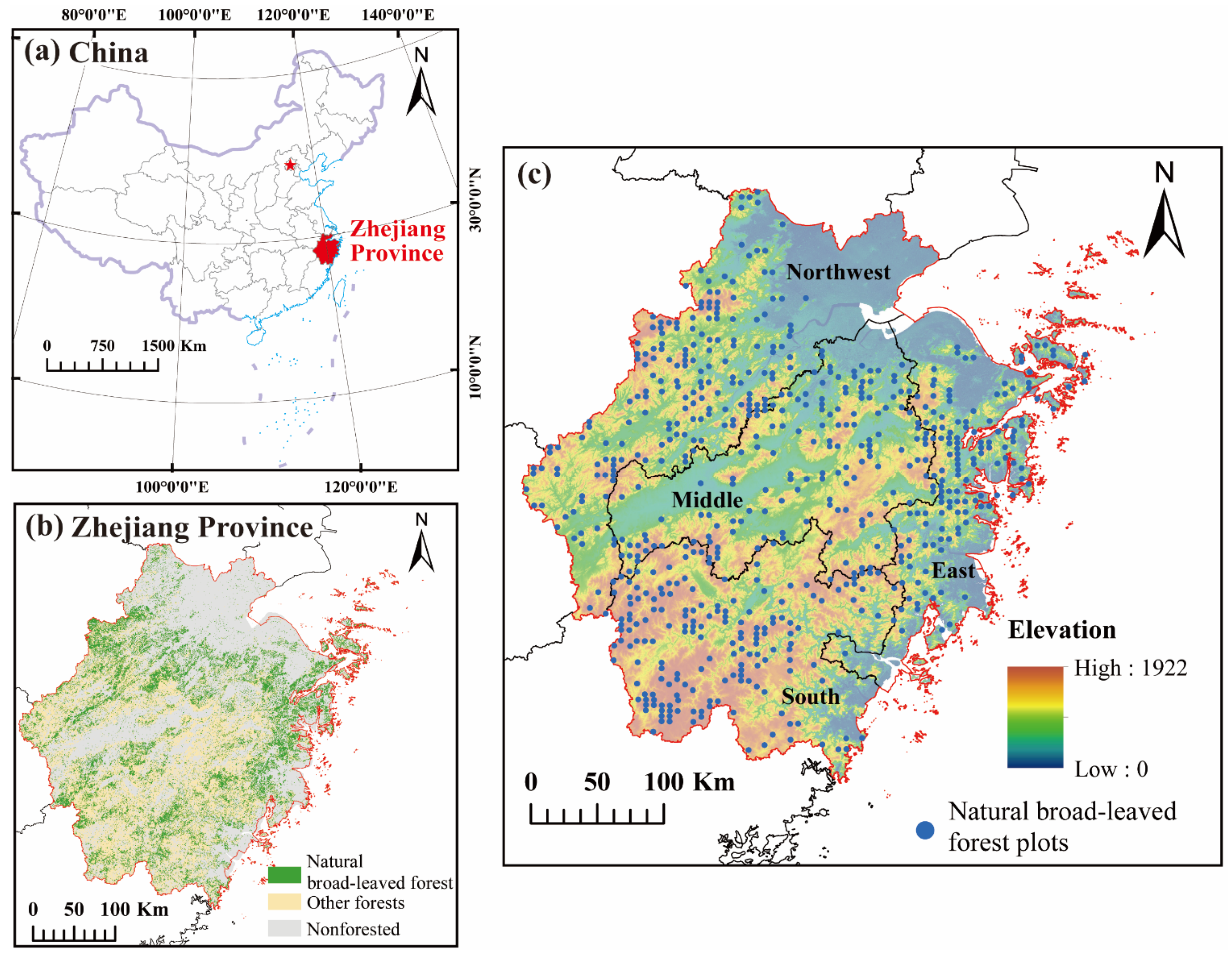
In this study, we established an explainable ML framework by selecting the optimal-performance ML model and incorporating the SHapley Additive explanation (SHAP) and PDP approaches. Data from 642 NBF plots in Zhejiang Province, China, were used to study the influential patterns of stand productivity. Although this framework has been widely used in the fields of medicine [33], the chemical industry [34], and urban studies [35], it has not been utilized to explain the influencing mechanisms of stand productivity.

2.1. Study Area

Zhejiang Province is located on the southeastern coast of China, in the subtropical monsoon humid climate zone, with an annual rainfall of 980–2000 mm and an average annual temperature of 15–18 °C. The province spans 105,500 km2 and comprises approximately 70% hilly mountains. The southwestern part is mountainous, with an average elevation of more than 1000 m. The central part is mostly hilly, with an elevation of less than 500 m, whereas the northeastern part is an alluvial plain with an elevation of less than 10 m. The 9th CFI shows that the forested area of Zhejiang Province was estimated to be 42,688 km2, of which the NBF area comprises 16,448 km2. The province’s tree species mainly include Schima superba, Quercus glauca, Lithocarpus glaber, and Quercus fabri.

2.2. Data Collection and Processing

2.2.1. Stand Productivity Calculation

A total of 642 CFI plots that included NBFs in both 2014 and 2019 and which did not experience major human disturbances were used in this study (Figure 1c). Every plot had dimensions of 28.28 × 28.28 m. Fixed stakes were buried in the northwest corner of the plots. The plots were inventoried from May each year, and each normally growing tree with a diameter at breast height (DBH) ≥5 cm in the plots was hung with a fixed numbered aluminum tag and surveyed for attributes (including species, DBH, and coordinates). The harvested, standing dead, and fallen trees found in the 2019 inventory retained their original numbers and had a DBH equal to that of the 2014 inventory. A one-way volume model [36] was used to calculate the individual tree stem volumes (Equation (1)) and then summed to obtain the stand volume.
V = a a 1 + b 1 D b a 2 + b 2 a 1 + b 1 D + k c
where D is DBH (cm), and a1, b1, a2, b2, k, a, b, and c are parameters (see Table S1). In constructing the one-way volume model, Zhejiang Province was divided into four regions: northwestern, central, eastern, and southern, ensuring that the values of a2, b2, and k were matched according to the region where the plots were located.
Following the method (Equation (2)) of Liang et al. [7], stand productivity (SP, m3ha−1year−1) was measured as the tree volume productivity in terms of periodic annual increment.
S P = 1 t i = 1 n V i , 2019 i = 1 n V i , 2014 + D T A
where Vi,2014 and Vi,2019 represent the total stem volume (m3) of an ith alive tree in 2014 and 2019, respectively; DT constitutes the total volume (m3) of dead trees, including the volume of harvest and mortality during the interval [7]. For trees that were standing trees in the first inventory but were harvested during the interval, or were dead standing trees in the second inventory, the DBH measured in the first inventory was used to calculate the tree stem volume, which was used as the volume of harvest and mortality, respectively; t denotes the time interval between the two inventories (i.e., 5 years), and A represents the plot area (i.e., 0.08 ha).

2.2.2. Influencing Factor Data

The explained variable in this study was stand productivity, and the influencing factors (i.e., explanatory variables) were selected based on stand, topography, and climatic conditions. The stand conditions included the stand age (AGE), basal area (BA), Simpson index (SIMP), neighborhood comparison of DBH (NC), and angular scale index (ASI), which indicate stand density, species diversity, structural diversity, and spatial distribution diversity, respectively. The equations for BA, SIMP, NC, and ASI are shown in the Supplementary Materials. The stand age in the study area was determined as follows: Firstly, the average DBH of the NBF was calculated from the field survey. Secondly, the tree consistent with that average DBH was found within the stand and its age was visually measured. Finally, this tree age was used as the NBF stand age. NC quantifies size inequality from a spatial structure perspective, considering the relative differences between the central and neighboring trees. This is not possible with diameter distribution statistics [37], especially when trees of the same order of diameter are distributed in separate aggregates. Previous studies have indicated that size inequality is closely related to stand growth [23]. Topographic conditions were reflected by slope (SLOP), elevation (ELEV), and aspect (ASPE). With reference to Liang et al. [7], climate conditions included the mean annual temperature (AMT), annual precipitation (AP), isothermality (ISOT), temperature seasonality (TS), and precipitation of the warmest quarter (PWQ). Temperature seasonality is the standard deviation of monthly temperatures multiplied by 100. Isothermality is expressed as the mean of the monthly Max temperature minus the Min temperature, divided by the difference between the Max temperature of the warmest month and the Min temperature of the coldest month [38].
The calculation methods for BA, SIMP, NC, and ASI are provided in the Supplementary Materials. Raster data for the digital elevation model (DEM) and bioclimatic variables were obtained from the Earth Data (https://www.earthdata.nasa.gov, accessed on 18 February 2024) and WorldClim (https://www.worldclim.org, accessed on 16 February 2024) sites, respectively. The geographic and meteorological conditions of the plots were obtained using the “multi-value extraction to points” tool in ArcGIS 10.8 software. The slopes were categorized as shady (337.5–67.5°), semi-shady (67.5–112.5° and 292.5–337.5°), semi-sunny (112.5–157.5° and 247.5–292.5°), and sunny (157.5–247.5°), and expressed as 1, 2, 3, and 4 discrete variables, respectively. Descriptive statistics of the data are shown in Table 1.

2.2.3. Influencing Factor Screening Based on Boruta’s Algorithm

The random forest (RF)-based Boruta’s algorithm was used for feature variable screening. Boruta’s algorithm first randomly sorts the original features to form shadow features and then combines the original features to form an extended database. Second, the RF model was executed on the extended data and the Z-score for each influencing factor was calculated by dividing the mean accuracy loss by its standard deviation. Finally, the maximum Z-score (MZSA) was determined and the Z-score of each original feature was compared with that of the MZSA. If Z-score > MZSA, the feature was retained; otherwise, it was rejected. Boruta’s algorithm was implemented in the R package “Boruta 8.0.0”. The parameters mtry, ntree, and maxRun were set to 5, 600, and 500, respectively.

2.3. Machine Learning Models

The commonly used individual ML models, RF, gradient boosting regression (GBR), eXtreme Gradient Boosting (XGBoost), categorical feature gradient boosting (CatBoost), light gradient boosting machine (Light GBM), and support vector regression (SVR), were selected to construct the stand productivity prediction model. Stacking and voting ensemble methods were used to ensemble individual ML models. Ensemble learning methods reduced model variance by combining the predictions of multiple single ML models. However, if the performance of an individual ML model was the same as or superior to that of an ensemble model, the individual ML model was used because it was less complex. We also used the Autogluon-Tabular model (Autogluon model abbreviation used below), which is an open-source library of the Auto ML framework for structured data designed by Amazon [39]. As an AutoML framework, the Autogluon model combines ML algorithms based on multilayer stacking and repeated k-fold bagging techniques, and is a powerful model integration. This model is also capable of autonomously selecting the best hyperparameters during model training, thereby reducing overfitting risk. The Autogluon model has been used as the optimal model in studies on landslide hazards [40], biogas performance [41], and soil greenhouse gas emissions [42]. The ML models are presented in the Supplementary Materials. In addition, we also constructed a linear regression (LR) model and evaluated the model performance, analyzing the significance and contribution of each variable using the “glmm.hp” R package (version 0.1-2) [43]. These results serve as benchmarks to help better understand the performance of ML models.
Hyperparameters were optimized using the randomized search method. The hyperparameter optimization ranges and results for each model are presented in Tables S2 and S3, respectively. The stacking and voting ensemble ML models were trained using each model’s optimal hyperparameters. The Autogluon model was trained using default parameters. ML model training and hyperparameter optimization were based on the scikit-learn 1.3.2, catboost 1.2.2, and autogluon 1.1.0 python packages, and were implemented in the PyCharm (version 17.0.9) integrated development environment (IDE) via the Python language (version 3.10). The coefficient of determination (R2), RMSE, and relative root mean square error (rRMSE) calculated by a 5-fold cross-validation were used to evaluate the model performance using the following equations:
R 2 = 1 i = 1 n y i r e a l y i p r e d 2 i = 1 n y i r e a l y m e a n r e a l 2
R M S E = i = 1 n y i r e a l y i p r e d 2 n
r R M S E = R M S E y ¯ × 100 %
where y i r e a l is the actual observed value, y i p r e d is the model-estimated value, y m e a n r e a l is the mean actual observed value, and n is the number of samples. To avoid the influence of the sample order on the cross-validation results, we used the shuffle method to split the data and set a fixed random seed, which ensured the consistency of this method when splitting the datasets over multiple experiments.

2.4. SHAP (Shapley Additive Explanation) Algorithm

Because ML models approximate a black box, their interpretability is difficult. The goal of an interpretable ML is to understand how models make predictions [44], including which feature variables have the strongest effects on predictions and the relationship between the input values of the feature variable and the final output values of the model. In a recent study, ML models based on the SHAP theory were widely used. The SHAP theory is an extension of the concept of the Shapley value in game theory [45], and aims to fairly distribute the respective contributions of participants when they collectively reach an outcome. The SHAP value also determines the threshold for each variable [46]. SHAP values were previously calculated with the “shap” Python package developed by Lundberg and Lee [47]. The SHAP value (Equation (6)) of a feature represents its marginal contribution to the model prediction averaged over all possible models with different combinations of features.
S h a p l e y X i = S F \ i S ! n S 1 ! n ! f S i f S
where Shapley (Xi) is the SHAP value of influencing factor Xi, F \ i is the set of all possible combinations of features, excluding Xi, S is the feature set in F \ i , and n is the total number of features. S ! n S 1 ! / n ! denotes the weight, f (S) constitutes the model prediction with features in S, and f S i represents the model prediction with features in S and Xi.

3. Results

3.1. Importance Analysis Screening of Influencing Factors

Figure S1 shows the Z-scores of the influencing factors obtained using the Boruta algorithm. For the stand productivity dataset of the study area, ASPE was labeled as the rejected variable, and the rest were deemed important variables. Among the retained variables, BA had the highest mean Z-score and SLOP had the lowest mean Z-score, at 48.6535 and 2.6158, respectively. Variable importance was categorized into low (<5), medium (5–10), and high (>10) levels, according to the mean Z-score. BA, NC, AGE, and ASI were high; AMT, ISOT, ELEV, and PWQ were moderate; and TS, AP, SIMP, and SLOP were low. On this basis, the variance inflation factor (VIF) was used to test for multicollinearity (results are shown in Table S4). After excluding PWQ variables with a high VIF, 11 influencing factors were ultimately determined.

3.2. Forecasting Performances of Machine Learning Models

Based on the RMSE values (Table 2; see Figure S2 for scatter plots), the individual ML model performances ranked highest to lowest were RF, SVM, Light GBM, CatBoost, GBR, and XGBoost (the hyperparameter optimization ranges and optimization results are shown in Tables S2 and S3, respectively). The best-performing RF was used as a metamodel for the stacking ensemble model for the prediction model. The results show that the voting ensemble model performs slightly better than the stacking ensemble model and outperforms the single ML model. The RF and SVM performances were superior to those of the stacking ensemble model. Compared to the RF, the Autogluon model had reduced RMSE and rRMSE values, by 0.0434 m3ha−1year−1 and 0.9016%, respectively, and an improved R2, by 0.0276. We also built a linear regression (LR) model for comparison with the ML model; only XGBoost performed worse than LR.

3.3. Model Interpretability Analysis

3.3.1. Global and Local Model Interpretability

An interpretability analysis of the best-performing Autogluon model using the SHAP theory was performed. Figure 2a shows the global characteristic importance of each factor on stand productivity. The mean absolute SHAP value of each factor was ranked from high to low, and the closer it was to the top, the greater its influence on stand productivity. The top three influencing factors were BA, NC, and AGE, which accounted for 73.04% of the mean absolute SHAP values.
To more comprehensively explain the effects of each influence on stand productivity, localized effects were observed using SHAP summary plots (Figure 2). Positive SHAP values indicated a positive relationship between stand productivity and drivers, whereas negative values indicated a negative relationship. To clarify these relationships, we constructed a stand productivity forecasting model rather than a causality model. Therefore, positive or negative SHAP values do not imply a causal relationship. BA had the strongest effect on stand productivity; in Figure 2b, the red dots are mainly on the right side of the y-axis, indicating that stand productivity increased with increasing BA. NC and AGE had the second-highest and third-highest effects on stand productivity, respectively; the red dots for these factors were located on the left side of the y-axis (Figure 2b), indicating that stand productivity tended to decrease when the NC and AGE values were higher. ISOT, AMT, ASI, and SLOP were equally important; however, ISOT and AMT were positively correlated with stand productivity, whereas ASI and SLOP were negatively correlated. AP, ELEV, SIMP, and TS had few effects on stand productivity in this study.
The results (Table S6) for the significance and contribution of variables based on the LR model also showed that the model R2 was 0.4179 (this is the fitted R2 and not the validated R2 as above), and the F-statistic was 41.12 (p < 0.0001, with 630 degrees of freedom). Seven variables, BA, NC, and AGE, had significant effects on stand productivity. We found that (1) only the variables with the top seven absolute SHAP values were significant, among which the combined contribution of BA, NC, AGE, and ASI was 90.73%, indicating that stand characteristics were dominant in affecting NBF stand productivity; (2) although there were some differences in the order of the contribution rates of the variables between the two models, the contribution rates of the significant variables were all ranked in the top seven.

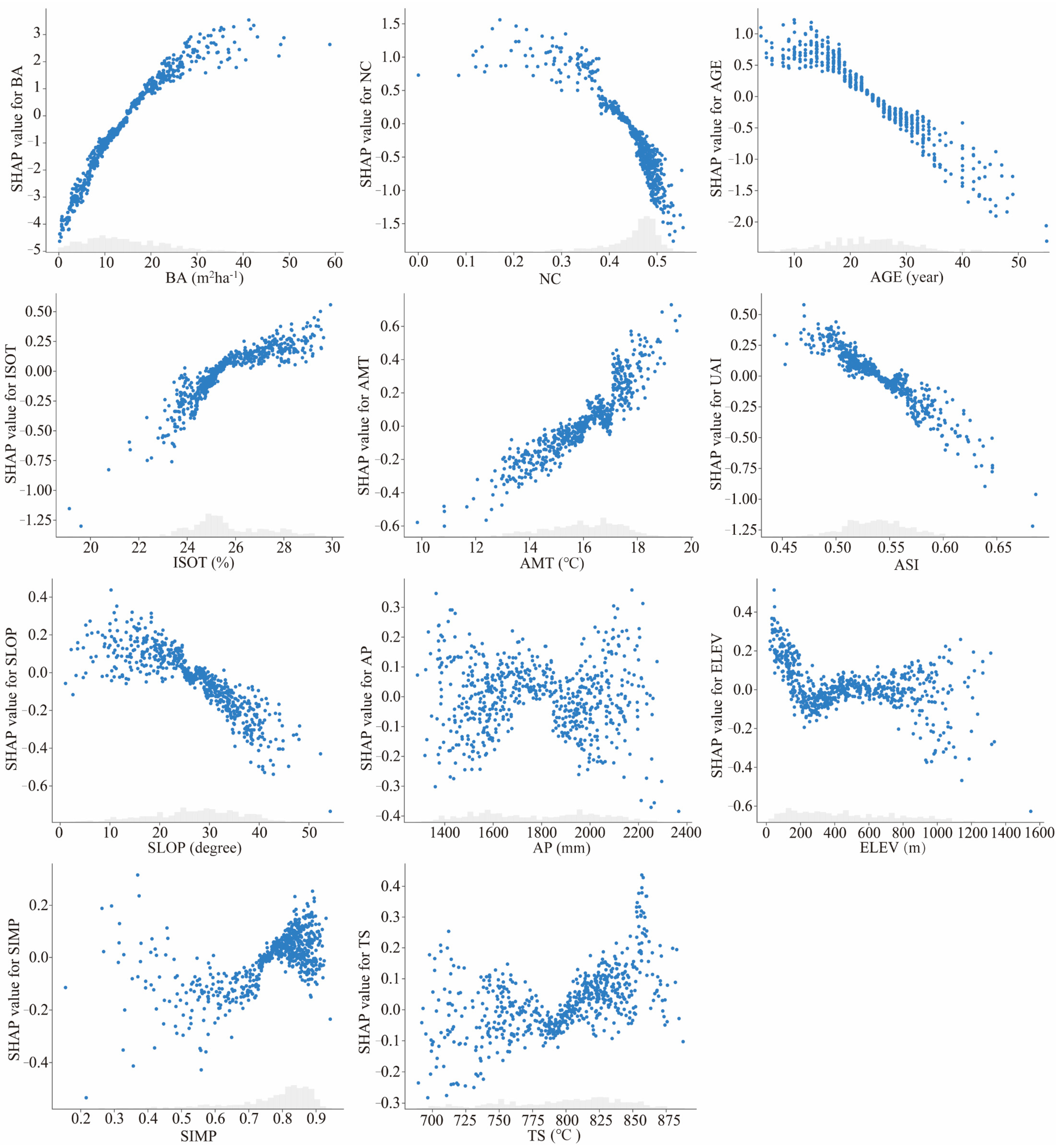
3.3.2. Factor Dependence Analysis

We created SHAP dependence plots (Figure 3) to characterize how SHAP values vary with driver values. Taking the driver value when the SHAP value was 0 as the boundary, the variables had opposite effects on stand productivity. Among the three important factors, when BA < 15 m2ha−1, the SHAP values and BA were negatively correlated, implying a negative contribution of BA to stand productivity forecasting. Similarly, when NC > 0.44, stand productivity did not increase. Moreover, when NC > 0.38, the decline in SHAP values became faster with an increase in NC. There was a negative correlation between AGE and SHAP values, and their contribution to increasing stand productivity decreased with increasing stand age. AGE > 25 provided a more negative contribution to stand productivity.
Both ISOT and AMT showed a negative to positive contribution to stand productivity, with thresholds of 25 and 16 °C, respectively. With an increase in the variable values, the contributions of ASI and SLOP to the predicted value of stand productivity changed from positive to negative, with thresholds of 0.54 and 28°, respectively. However, the effects of AP were unstable. Increases and decreases in annual precipitation drove increases or decreases in stand productivity. When ELEV < 300 m, its contribution to the forecasting results was positive. When the ELEV was between 300 and 800 m, its effect on stand productivity was relatively stable, with both positive and negative contributions occurring simultaneously. When ELEV > 800 m, the effect became unstable. The SIMP threshold was 0.80, and both positive and negative contributions were present at a SIMP > 0.80. When TS < 8 °C, its effect on stand productivity was unstable; conversely, a positive contribution dominated.

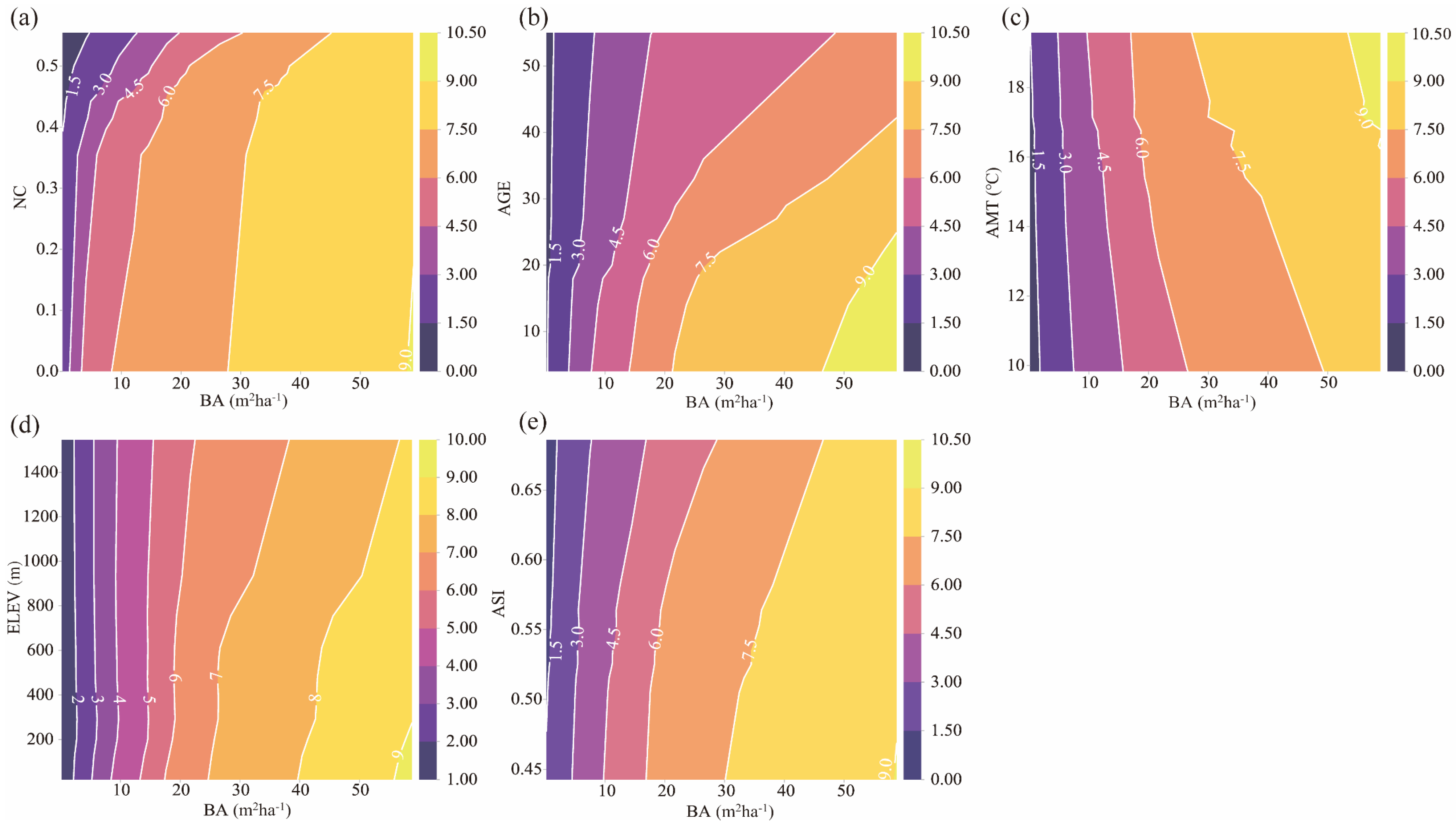
3.3.3. Two-Factor Interaction Analysis

The mean absolute SHAP values (Table S5) were calculated for the main (diagonal) and interactive effects (nondiagonal) of the influencing factors. Combinations of the top five nondiagonal SHAP values were selected. The interactive effects on stand productivity were analyzed using 2D PDP and were visualized intuitively. In Figure 4a, when BA was 0–20 m2ha−1, a low NC was more favorable for stand productivity in general than high NC at a certain BA. However, when BA > 20 m2ha−1, the response of stand productivity to the BA-NC interaction was not obvious. When the BA was <10 m2ha−1, the contribution of AGE to stand productivity was relatively weak (Figure 4b). However, the BA-AGE interaction on stand productivity was enhanced at BA > 15 m2ha−1. It is more favorable to promote stand productivity if it has a larger BA at a younger stand age. Figure 4c,d show that as BA increases and ELEV decreases, in addition to the simultaneous increase in BA and AMT, the more favorable the increase in stand productivity becomes. Figure 4e shows that when BA < 10 m2ha−1, the effect of ASI on stand productivity was not significant. When BA > 20 m2ha−1, a lower ASI was more favorable for stand productivity than a higher ASI.

4. Discussion

4.1. Tree Volume Model and Stand Productivity Parameter Selection

Tree stem volume is the basis for calculating stand productivity. In order to calculate the tree stem volume in the stand, we did not use destructive measurements, but used a Zhejiang one-way volume model, which carried out mass inventory measurements without felling trees. This one-way volume model has been applied in forest biomass assessment [48], forest resource monitoring [49], and stand growth calculation [50].
The Zhejiang one-way volume model was developed based on the general Chinese two-way volume model, i.e., V = a D b H c ( D is the caliper measurement-based DBH, and H is the tree height). Within Liu [36] work, the one-way volume model construction process is as follows: Firstly, the DBH in the Chinese two-way volume model is determined by calipers, while the current DBH is determined by d-tape (to avoid confusion, DBH in this study refers to d-tape measurement-based DBH unless otherwise stated). In order to solve the bias caused by the two tools for measuring DBH [51], an equation of caliper measurement-based DBH ( D ) and d-tape measurement-based DBH (D) was developed [52], i.e., D = a 1 + b 1 D (the meanings of a1 and b1 are shown in Equation (1)). Secondly, the tree height (H) was predicted by substituting the caliper measurement-based DBH into the height–diameter model. The height–diameter model is H = a 2 + b 2 / D + k (the meanings of a2, b2, and k are shown in Equation (1)). Finally, these two equations were combined with the two-way volume model to obtain Equation (1), which is similar to the construction process mentioned by Inoue et al. [53].
The parameters commonly used to calculate stand productivity are DBH [54], BA [8], biomass [55,56], volume [7,10], and net primary productivity [57]. But parameter selection is inconsistent across studies, probably because these parameters are highly correlated; e.g., DBH is the basis for the calculation of BA, volume, and biomass, and volume can be calculated biomass through conversion and expansion factors. However, whether stand productivity calculated from different parameters affects the robustness of the driving mechanism is unclear and can be refined in future studies. In this paper, we used the tree volume productivity in terms of periodic annual increment to express stand productivity. Our study only focuses on arbor trees, for which it is possible to calculate volume, but if the study includes bamboo or shrubs, we recommend using the biomass parameter.

4.2. Machine Learning Model and Influencing Factor Selection

The ML models, excepting XGBoost, performed more effectively than the LR model, indicating that the ML models can more comprehensively explain the nonlinear relationship between the influencing factors. Ensemble ML models generally performed better than individual ML models, although not exclusively (e.g., RF performed better than the voting model). Therefore, we compared the performance when selecting the model that best met the research objectives. The Autogluon model exhibited the optimal performance in this study. To the best of our knowledge, few studies have applied the Autogluon model to stand productivity forecasting; this model may be an important candidate for future research. We plotted the beeswarm plot of SHAP values of the other ML models (Figure S3). The distributions of SHAP values of independent variables are generally similar, and BA, NC, and AGE consistently rank in the top three in all models except the XGBoost model, indicating that the model selection is robust. The XGBoost model’s performance is the lowest, which may lead to biased SHAP values.
Dong et al. [30] noted that traditional statistical methods such as LR remain the most popular tools for identifying potential impacts. We found that BA, AGE, and ISOT had the same order and higher contribution rates, verifying the robustness of the global explanation based on the SHAP algorithm. The higher the SHAP value of an influencing factor, the more obvious it is to the model’s predicted outcome away from the baseline value [58], and the results of this characteristic can provide guidance to forest managers in implementing forest management.
In addition to ML model selection, determining the model’s independent variables is important. Climate, site conditions, and competition are the main drivers determining stand productivity [59]. In stand productivity studies, the choice of climate variables often varies, but AMT and AP are commonly chosen independent variables [7,8,10], and they are considered to be the main climatic factors influencing tree growth [60]. Our study refers to Liang et al. [7], where we not only considered AMT and AP, but also used ISOP, TS, and PWQ bioclimatic variables to characterize climatic conditions, which help explain the geographic distribution of natural populations affected by climate [61]. Stand conditions (e.g., soil fertility, slope and aspect, dominant height) determine the potential maximum growth of trees [60]. Considering that geographic conditions are widely used in stand productivity studies and to some extent reflect site conditions, we chose SLOP, ELEV, and ASPE. Competition mediates the effects of site and climate conditions on stand productivity [62]. In the productivity studies, commonly used indicators to represent competition are BA [7,56], the quadratic mean diameter [10], and the stand density index [60]. All these competition indicators are obtained based on DBH, so the selection of indicators may not be uniform. We also selected species diversity, stand structure diversity, and spatial distribution diversity. The effect of biodiversity on productivity is well known. Reasonable stand spatial structure promotes forest biomass accumulation, while the spatial distribution reflects tree development processes [63], so we chose NC and ASI, respectively. However, these two indicators are often used to analyze the mechanism of biomass influence [64,65], and less frequently used for stand productivity. We suggest that these two indicators be considered in future studies to provide a theoretical basis for optimizing spatial structure to enhance stand quality.

4.3. Basal Area Had Strongest Influence on Stand Productivity

The relationship between BA and stand productivity can be traced back nearly 100 years to the Wiedemann [66] study, which noted that stand density had no direct effect on volume growth between 20 and 35 m2ha−1 of basal area. A decade later, Langsaeter [67] presented curves describing forest volume growth versus standing volume, which had a wide elevated plateau in the middle. This is called Langsaeter’s hypothesis, in which volume growth follows a constant pattern over a broad range of standing volumes. Furthermore, Langsaeter [67] states that the limit of the constant pattern varies with site productivity and age. However, Assmann [68] argues that there must be an optimal basal area for each site, and that there is an optimal pattern between volume growth and basal area, i.e., that an increase in density above the optimal point would result in a reduction in growth. Moreover, more homogenously distributed BA or a stronger BA reduction risks natural regeneration of seedlings and affects productivity [69]. Recently, Allen and Burkhart [70], in their study of loblolly pine plantations, found that total volume growth increased with increasing stand density when accounting for site quality, age, and quadratic mean diameter, contradicting the constant and optimal patterns. Furthermore, in the studies of Gizachew and Brunner [71], Nilsson et al. [72], and del Río and Sterba [73], it was also found that there is a strong linear relationship between basal area and productivity. These studies have challenged traditional hypotheses. Allen and Burkhart [70] argue that two patterns are based on data from older mature forests, so the two growth–density relationships may not hold relative to young forests.
Consistent with previous studies [56,74], our study found that BA was the most important influencing factor. There was a positive correlation between BA and SHAP values; therefore, NBFs with a higher BA were more likely to have higher stand productivity, which is similar to the findings of some studies mentioned above, and also consistent with the results of Ali et al. [75], Ouyang et al. [6], Manuel Villa et al. [76], and Zhang et al. [27]. They concluded that forest communities with a larger BA usually have a larger leaf area index, which improves light interception efficiency and can produce more biomass through photosynthesis. Abundant biomass can lead to rapid growth in stand productivity [77,78]. Most previous studies have concluded that an increase in BA exacerbates tree competition and inhibits an increase in stand productivity [8,10]. Our findings may seem contrary to these, but we believe that the most important metric was to recognize the expression of stand productivity in the study. More specifically, the increment and incremental rate constitute two different concepts [79]. Our study showed that the mean annual increment increased in parallel with BA, but the mean annual incremental rate unsurprisingly decreased (Figure S4a).
We found that the smaller the BA, the greater its negative contribution to the predicted results for stand productivity. This result occurred because stands with a small BA tended to be saplings and young trees, which may grow slowly owing to low light energy utilization and increased water competition [80]. Moreover, this stage is more susceptible to negative density dependence, which leads to pests and diseases that kill trees and reduce stand productivity [81]. Previous scholars analyzed the negative density dependence at the different growth stages of saplings (mean DBH < 5 cm), young trees (5 cm ≤ mean DBH < 10 cm), and large trees (mean DBH ≥ 10 cm) in NBFs in Zhejiang Province, and concluded that the negative density dependence was reduced only after the small tree stage [82,83]. This result may explain why the SHAP values for BA were mostly negative for saplings and young trees in the present study, whereas the SHAP values for large trees were mostly positive (Figure S4b). In addition, our view is consistent with those of Yuan et al. [84] and Stephenson et al. [85], in that a higher BA implies more trees with a large DBH in the plots, and that these large trees may contribute more to the increase in productivity. Ma et al. (2021) argued that the biomass allocation strategy during forest growth is also an important factor influencing stand productivity. With increasing age, the proportion of biomass allocated to the stem is higher than that allocated to the roots [86,87].

4.4. Stand Spatial Structure: The Main Influencer of Stand Productivity

In this study, NC was negatively correlated with SHAP values, and the SHAP values changed from positive to negative when NC exceeded 0.44, which is consistent with recent studies suggesting a negative effect [88,89]. This result may be explained by an increasing NC causing competitive pressures between trees to inhibit growth, leading to a weakening of mean annual DBH growth, which in turn has a dampening effect on stand productivity. We also found (Figure 4a) that at the BA < 20 m2ha−1 stage, when BA was certain, stand productivity at a smaller NC was higher than that at a larger NC. However, this effect was weakened when BA was > 20 m2ha−1. This result may have occurred because a lower stand structural heterogeneity promotes stand growth [90]. In contrast, at the stage of high size inequality, trees with a larger DBH received higher absorbed photosynthetically active radiation and light-use efficiency, which increased the growth rate; however, smaller trees were inhibited by neighboring trees, which had a greater impact on the decrease in stand growth [91].
The distribution of trees in stands can be heterogeneous. Clustered or fragmented distribution patterns influence the growth of individual trees [23]. The SHAP value gradually increased from aggregated distribution (0.5 < ASI ≤ 1) to random distribution (0.25 < ASI ≤ 0.5) to uniform distribution (0 < ASI ≤ 0.25). When the ASI was less than 0.55 and gradually decreased, the SHAP value was positive and continued to increase. This indicates that the more uniform the spatial distribution of trees, the more conducive the distribution was in improving stand productivity. During the succession of broadleaf evergreen forests in the subtropics, the distribution pattern generally shows a trend from an aggregated distribution to a random distribution owing to mechanisms such as density constraints and diffusion limitations [92]. During this process, small trees can fill gaps that occur over time and may utilize unused space and light to increase the overall stand productivity [93]. Another explanation for this dynamic (Vanhellemont et al. [94]) is that single trees in advantageous spatial locations will remain in the stand and suppress weaker and less efficient neighboring trees. Wang et al. [89] also noted in a study on the mean annual DBH growth of NBF that the stand spatial structure was gradually optimized by self-thinning, and that DBH growth under aggregated distribution was obviously lower than that under uniform distribution.
The SHAP values of NC and ASI have thresholds, and values greater than the threshold will make the SHAP value negative; this principle indicates the importance of rationally regulating the stand spatial structure to promote tree growth, because the stand spatial structure may be related to the accumulation of forest biomass [64,95]. We portrayed the direct mechanisms by which stand spatial structure affected stand productivity, but have not yet considered its mediating effects. In future studies, it will be possible to explore the variables that are mediated by stand spatial structure, which may help clarify the integrated influence mechanism of stand spatial structure on stand productivity.

4.5. Increasing Stand Productivity Through Effective Forest Management

Our study found that BA, NC, AGE, and ASI reflected forest stand characteristics, indicating the importance of improving stand productivity through targeted forest management. Therefore, to improve NBF stand productivity, goal trees in low-BA stands were managed, and measures such as thinning, cutting, and singling were used to optimize stand spatial structure, reduce clustering distribution, and maintain a reasonable DBH neighborhood comparison. An artificially promoted natural regeneration approach was previously adopted in high-BA stands to establish unevenly aged stratified mixed stands and promote regeneration by adjusting the positioning, nutrient content, and angle of leaves within the canopies [96]. The relationship between NC and SHAP values, as pointed out by Zeller and Pretzsch [93], indicates that structural diversity does not always have a positive effect on stand productivity, and increased stand productivity may not occur at all growth stages. This suggests a focus on full-cycle, differentiated forest management, and adjusting the stand density and tree species composition through thinning and replanting. Because stand productivity generally declines with increasing stand age, the age at which maximum stand productivity occurs is an important basis for forest managers to determine the optimal felling cycle [97]. Although most of the NBFs in Zhejiang Province are young forests, they are also expected to become middle-aged or mature forests in 20 years. The forestry department should formulate forest regeneration policies, thin mature forests appropriately, and cultivate reserve resources in these plots through the artificially promoted natural regeneration approach and replanting. In addition, low elevation is more conducive to promoting stand productivity at a certain BA (Figure 4d). Meanwhile, the importance of ISOT and AMT ranked in the top five and was positively correlated with SHAP values (Figure 4a). Therefore, forest management zoning should be carried out in relation to topography and climate, and site-specific forest management policies should be developed. Finally, the positive correlation between higher SIMP and SHAP illustrates the importance of planting native tree species and avoiding pure forest plantations, and emphasizes the need to promote biological conservation in forest management practices.

5. Conclusions

Understanding the drivers of stand productivity is essential for NBF management in the context of “carbon peak, neutrality”. This study used 642 CFI plots in Zhejiang Province in 2014 and 2019, constructed an interpretable ML framework based on the SHAP algorithm and PDP, and analyzed the global and local explanations and major interactions of drivers (species diversity, structure diversity, spatial distribution diversity, stand density, stand age, geographical condition, and meteorological condition) on the stand productivity of NBFs. We found the following. (1) The Autogluon model exhibited the optimal forecasting performance. (2) The global explanation indicated that BA, NC, and AGE were the main influencing factors of stand productivity. (3) Local interpretation found that increasing BA, as well as controlling NC and ASI below 0.45 and 0.55, respectively, helped to increase stand productivity. Stand age was negatively correlated with stand productivity, emphasizing the importance of slowing aging through scientific forest management. Topographic factors emphasize the importance of advantageous site conditions, with gentle slopes and low elevations contributing most to improving stand productivity. (4) BA showed the strongest interactions with NC, AGE, ELEV, AMT, and ASI. Collectively, SHAP values helped evaluate the effects of stand and environmental factors on the stand productivity of NBFs and emphasize forest management by designing differentiated strategies. Furthermore, this study also enhances our understanding of the importance of BA, NC, and AGE in NBF management, and can provide a theoretical basis for forestry managers to conduct forest management according to local conditions and optimize the layout areas and direction of NBF management.

Supplementary Materials

The following supporting information can be downloaded at https://www.mdpi.com/article/10.3390/f16010095/s1, Figure S1. Driver Z-score based on Boruta’s algorithm; Figure S2. The prediction results of machine learning models; Figure S3. Beeswarm plot of SHAP values of other machine learning models; Figure S4. (a) Scatter plot of BA and stand growth rate, (b) Distribution of SHAP values for BA in saplings, young trees, and large trees. Table S1. Parameters of one-variable tree volume model; Table S2. Hyperparameter optimization range; Table S3. Results of hyperparameter optimization; Table S4. Results of VIF test; Table S5. Pairwise SHAP interaction values (nondiagonal) of the drivers; Table S6. Results of multiple linear regression [98,99,100,101,102,103,104,105].

Author Contributions

Q.D.: writing—original draft and methodology. C.Z.: writing—review and editing, visualization, and project administration. B.J.: software and funding acquisition. S.X.: validation and data collection. B.X.: data collection and software. J.W.: data collection. Z.W.: formal analysis. All authors have read and agreed to the published version of the manuscript.

Funding

This research was funded by the Annual monitoring of forest ecological status in Zhejiang Province (245002) and “Pioneer” and “Leading Goose” R&D Program of Zhejiang (2022C02053).

Data Availability Statement

The raw data supporting the conclusions of this article will be made available by the authors on request.

Conflicts of Interest

Sen Xu is employed by Zhejiang Forestry Survey planning and design Co., Ltd.; his employer’s company was not involved in this study, and there is no relation between this research and their company. The remaining authors declare that the research was conducted in the absence of any commercial or financial relationships that could be construed as potential conflicts of interest. The funders had no role in the design of the study; in the collection, analyses, or interpretation of data; in the writing of the manuscript; or in the decision to publish the results.

References

  1. Souza, C.R.; Mariano, R.F.; Maia, V.A.; Pompeu, P.V.; Santos, R.M.D.; Fontes, M.A.L. Carbon stock and uptake in the high-elevation tropical montane forests of the threatened Atlantic Forest hotspot: Ecosystem function and effects of elevation variation. Sci. Total Environ. 2023, 882, 163503. [Google Scholar] [CrossRef]
  2. Crow, T.R.; Dey, D.C.; Riemenschneider, D. Forest Productivity: Producing Goods and Services for People; U.S. Department of Agriculture, Forest Service, North Central Research Station: Madison, WI, USA, 2006. [Google Scholar]
  3. Mamo, N.; Sterba, H. Site index functions for Cupressus lusitanica at Munesa Shashemene, Ethiopia. For. Ecol. Manag. 2006, 237, 429–435. [Google Scholar] [CrossRef]
  4. Herraiz, A.D.; Salazar-Zarzosa, P.C.; Mesas, F.J.; Arenas-Castro, S.; Ruiz-Benito, P.; Villar, R. Modelling aboveground biomass and productivity and the impact of climate change in Mediterranean forests of South Spain. Agric. For. Meteorol. 2023, 337, 109498. [Google Scholar] [CrossRef]
  5. Sotomayor, L.N.; Cracknell, M.J.; Musk, R. Supervised machine learning for predicting and interpreting dynamic drivers of plantation forest productivity in northern Tasmania, Australia. Comput. Electron. Agric. 2023, 209, 107804. [Google Scholar] [CrossRef]
  6. Ouyang, S.; Xiang, W.; Wang, X.; Xiao, W.; Chen, L.; Li, S.; Sun, H.; Deng, X.; Forrester, D.I.; Zeng, L.; et al. Effects of stand age, richness and density on productivity in subtropical forests in China. J. Ecol. 2019, 107, 2266–2277. [Google Scholar] [CrossRef]
  7. Liang, J.; Crowther, T.W.; Picard, N.; Wiser, S.; Zhou, M.; Alberti, G.; Schulze, E.-D.; McGuire, A.D.; Bozzato, F. Positive biodiversity-productivity relationship predominant in global forests. Science 2016, 354, 196. [Google Scholar] [CrossRef]
  8. Kweon, D.; Comeau, P.G. Factors influencing productivity of pine-dominated stands in South Korea. J. Environ. Manag. 2023, 330, 117250. [Google Scholar] [CrossRef] [PubMed]
  9. Salazar Zarzosa, P.; Diaz Herraiz, A.; Olmo, M.; Ruiz-Benito, P.; Barron, V.; Bastias, C.C.; de la Riva, E.G.; Villar, R. Linking functional traits with tree growth and forest productivity in Quercus ilex forests along a climatic gradient. Sci. Total Environ. 2021, 786, 147468. [Google Scholar] [CrossRef]
  10. Wang, Z.; Zhang, X.; Chhin, S.; Zhang, J.; Duan, A. Disentangling the effects of stand and climatic variables on forest productivity of Chinese fir plantations in subtropical China using a random forest algorithm. Agric. For. Meteorol. 2021, 304, 108412. [Google Scholar] [CrossRef]
  11. Yang, L.; Zhang, J.; Wang, J.; Gu, Y.; Han, S. A linear positive relationship between tree species diversity and forest productivity across forest-dominated natural reserves on a large spatial scale. For. Ecol. Manag. 2023, 548, 121409. [Google Scholar] [CrossRef]
  12. Kara, F.; Keleş, S.Ö. Tree species richness influence productivity and anatomical characteristics in mixed fir-pine-beech forests. Plant Ecol. 2023, 224, 479–489. [Google Scholar] [CrossRef]
  13. Chetelat, R.T.; Pertuzé, R.A.; Faúndez, L.; Graham, E.B.; Jones, C.M. Distribution, ecology and reproductive biology of wild tomatoes and related nightshades from the Atacama Desert region of northern Chile. Euphytica 2008, 167, 77–93. [Google Scholar] [CrossRef]
  14. Rosas, T.; Mencuccini, M.; Barba, J.; Cochard, H.; Saura-Mas, S.; Martinez-Vilalta, J. Adjustments and coordination of hydraulic, leaf and stem traits along a water availability gradient. New Phytol. 2019, 223, 632–646. [Google Scholar] [CrossRef]
  15. Oboite, F.O.; Comeau, P.G. Competition and climate influence growth of black spruce in western boreal forests. For. Ecol. Manag. 2019, 443, 84–94. [Google Scholar] [CrossRef]
  16. Marcatti, G.E.; Resende, R.T.; Resende, M.D.V.; Ribeiro, C.A.A.S.; dos Santos, A.R.; da Cruz, J.P.; Leite, H.G. GIS-based approach applied to optimizing recommendations of Eucalyptus genotypes. For. Ecol. Manag. 2017, 392, 144–153. [Google Scholar] [CrossRef]
  17. Ameray, A.; Cavard, X.; Bergeron, Y. Climate change may increase Quebec boreal forest productivity in high latitudes by shifting its current composition. Front. For. Glob. Chang. 2023, 6, 1020305. [Google Scholar] [CrossRef]
  18. Ammer, C. Diversity and forest productivity in a changing climate. New Phytol. 2019, 221, 50–66. [Google Scholar] [CrossRef]
  19. Baach, E.; Himes, A.; Polinko, A.; Granger, J.J.; Zhou, Q. Diversity-productivity relationships in forests of the southeastern United States: Leveraging national inventory data and tree functional traits. For. Ecol. Manag. 2022, 521, 120426. [Google Scholar] [CrossRef]
  20. Kohyama, T.I.; Sheil, D.; Sun, I.F.; Niiyama, K.; Suzuki, E.; Hiura, T.; Nishimura, N.; Hoshizaki, K.; Wu, S.H.; Chao, W.C.; et al. Contribution of tree community structure to forest productivity across a thermal gradient in eastern Asia. Nat. Commun. 2023, 14, 1113. [Google Scholar] [CrossRef]
  21. Ma, S.; Wang, X.; Miao, W.; Wang, X.; Sun, H.; Guo, Z. Relative influence of environmental, stand factors and functional traits on allocation of forest productivity during the restoration of subtropical forests in central China. For. Ecol. Manag. 2021, 482, 118814. [Google Scholar] [CrossRef]
  22. Forrester, D.I.; Bauhus, J. A Review of Processes Behind Diversity—Productivity Relationships in Forests. Curr. For. Rep. 2016, 2, 45–61. [Google Scholar] [CrossRef]
  23. Forrester, D.I. Linking forest growth with stand structure: Tree size inequality, tree growth or resource partitioning and the asymmetry of competition. For. Ecol. Manag. 2019, 447, 139–157. [Google Scholar] [CrossRef]
  24. Forrester, D.I.; Kohnle, U.; Albrecht, A.T.; Bauhus, J. Complementarity in mixed-species stands of Abies alba and Picea abies varies with climate, site quality and stand density. For. Ecol. Manag. 2013, 304, 233–242. [Google Scholar] [CrossRef]
  25. Garber, S.M.; Maguire, D.A. Stand Productivity and Development in Two Mixed-Species Spacing Trials in the Central Oregon Cascades. For. Sci. 2004, 50, 92–105. [Google Scholar] [CrossRef]
  26. John, R.; Chen, J.; Kim, Y.; Ou-yang, Z.-t.; Xiao, J.; Park, H.; Shao, C.; Zhang, Y.; Amarjargal, A.; Batkhshig, O.; et al. Differentiating anthropogenic modification and precipitation-driven change on vegetation productivity on the Mongolian Plateau. Landsc. Ecol. 2015, 31, 547–566. [Google Scholar] [CrossRef]
  27. Zhang, M.; Fan, X.; Yue, Q.; Han, Z.; Huang, Y. Effects of Biotic and Abiotic Factors on Productivity of Coniferous and Broad-Leaved Mixed Forest in Jiaohe, Jilin Province. Sci. Silvae Sin. 2023, 59, 71–77. [Google Scholar]
  28. Zou, J.; Luo, Y.; Seidl, R.; Thom, D.; Liu, J.; Geres, L.; Richter, T.; Ye, L.; Zheng, W.; Ma, L.; et al. No generality in biodiversity-productivity relationships along elevation in temperate and subtropical forest landscapes. For. Ecosyst. 2024, 11, 100187. [Google Scholar] [CrossRef]
  29. Rocha, S.J.S.S.d.; Torres, C.M.M.E.; Villanova, P.H.; Tavares Júnior, I.d.S.; Rufino, M.P.M.X.; Romero, F.M.B.; Jacovine, L.A.G.; de Morais Junior, V.T.M.; França, L.C.d.J.; Schettini, B.L.S.; et al. Machine learning methods: Modeling net growth in the Atlantic Forest of Brazil. Ecol. Inform. 2024, 81, 102564. [Google Scholar] [CrossRef]
  30. Dong, L.; Lin, X.; Bettinger, P.; Liu, Z. The contributions of stand characteristics on carbon sequestration potential are triple that of climate variables for Larix spp. plantations in northeast China. Sci. Total Environ. 2024, 911, 168726. [Google Scholar] [CrossRef]
  31. Becknell, J.M.; Powers, J.S. Stand age and soils as drivers of plant functional traits and aboveground biomass in secondary tropical dry forest. Can. J. For. Res. 2014, 44, 604–613. [Google Scholar] [CrossRef]
  32. Qiao, X.; Hautier, Y.; Geng, Y.; Wang, S.; Wang, J.; Zhang, N.; Zhang, Z.; Zhang, C.; Zhao, X.; von Gadow, K. Biodiversity contributes to stabilizing ecosystem productivity across spatial scales as much as environmental heterogeneity in a large temperate forest region. For. Ecol. Manag. 2023, 529, 120695. [Google Scholar] [CrossRef]
  33. Hu, J.; Xu, J.; Li, M.; Jiang, Z.; Mao, J.; Feng, L.; Miao, K.; Li, H.; Chen, J.; Bai, Z.; et al. Identification and validation of an explainable prediction model of acute kidney injury with prognostic implications in critically ill children: A prospective multicenter cohort study. EClinicalMedicine 2024, 68, 102409. [Google Scholar] [CrossRef]
  34. Ma, Z.; Wang, R.; Song, G.; Zhang, K.; Zhao, Z.; Wang, J. Interpretable ensemble prediction for anaerobic digestion performance of hydrothermal carbonization wastewater. Sci. Total Environ. 2024, 908, 168279. [Google Scholar] [CrossRef]
  35. Museru, M.L.; Nazari, R.; Giglou, A.N.; Opare, K.; Karimi, M. Advancing flood damage modeling for coastal Alabama residential properties: A multivariable machine learning approach. Sci. Total Environ. 2024, 907, 167872. [Google Scholar] [CrossRef]
  36. Liu, A. Mathematical modeling of volume of living tree in Zhejiang Province. J. Zhejiang For. Sci. Technol. 1986, 4, 25–30. [Google Scholar]
  37. Hui, G.; Gadow, K.v.; Albert, M. A new parameter for stand spatial structure neighbourhood comparison. For. Res. 1999, 12, 1–6. [Google Scholar]
  38. Fick, S.E.; Hijmans, R.J. WorldClim 2: New 1-km spatial resolution climate surfaces for global land areas. Int. J. Climatol. 2017, 37, 4302–4315. [Google Scholar] [CrossRef]
  39. Erickson, N.; Mueller, J.; Shirkov, A.; Zhang, H.; Larroy, P.; Li, M.; Smola, A. AutoGluon-Tabular: Robust and Accurate AutoML for Structured Data. arXiv 2020, arXiv:2003.06505. [Google Scholar]
  40. Qi, W.; Xu, C.; Xu, X. AutoGluon: A revolutionary framework for landslide hazard analysis. Nat. Hazards Res. 2021, 1, 103–108. [Google Scholar] [CrossRef]
  41. Zhang, Y.; Zhao, Y.; Feng, Y.; Yu, Y.; Li, Y.; Li, J.; Ren, Z.; Chen, S.; Feng, L.; Pan, J.; et al. Novel Intelligent System Based on Automated Machine Learning for Multiobjective Prediction and Early Warning Guidance of Biogas Performance in Industrial-Scale Garage Dry Fermentation. ACS EST Eng. 2023, 4, 139–152. [Google Scholar] [CrossRef]
  42. Lin, X.; Hou, J.; Wu, X.; Lin, D. Elucidating the impacts of microplastics on soil greenhouse gas emissions through automatic machine learning frameworks. Sci. Total Environ. 2024, 916, 170308. [Google Scholar] [CrossRef]
  43. Lai, J.; Zou, Y.; Zhang, S.; Zhang, X.; Mao, L.; Zhang, W.H. glmm.hp: An R package for computing individual effect of predictors in generalized linear mixed models. J. Plant Ecol. 2022, 15, 1302–1307. [Google Scholar] [CrossRef]
  44. Li, Z. Extracting spatial effects from machine learning model using local interpretation method: An example of SHAP and XGBoost. Comput. Environ. Urban Syst. 2022, 96, 101845. [Google Scholar] [CrossRef]
  45. Shapley, L.S. A Value for n-Person Games; Princeton University Press: Princeton, NJ, USA, 1953. [Google Scholar]
  46. Xu, Y.; Zhang, D.; Lin, J.; Peng, Q.; Lei, X.; Jin, T.; Wang, J.; Yuan, R. Prediction of phytoplankton biomass and identification of key influencing factors using interpretable machine learning models. Ecol. Indic. 2024, 158, 111320. [Google Scholar] [CrossRef]
  47. Lundberg, S.M.; Lee, S.-I. A unified approach to interpreting model predictions. Neural Inf. Process. Syst. 2017, 30, 4768–4777. [Google Scholar]
  48. Ji, B.; Tao, J.; Zhang, G.; Du, Q.; Yao, H.; Xu, J. Zhejiang Province’s forest vegetation biomass assessment for guaranteed accuracy. J. Zhejiang AF Univ. 2012, 29, 328–334. [Google Scholar]
  49. Ji, B.; Zhang, G.; Zhao, G.; Lai, J. A Technical Method of Dynamic Forest Resources Monitoring at the County Level Based on the Permanent Plots. For. Resour. Manag. 2009, 5, 50–53. [Google Scholar]
  50. Sun, K.; Wu, D.; Sun, H. Effects of Mixed Betula luminifera and Phyllostachys edulis with Different Proportions on the Growth of Cunninghamia lanceolata after Thinning. For. Grassl. Resour. Res. 2024, 2, 124–132. [Google Scholar]
  51. Brickell, J.E. More on Diameter Tape and Calipers. J. For. 1970, 68, 169–170. [Google Scholar]
  52. Mao, Z. Compilation of the two-way volume model for Zhejiang Province. J. Zhejiang AF Univ. 1988, 5, 75–80. [Google Scholar]
  53. Inoue, A.; Sakamoto, S.; Suga, H.; Kitazato, H.; Sakuta, K. Construction of one-way volume table for the three major useful bamboos in Japan. J. For. Res. 2013, 18, 323–334. [Google Scholar] [CrossRef]
  54. Zhang, Z.; Zhou, L.; Lu, C.; Fu, Y.; Gu, Z.; Chen, Y.; Zhang, G.; Zhou, X. Drought- induced decrease in tree productivity mainly mediated by the maximum growth rate and growing-season length in a subtropical forest. For. Ecol. Manag. 2024, 563, 121985. [Google Scholar] [CrossRef]
  55. Hisano, M.; Ghazoul, J.; Chen, X.; Chen, H.Y.H. Functional diversity enhances dryland forest productivity under long-term climate change. Sci. Adv. 2024, 10, eadn4152. [Google Scholar] [CrossRef]
  56. Paquette, A.; Messier, C. The effect of biodiversity on tree productivity: From temperate to boreal forests. Glob. Ecol. Biogeogr. 2010, 20, 170–180. [Google Scholar] [CrossRef]
  57. Zhang, X.; Su, J.; Ji, Y.; Zhao, J.; Gao, J. Nitrogen deposition affects the productivity of planted and natural forests by modulating forest climate and community functional traits. For. Ecol. Manag. 2024, 563, 121970. [Google Scholar] [CrossRef]
  58. Jain, S.; Jain, S.; Wolf, I.T.; Lee, J.; Tong, Y.W. A comprehensive review on operating parameters and different pretreatment methodologies for anaerobic digestion of municipal solid waste. Renew. Sustain. Energy Rev. 2015, 52, 142–154. [Google Scholar] [CrossRef]
  59. Madrigal-González, J.; Zavala, M.A. Competition and tree age modulated last century pine growth responses to high frequency of dry years in a water limited forest ecosystem. Agric. For. Meteorol. 2014, 192, 18–26. [Google Scholar] [CrossRef]
  60. Calama, R.; Conde, M.; de-Dios-García, J.; Madrigal, G.; Vázquez-Piqué, J.; Gordo, F.J.; Pardos, M. Linking climate, annual growth and competition in a Mediterranean forest: Pinus pinea in the Spanish Northern Plateau. Agric. For. Meteorol. 2019, 264, 309–321. [Google Scholar] [CrossRef]
  61. Beyer, R.M.; Krapp, M.; Manica, A. High-resolution terrestrial climate, bioclimate and vegetation for the last 120,000 years. Sci. Data 2020, 7, 236. [Google Scholar] [CrossRef]
  62. Wang, Y.; Pederson, N.; Ellison, A.M.; Buckley, H.L.; Case, B.S.; Liang, E.; Julio Camarero, J. Increased stem density and competition may diminish the positive effects of warming at alpine treeline. Ecology 2016, 97, 1668–1679. [Google Scholar] [CrossRef]
  63. Pretzsch, H. Analysis and modeling of spatial stand structures. Methodological considerations based on mixed beech-larch stands in Lower Saxony. For. Ecol. Manag. 1997, 97, 237–253. [Google Scholar] [CrossRef]
  64. Huang, X.; Chen, Y.; Tan, H.; Zhang, Y.; Yu, S.; Chen, X.; Yu, K.; Liu, J. Extraction of the spatial structure of Chinese fir plantations stands based on unmanned aerial vehicle and its effect on AGB. For. Ecol. Manag. 2024, 558, 121800. [Google Scholar] [CrossRef]
  65. Yang, B.; Ma, R.; Zhai, J.; Du, J.; Bai, J.; Zhang, W. Stand spatial structure is more important than species diversity in enhancing the carbon sink of fragile natural secondary forest. Ecol. Indic. 2024, 558, 121800. [Google Scholar] [CrossRef]
  66. Wiedemann, E. Die Rotbuche 1931. Fortführung des Berichtes von Geheimrat Schwappach 1911 über die Preussischen BuchenVersuchsfläche; Schaper: Niedersachsen, Germany, 1932. [Google Scholar]
  67. Langsaeter, A. Om tynning i enaldret gran-og furuskog (About thinning in even-aged stands of spruce). Nor. Skogforsokresen 1941, 8, 131–216. [Google Scholar]
  68. Assmann, E. Grundflächen- und Volumzuwachs der Rotbuche bei verschiedenen Durchforstungsgraden. Forstwiss. Cent. 1950, 69, 256–286. [Google Scholar] [CrossRef]
  69. Pretzsch, H.; Biber, P.; Uhl, E.; Dauber, E. Long-term stand dynamics of managed spruce–fir–beech mountain forests in Central Europe: Structure, productivity and regeneration success. Forestry 2015, 88, 407–428. [Google Scholar] [CrossRef]
  70. Allen, M.G.; Burkhart, H.E. Growth-Density Relationships in Loblolly Pine Plantations. For. Sci. 2019, 65, 250–264. [Google Scholar] [CrossRef]
  71. Gizachew, B.; Brunner, A. Density–growth relationships in thinned and unthinned Norway spruce and Scots pine stands in Norway. Scand. J. For. Res. 2011, 26, 543–554. [Google Scholar] [CrossRef]
  72. Nilsson, U.; Agestam, E.; Ekö, P.-M.; Elfving, B.; Fahlvik, N.; Johansson, U.; Karlsson, K.; Lundmark, T.; Wallentin, C. Thinning of Scots pine and Norway spruce monocultures in Sweden: Effects of different thinning programmes on stand level gross- and net stem volume production. Stud. For. Suec. 2010, 219, 1–46. [Google Scholar]
  73. del Río, M.; Sterba, H. Comparing volume growth in pure and mixed stands of Pinus sylvestris and Quercus pyrenaica. Ann. For. Sci. 2009, 66, 502. [Google Scholar] [CrossRef]
  74. Lohbeck, M.; Poorter, L.; Martinez-Ramos, M.; Bongers, F. Biomass is the main driver of changes in ecosystem process rates during tropical forest succession. Ecology 2015, 96, 1242–1252. [Google Scholar] [CrossRef]
  75. Ali, A.; Lin, S.L.; He, J.K.; Kong, F.M.; Yu, J.H.; Jiang, H.S. Big-sized trees overrule remaining trees’ attributes and species richness as determinants of aboveground biomass in tropical forests. Glob. Chang. Biol. 2019, 25, 2810–2824. [Google Scholar] [CrossRef] [PubMed]
  76. Manuel Villa, P.; Ali, A.; Venâncio Martins, S.; Nolasco de Oliveira Neto, S.; Cristina Rodrigues, A.; Teshome, M.; Alvim Carvalho, F.; Heringer, G.; Gastauer, M. Stand structural attributes and functional trait composition overrule the effects of functional divergence on aboveground biomass during Amazon forest succession. For. Ecol. Manag. 2020, 477, 118481. [Google Scholar] [CrossRef]
  77. Miao, W.; Ma, S.; Guo, Z.; Sun, H.; Wang, X.; Lyu, Y.; Wang, X.; Ma, K. Effects of biodiversity, stand factors and functional identity on biomass and productivity during the restoration of subtropical forests in Central China. J. Plant Ecol. 2022, 15, 385–398. [Google Scholar] [CrossRef]
  78. Xu, K.; Wang, X.; Liang, P.; Wu, Y.; An, H.; Sun, H.; Wu, P.; Wu, X.; Li, Q.; Guo, X.; et al. A new tree-ring sampling method to estimate forest productivity and its temporal variation accurately in natural forests. For. Ecol. Manag. 2019, 433, 217–227. [Google Scholar] [CrossRef]
  79. Yuan, Z.; Ali, A.; Wang, S.; Gazol, A.; Freckleton, R.; Wang, X.; Lin, F.; Ye, J.; Zhou, L.; Hao, Z.; et al. Abiotic and biotic determinants of coarse woody productivity in temperate mixed forests. Sci. Total Environ. 2018, 630, 422–431. [Google Scholar] [CrossRef]
  80. van der Sande, M.T.; Peña-Claros, M.; Ascarrunz, N.; Arets, E.J.M.M.; Licona, J.C.; Toledo, M.; Poorter, L.; Hector, A. Abiotic and biotic drivers of biomass change in a Neotropical Forest. J. Ecol. 2017, 105, 1223–1234. [Google Scholar] [CrossRef]
  81. Yang, Q.; Ding, J.; Siemann, E.; Godoy, O. Biogeographic variation of distance-dependent effects in an invasive tree species. Funct. Ecol. 2019, 33, 1135–1143. [Google Scholar] [CrossRef]
  82. Wu, C.; Yuan, W.; Sheng, W.; Huan, Y.; Chen, Q.; Shen, A.; Zhu, J.; Jiang, B. Spatial distribution patterns and associations of tree species in typical natural secondary forest communities in Zhejiang Province. Acta Ecol. Sin. 2018, 38, 537–549. [Google Scholar]
  83. Zhong, L.; Liu, J.; Ding, W.; Tian, Y.; Chen, J.; Li, M.; Yu, M. Comparative research of the structures of plant functional groups in different successional stages of lowland secondary forests in Zhejiang Province. J. Zhejiang Univ. (Sci. Ed.) 2014, 41, 593–599. [Google Scholar]
  84. Yuan, Z.; Ali, A.; Sanaei, A.; Ruiz-Benito, P.; Jucker, T.; Fang, L.; Bai, E.; Ye, J.; Lin, F.; Fang, S.; et al. Few large trees, rather than plant diversity and composition, drive the above-ground biomass stock and dynamics of temperate forests in northeast China. For. Ecol. Manag. 2021, 481, 118698. [Google Scholar] [CrossRef]
  85. Stephenson, N.L.; Das, A.J.; Condit, R.; Russo, S.E.; Baker, P.J.; Beckman, N.G.; Coomes, D.A.; Lines, E.R.; Morris, W.K.; Ruger, N.; et al. Rate of tree carbon accumulation increases continuously with tree size. Nature 2014, 507, 90–93. [Google Scholar] [CrossRef]
  86. Luo, Y.; Wang, X.; Zhang, X.; Booth, T.H.; Lu, F. Root:shoot ratios across China’s forests: Forest type and climatic effects. For. Ecol. Manag. 2012, 269, 19–25. [Google Scholar] [CrossRef]
  87. Mokany, K.; Raison, R.J.; Prokushkin, A.S. Critical analysis of root: Shoot ratios in terrestrial biomes. Glob. Chang. 2005, 12, 84–96. [Google Scholar] [CrossRef]
  88. Sun, H.; Diao, S.; Liu, R.; Forrester, D.; Soares, A.; Saito, D.; Dong, R.; Jiang, J. Relationship between size inequality and stand productivity is modified by self-thinning, age, site and planting density in Sassafras tzumu plantations in central China. For. Ecol. Manag. 2018, 422, 199–206. [Google Scholar] [CrossRef]
  89. Wang, J.; Xu, S.; Ji, B.; Du, Q. Effects of topography and stand spatial structure on the diameter at breast height growth of major pioneer tree species of natural broad-leaved mixed forests in Zhejiang Province, China. Chin. J. Appl. Ecol. 2024, 35, 298–306. [Google Scholar]
  90. Soares, A.A.V.; Leite, H.G.; Souza, A.L.; Silva, S.R.; Lourenço, H.M.; Forrester, D.I. Increasing stand structural heterogeneity reduces productivity in Brazilian Eucalyptus monoclonal stands. For. Ecol. Manag. 2016, 373, 26–32. [Google Scholar] [CrossRef]
  91. Luu, T.C.; Binkley, D.; Stape, J.L. Neighborhood uniformity increases growth of individual Eucalyptus trees. For. Ecol. Manag. 2013, 289, 90–97. [Google Scholar] [CrossRef]
  92. Zhu, Y.; Mi, X.; Ren, H.; Ma, K. Density dependence is prevalent in a heterogeneous subtropical forest. Oikos 2010, 119, 109–119. [Google Scholar] [CrossRef]
  93. Zeller, L.; Pretzsch, H. Effect of forest structure on stand productivity in Central European forests depends on developmental stage and tree species diversity. For. Ecol. Manag. 2019, 434, 193–204. [Google Scholar] [CrossRef]
  94. Vanhellemont, M.; Bijlsma, R.-J.; De Keersmaeker, L.; Vandekerkhove, K.; Verheyen, K. Species and structural diversity affect growth of oak, but not pine, in uneven-aged mature forests. Basic Appl. Ecol. 2018, 27, 41–50. [Google Scholar] [CrossRef]
  95. Liu, L.; Zeng, F.; Song, T.; Wang, K.; Du, H. Stand Structure and Abiotic Factors Modulate Karst Forest Biomass in Southwest China. Forests 2020, 11, 443. [Google Scholar] [CrossRef]
  96. Coomes, D.A.; Holdaway, R.J.; Kobe, R.K.; Lines, E.R.; Allen, R.B. A general integrative framework for modelling woody biomass production and carbon sequestration rates in forests. J. Ecol. 2011, 100, 42–64. [Google Scholar] [CrossRef]
  97. Curtis, R.O. Technical Commentary: A New Look at an Old Question—Douglas-Fir Culmination Age. West. J. Appl. For. 1992, 7, 97–99. [Google Scholar] [CrossRef]
  98. Breiman, L. Random forests. Mach. Learn. 2001, 45, 5–32. [Google Scholar] [CrossRef]
  99. Chai, Z. An R Package for Forest Spatial Structure Analysis. 2016. Available online: https://github.com/Zongzheng/forestSAS (accessed on 18 February 2024).
  100. Chen, T.; Guestrin, C. XGBoost: A Scalable Tree Boosting System. In Proceedings of the 22nd ACM SIGKDD International Conference on Knowledge Discovery and Data Mining, San Francisco, CA, USA, 13–17 August 2016; Association for Computing Machinery: New York, NY, USA, 2016; pp. 785–794. [Google Scholar]
  101. Cortes, C.; Vapnik, V. Support-vector networks. Mach. Learn. 1995, 20, 273–297. [Google Scholar] [CrossRef]
  102. Dorogush, A.V.; Ershov, V.; Gulin, A. CatBoost: Gradient boosting with categorical features support. arXiv 2018, arXiv:1810.11363. [Google Scholar]
  103. Friedman, J.H. Stochastic gradient boosting. Comput. Stat. Data Anal. 2002, 38, 367–378. [Google Scholar] [CrossRef]
  104. Hui, G.; Gadow, K.v.; Albert, M. A new structure parameter for describing distribution of forest tree position. Sci. Silvae Sin. 1999, 35, 37–42. [Google Scholar]
  105. Ke, G.; Meng, Q.; Finley, T.; Wang, T.; Chen, W.; Ma, W.; Ye, Q.; Liu, T.Y. LightGBM: A highly efficient gradient boosting decision tree. In Proceedings of the 31st International Conference on Neural Information Processing Systems, Long Beach, CA, USA, 4–9 December 2017; pp. 3149–3157. [Google Scholar]
Figure 1. (a) Location of Zhejiang Province in China, (b) distribution of natural broadleaf forests, (c) plots used in this study. The red star is Beijing, the capital of China.
Forests 16 00095 g001
Figure 2. (a) Summarizations of the feature attributions. (b) Beeswarm plot of SHAP values of all samples. The dots in Figure 2b represent each sample and demonstrate the magnitude and direction of the features. The magnitude of the attribute value for each sample is indicated by the colors of the dots, with red and blue indicating high and low attribute values, respectively.
Forests 16 00095 g002
Figure 3. Nonlinear dependence plots of all influencing factors.
Forests 16 00095 g003
Figure 4. Two-dimensional PDP of main interaction patterns. (a) NC, (b) AGE, (c) AMT, (d) ELEV, (e) ASI. The horizontal and vertical coordinates correspond to the values of the variables; the color of the area indicates stand productivity. Colors ranging from purple to yellow indicate stand productivity ranging from small to large.
Forests 16 00095 g004
Table 1. Descriptive statistics of stand productivity and influencing factors.
CategoriesInfluencing FactorsMeanStdMinMax
Dependent variableStand productivity (m3ha−1year−1)4.90902.24030.247513.0550
Species diversitySIMP (unitless)0.75900.13850.15480.9422
Structure diversityNC (unitless)0.44060.07490.00000.5543
Spatial distribution diversityASI (unitless)0.54120.03400.44270.6863
Stand densityBA (m2ha−1)14.89489.29470.166958.8061
Stand ageAGE (year)23.79138.60544.000055.0000
Geographical conditionSLOP (degree)27.13919.33231.062554.2776
ELEV (m)489.2547313.818821.52991546.7600
ASPE2.51401.12851.00004.0000
Meteorological conditionAMT (°C)15.95071.48519.831319.5735
AP (mm)1782.0610245.19711287.02002365.7500
ISOT (unitless)25.70511.627319.123129.9280
TS (Std. 0.01 °C)796.829645.1620689.4220887.6100
PWQ (mm)555.816284.6708385.0000775.0000
Table 2. Forecasting performance of ML models and LR.
ModelR2RMSE (m3ha−1year−1)rRMSE (%)
RF0.47631.614432.9008
GBR0.44591.657233.7654
XGBoost0.37941.755935.7458
CatBoost0.45681.642333.4356
Light GBM0.46131.636333.3490
SVM0.47311.616332.8809
Stacking0.46981.621933.0079
Voting0.48551.599232.5715
Autogluon0.50391.571031.9992
LR0.38921.741635.4517
Disclaimer/Publisher’s Note: The statements, opinions and data contained in all publications are solely those of the individual author(s) and contributor(s) and not of MDPI and/or the editor(s). MDPI and/or the editor(s) disclaim responsibility for any injury to people or property resulting from any ideas, methods, instructions or products referred to in the content.

