
Integrated Extraction of Root Diameter and Location in Ground-Penetrating Radar Images via CycleGAN-Guided Multi-Task Neural Network

 , , ,
, , ,  , ,
, ,
Abstract
1. Introduction
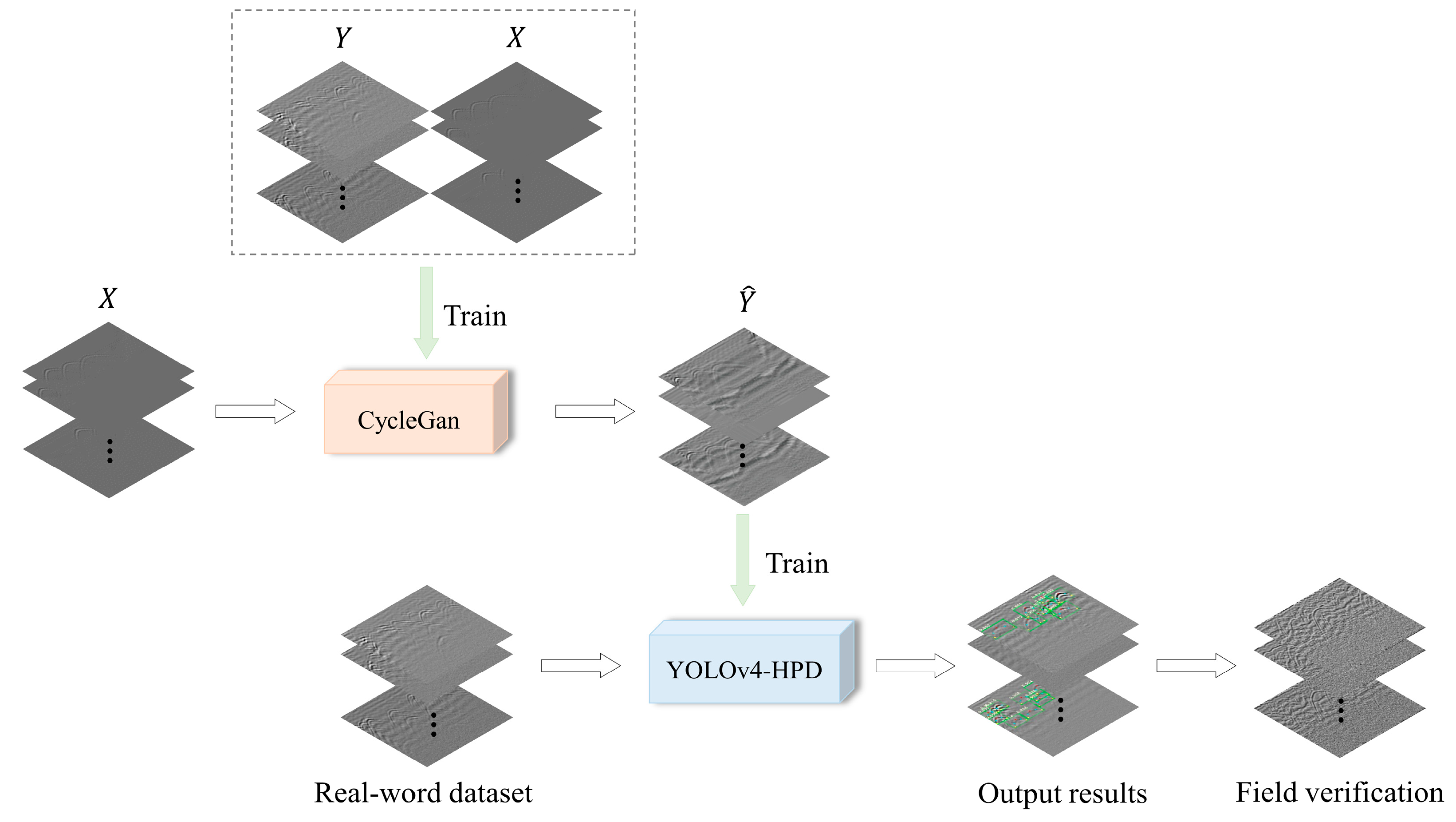
2. Materials and Methods
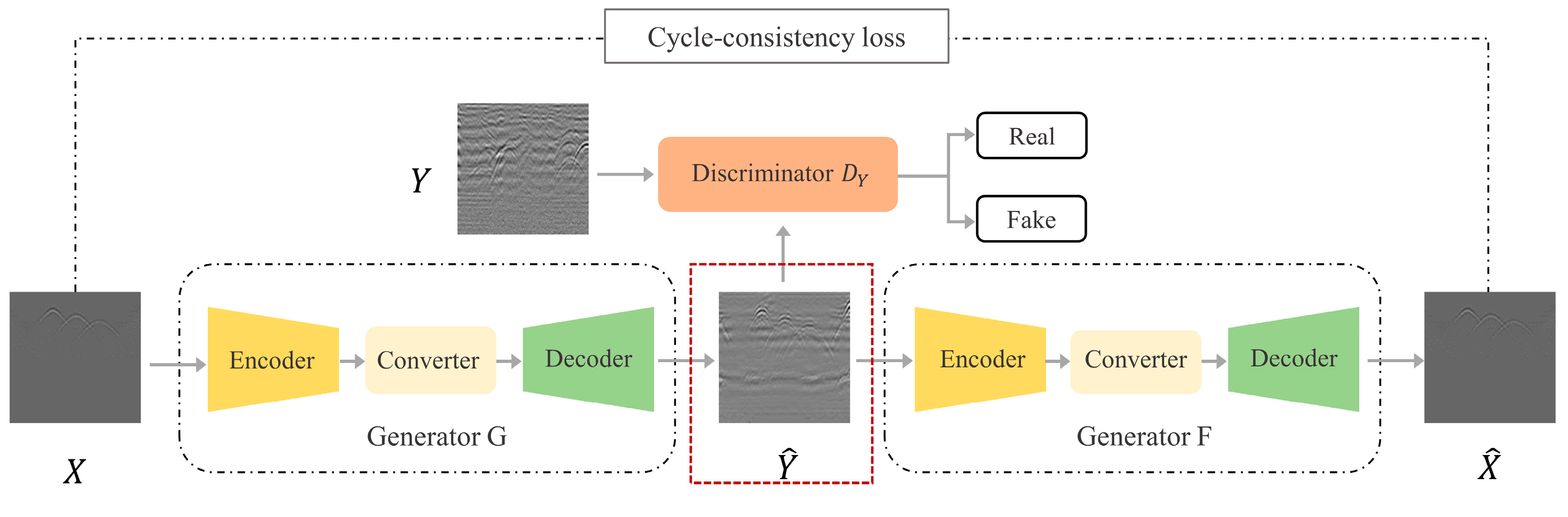
2.1. CMT-Net Model
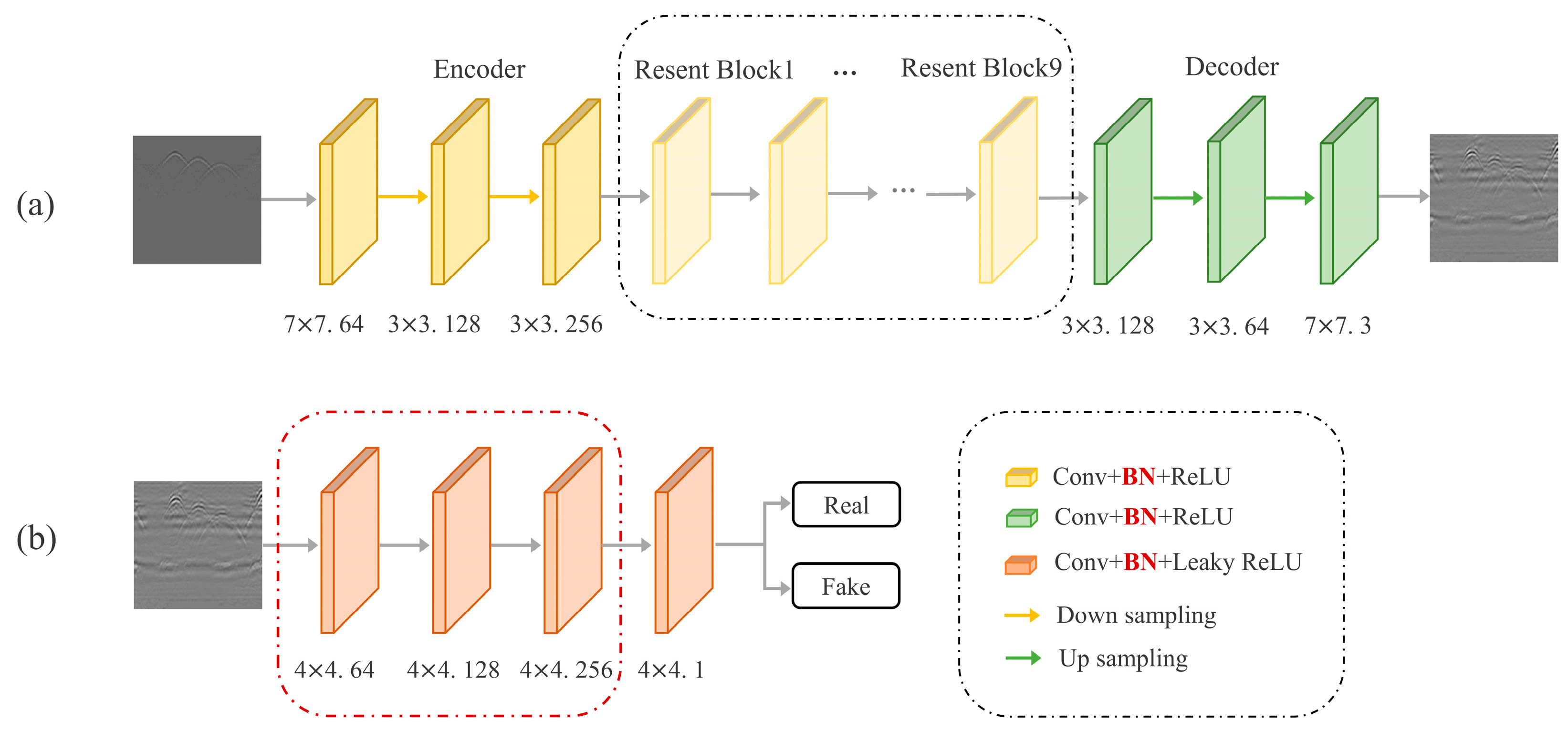
2.1.1. CycleGAN
- Since the source domain image and the target domain image used in this study are vastly dissimilar, the discriminator can easily distinguish between true and false images, making the network susceptible to training failure. To address this issue, the study reduces the sensitivity of the discriminator by reducing one layer of the convolutional layer.
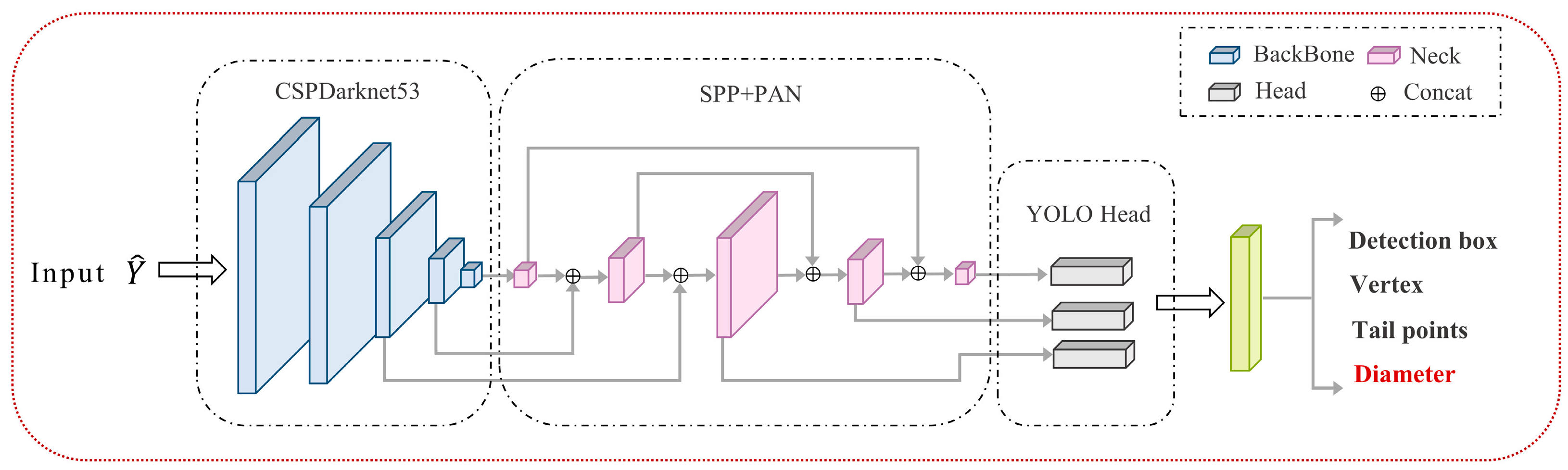
2.1.2. YOLOv4-HPD
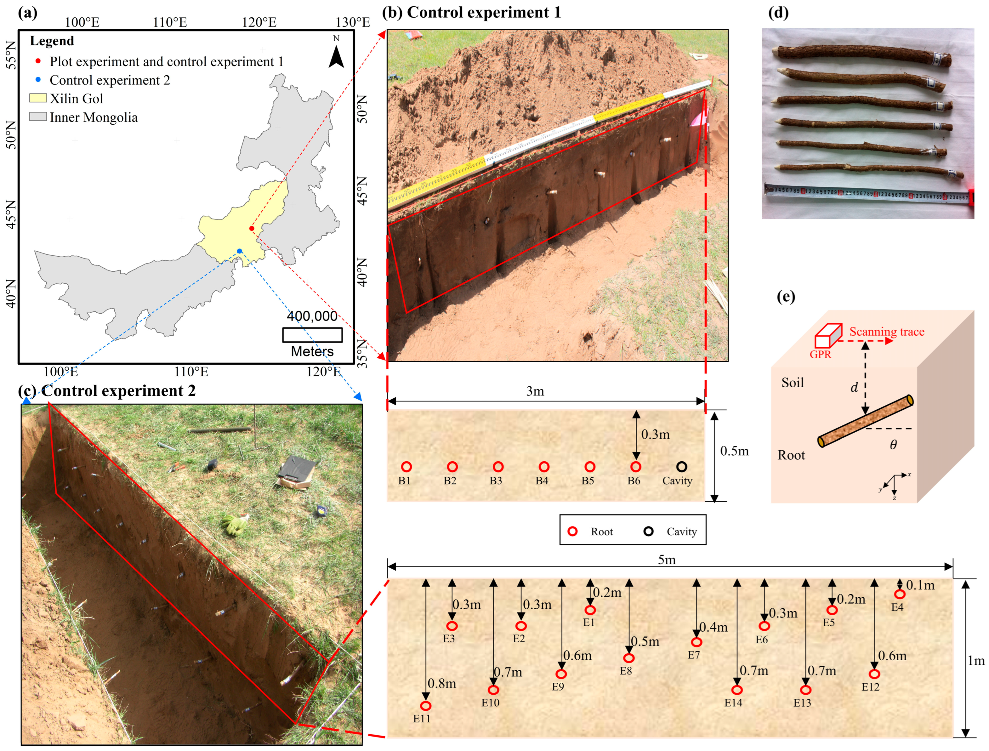
2.2. Data Description
2.2.1. Field Datasets
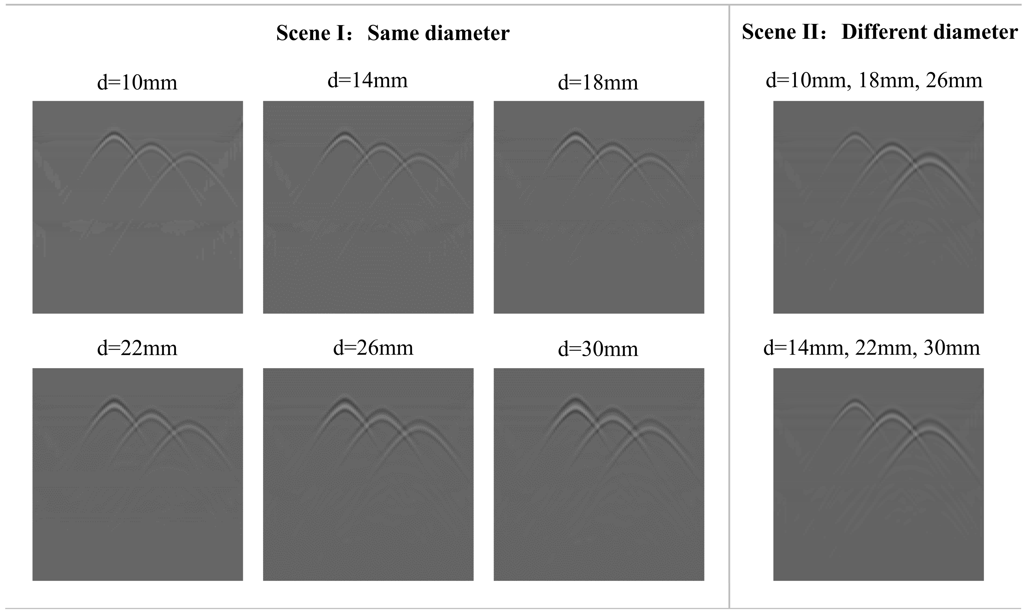
2.2.2. Synthetic Datasets
2.3. Experimental Setup and Evaluation Metrics
3. Results
3.1. Domain Migration Results by CycleGAN
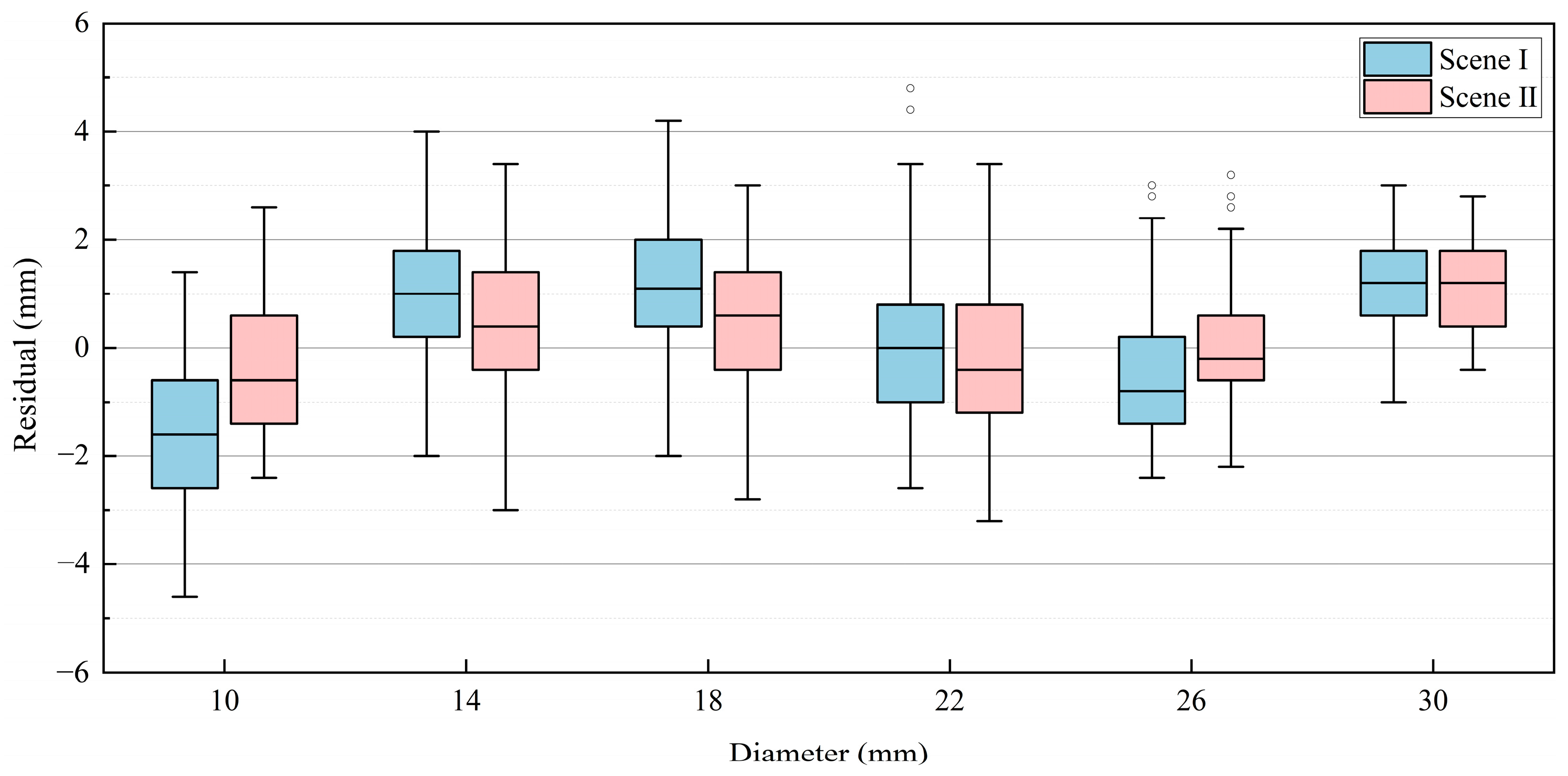
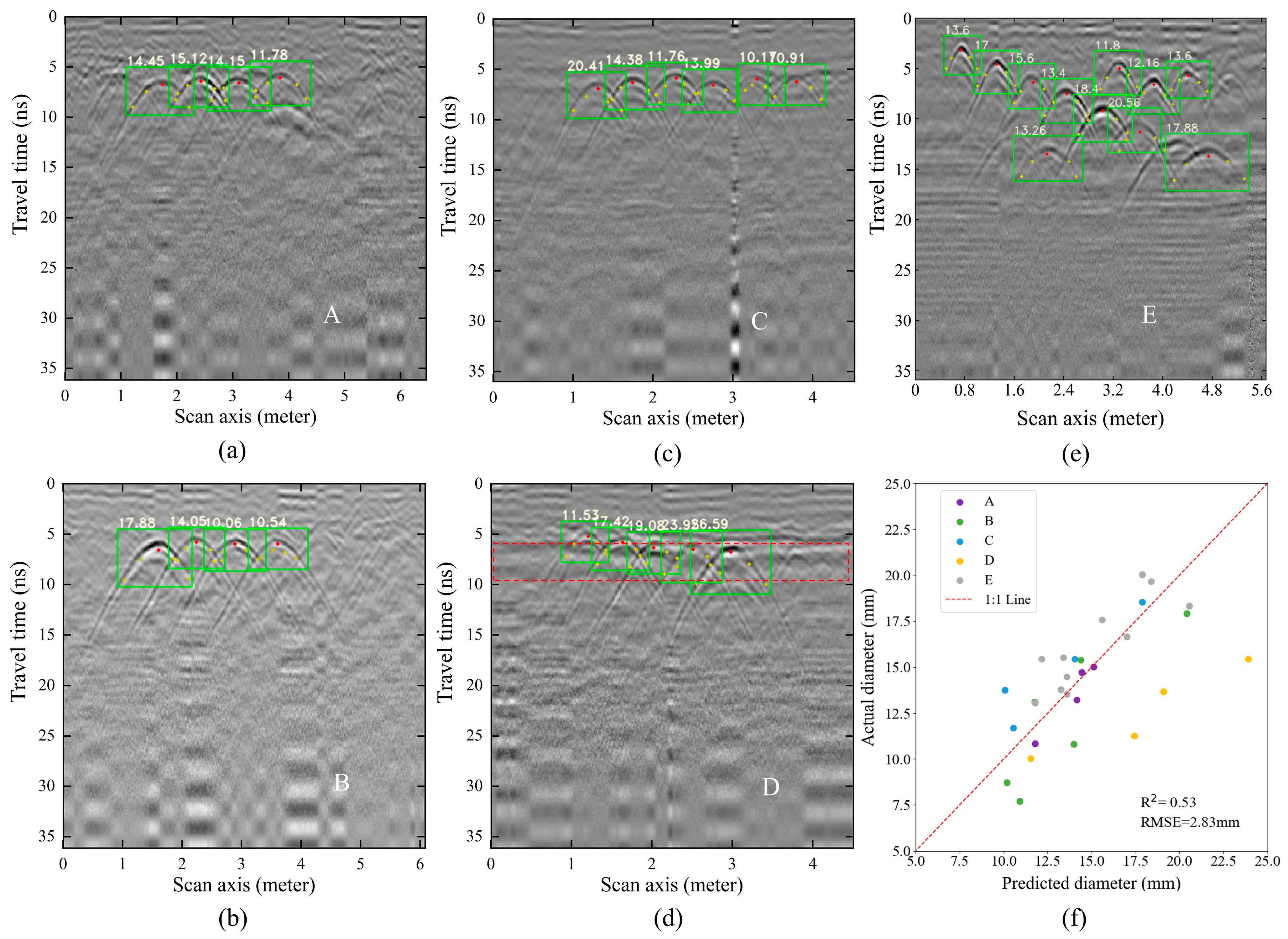
3.2. Root Diameter Estimation by YOLOv4-HPD
3.3. Model Generalization Verification
4. Discussion
4.1. Effectiveness of the Proposed CMT-Net Model
4.2. Comparison with Other Methods
4.3. Potential Applications of CMT-Net
4.4. Limitations and Future Outlook
5. Conclusions
Author Contributions
Funding
Data Availability Statement
Acknowledgments
Conflicts of Interest
References
- Brunner, I.; Godbold, D.L. Tree Roots in a Changing World. J. For. Res. 2007, 12, 78–82. [Google Scholar] [CrossRef]
- Gill, R.A.; Jackson, R.B. Global Patterns of Root Turnover for Terrestrial Ecosystems. New Phytol. 2000, 147, 13–31. [Google Scholar] [CrossRef]
- Yamase, K.; Tanikawa, T.; Dannoura, M.; Ohashi, M.; Todo, C.; Ikeno, H.; Aono, K.; Hirano, Y. Ground-Penetrating Radar Estimates of Tree Root Diameter and Distribution under Field Conditions. Trees 2018, 32, 1657–1668. [Google Scholar] [CrossRef]
- Metzner, R.; Eggert, A.; van Dusschoten, D.; Pflugfelder, D.; Gerth, S.; Schurr, U.; Uhlmann, N.; Jahnke, S. Direct Comparison of MRI and X-Ray CT Technologies for 3D Imaging of Root Systems in Soil: Potential and Challenges for Root Trait Quantification. Plant Methods 2015, 11, 17. [Google Scholar] [CrossRef] [PubMed]
- Cui, X.; Guo, L.; Chen, J.; Chen, X.; Zhu, X. Estimating Tree-Root Biomass in Different Depths Using Ground-Penetrating Radar: Evidence from a Controlled Experiment. IEEE Trans. Geosci. Remote Sens. 2013, 51, 3410–3423. [Google Scholar] [CrossRef]
- Nadezhdina, N.; Cermak, J. Instrumental Methods for Studies of Structure and Function of Root Systems of Large Trees. J. Exp. Bot. 2003, 54, 1511–1521. [Google Scholar] [CrossRef]
- Norby, R.J.; Jackson, R.B. Root Dynamics and Global Change: Seeking an Ecosystem Perspective. New Phytol. 2000, 147, 3–12. [Google Scholar] [CrossRef]
- Barton, C.V.M.; Montagu, K.D. Detection of Tree Roots and Determination of Root Diameters by Ground Penetrating Radar under Optimal Conditions. Tree Physiol. 2005, 24, 1323–1331. [Google Scholar] [CrossRef]
- Jol, H.M. Ground Penetrating Radar: Theory and Applications, 1st ed.; Elsevier Science: Amsterdam, The Netherlands; Oxford, UK, 2009; ISBN 978-0-444-53348-7. [Google Scholar]
- Giannopoulos, A. Modelling Ground Penetrating Radar by GprMax. Constr. Build. Mater. 2005, 19, 755–762. [Google Scholar] [CrossRef]
- Chang, C.W.; Lin, C.H.; Lien, H.S. Measurement Radius of Reinforcing Steel Bar in Concrete Using Digital Image GPR. Constr. Build. Mater. 2009, 23, 1057–1063. [Google Scholar] [CrossRef]
- Shihab, S.; Al-Nuaimy, W. Radius Estimation for Cylindrical Objects Detected by Ground Penetrating Radar. Subsurf. Sens. Technol. Appl. 2005, 6, 151–166. [Google Scholar] [CrossRef]
- Muniappan, N.; Rao, E.P.; Hebsur, A.V.; Venkatachalam, G. Radius Estimation of Buried Cylindrical Objects Using GPR—A Case Study. In Proceedings of the 2012 14th International Conference on Ground Penetrating Radar (GPR), Shanghai, China, 4–8 June 2012; pp. 789–794. [Google Scholar]
- Ristic, A.V.; Petrovacki, D.; Govedarica, M. A New Method to Simultaneously Estimate the Radius of a Cylindrical Object and the Wave Propagation Velocity from GPR Data. Comput. Geosci. 2009, 35, 1620–1630. [Google Scholar] [CrossRef]
- Sun, D.; Jiang, F.; Wu, H.; Liu, S.; Luo, P.; Zhao, Z. Root Location and Root Diameter Estimation of Trees Based on Deep Learning and Ground-Penetrating Radar. Agronomy 2023, 13, 344. [Google Scholar] [CrossRef]
- Dolgiy, A.; Dolgiy, A.; Zolotarev, V. Optimal Radius Estimation for Subsurface Pipes Detected by Ground Penetrating Radar. In Proceedings of the International Conference on Ground Penetrating Radar, Columbus, OH, USA, 19–22 June 2006. [Google Scholar]
- Sun, H.-H.; Lee, Y.H.; Dai, Q.; Li, C.; Ow, G.; Yusof, M.L.M.; Yucel, A.C. Estimating Parameters of the Tree Root in Heterogeneous Soil Environments via Mask-Guided Multi-Polarimetric Integration Neural Network. IEEE Trans. Geosci. Remote Sens. 2022, 60, 5108716. [Google Scholar] [CrossRef]
- Liang, H.; Fan, G.; Li, Y.; Zhao, Y. Theoretical Development of Plant Root Diameter Estimation Based on GprMax Data and Neural Network Modelling. Forests 2021, 12, 615. [Google Scholar] [CrossRef]
- Saito, K.; Ushiku, Y.; Harada, T. Asymmetric Tri-Training for Unsupervised Domain Adaptation. arXiv 2017, arXiv:1702.08400. [Google Scholar]
- Morerio, P.; Cavazza, J.; Murino, V. Minimal-Entropy Correlation Alignment for Unsupervised Deep Domain Adaptation. arXiv 2017, arXiv:1711.10288. [Google Scholar]
- Shu, Y.; Cao, Z.; Long, M.; Wang, J. Transferable Curriculum for Weakly-Supervised Domain Adaptation. In Proceedings of the AAAI Conference on Artificial Intelligence, Honolulu, HI, USA, 27 January–1 February 2019; Volume 33, pp. 4951–4958. [Google Scholar]
- Zhu, J.-Y.; Park, T.; Isola, P.; Efros, A.A. Unpaired Image-to-Image Translation Using Cycle-Consistent Adversarial Networks. In Proceedings of the 2017 IEEE International Conference on Computer Vision (ICCV), Venice, Italy, 22–29 October 2017; pp. 2242–2251. [Google Scholar]
- Giannakis, I.; Giannopoulos, A.; Warren, C. A Machine Learning Scheme for Estimating the Diameter of Reinforcing Bars Using Ground Penetrating Radar. IEEE Geosci. Remote Sens. Lett. 2021, 18, 461–465. [Google Scholar] [CrossRef]
- Hou, F.; Lei, W.; Li, S.; Xi, J. Deep Learning-Based Subsurface Target Detection from GPR Scans. IEEE Sens. J. 2021, 21, 8161–8171. [Google Scholar] [CrossRef]
- Pham, M.-T.; Lefèvre, S. Buried Object Detection from B-Scan Ground Penetrating Radar Data Using Faster-RCNN. In Proceedings of the IGARSS 2018—2018 IEEE International Geoscience and Remote Sensing Symposium, Valencia, Spain, 22–27 July 2018; pp. 6804–6807. [Google Scholar]
- Isola, P.; Zhu, J.-Y.; Zhou, T.; Efros, A.A. Image-to-Image Translation with Conditional Adversarial Networks. In Proceedings of the 2017 IEEE Conference on Computer Vision and Pattern Recognition (CVPR), Honolulu, HI, USA, 21–26 July 2017; pp. 5967–5976. [Google Scholar]
- Song, Y. Instance Normalization: The Missing Ingredient for Fast Stylization. arXiv 2017, arXiv:1607.08022. [Google Scholar]
- Ioffe, S.; Szegedy, C. Batch Normalization: Accelerating Deep Network Training by Reducing Internal Covariate Shift. In Proceedings of the 32nd International Conference on Machine Learning, PMLR, Lille, France, 6–11 June 2015; pp. 448–456. [Google Scholar]
- Li, S.; Cui, X.; Guo, L.; Zhang, L.; Chen, X.; Cao, X. Enhanced Automatic Root Recognition and Localization in GPR Images through a YOLOv4-Based Deep Learning Approach. IEEE Trans. Geosci. Remote Sens. 2022, 60, 5114314. [Google Scholar] [CrossRef]
- Bochkovskiy, A.; Wang, C.-Y.; Liao, H. YOLOv4: Optimal Speed and Accuracy of Object Detection. arXiv 2020, arXiv:2004.10934. [Google Scholar]
- Wang, C.-Y.; Mark Liao, H.-Y.; Wu, Y.-H.; Chen, P.-Y.; Hsieh, J.-W.; Yeh, I.-H. CSPNet: A New Backbone That Can Enhance Learning Capability of CNN. In Proceedings of the 2020 IEEE/CVF Conference on Computer Vision and Pattern Recognition Workshops (CVPRW), Seattle, WA, USA, 14–19 June 2020; pp. 1571–1580. [Google Scholar]
- Liu, S.; Qi, L.; Qin, H.; Shi, J.; Jia, J. Path Aggregation Network for Instance Segmentation. In Proceedings of the 2018 IEEE/CVF Conference on Computer Vision and Pattern Recognition, Salt Lake City, UT, USA, 18–23 June 2018; pp. 8759–8768. [Google Scholar]
- He, K.; Zhang, X.; Ren, S.; Sun, J. Spatial Pyramid Pooling in Deep Convolutional Networks for Visual Recognition. IEEE Trans. Pattern Anal. Mach. Intell. 2015, 37, 1904–1916. [Google Scholar] [CrossRef] [PubMed]
- Zheng, Z.; Wang, P.; Liu, W.; Li, J.; Ye, R.; Ren, D. Distance-IoU Loss: Faster and Better Learning for Bounding Box Regression. AAAI 2020, 34, 12993–13000. [Google Scholar] [CrossRef]
- Feng, Z.-H.; Kittler, J.; Awais, M.; Huber, P.; Wu, X.-J. Wing Loss for Robust Facial Landmark Localisation with Convolutional Neural Networks. In Proceedings of the 2018 IEEE/CVF Conference on Computer Vision and Pattern Recognition, Salt Lake City, UT, USA, 18–22 June 2018; pp. 2235–2245. [Google Scholar]
- Zhao, H.; Gallo, O.; Frosio, I.; Kautz, J. Loss Functions for Image Restoration With Neural Networks. IEEE Trans. Comput. Imaging 2017, 3, 47–57. [Google Scholar] [CrossRef]
- Tzanis, A. matGPR Release 2: A Freeware MATLAB® Package for the Analysis & Interpretation of Common and Single Offset GPR Data. FastTimes 2010, 15, 17–43. [Google Scholar]
- Liu, X.; Cui, X.; Guo, L.; Chen, J.; Li, W.; Yang, D.; Cao, X.; Chen, X.; Liu, Q.; Lin, H. Non-Invasive Estimation of Root Zone Soil Moisture from Coarse Root Reflections in Ground-Penetrating Radar Images. Plant Soil 2019, 436, 623–639. [Google Scholar] [CrossRef]
- Cao, Z.; Hidalgo, G.; Simon, T.; Wei, S.-E.; Sheikh, Y. OpenPose: Realtime Multi-Person 2D Pose Estimation Using Part Affinity Fields. IEEE Trans. Pattern Anal. Mach. Intell. 2021, 43, 172–186. [Google Scholar] [CrossRef]
- Lei, W.; Hou, F.; Xi, J.; Tan, Q.; Xu, M.; Jiang, X.; Liu, G.; Gu, Q. Automatic Hyperbola Detection and Fitting in GPR B-Scan Image. Autom. Constr. 2019, 106, 102839. [Google Scholar] [CrossRef]
- Dannoura, M.; Hirano, Y.; Igarashi, T.; Ishii, M.; Aono, K.; Yamase, K.; Kanazawa, Y. Detection of Cryptomeria japonica Roots with Ground Penetrating Radar. Plant Biosyst. 2008, 142, 375–380. [Google Scholar] [CrossRef]
- Zhu, S.; Huang, C.; Su, Y.; Sato, M. 3D Ground Penetrating Radar to Detect Tree Roots and Estimate Root Biomass in the Field. Remote Sens. 2014, 6, 5754–5773. [Google Scholar] [CrossRef]
- Cui, X.; Chen, J.; Shen, J.; Cao, X.; Chen, X.; Zhu, X. Modeling Tree Root Diameter and Biomass by Ground-Penetrating Radar. Sci. China Earth Sci. 2011, 54, 711–719. [Google Scholar] [CrossRef]
- Butnor, J.R.; Samuelson, L.J.; Stokes, T.A.; Johnsen, K.H.; Anderson, P.H.; González-Benecke, C.A. Surface-Based GPR Underestimates below-Stump Root Biomass. Plant Soil 2016, 402, 47–62. [Google Scholar] [CrossRef]


| Depth (m) | Profile | Average Root Diameter (mm) | |||||||
|---|---|---|---|---|---|---|---|---|---|
| 1 | 2 | 3 | 4 | 5 | 6 | 7 | |||
| 0° | 0.3 | A | 9.68 | 14.73 | 15.02 | 13.22 | 10.84 | Cavity | 6.35 |
| B | 7.71 | 8.73 | 10.82 | 13.13 | 15.40 | 17.91 | Cavity | ||
| 30° | 0.2 | C | Cavity | 18.54 | 15.44 | 13.77 | 11.69 | 10.03 | 22.76 |
| D | 8.11 | 10.03 | 11.26 | 13.68 | 15.46 | 22.76 | Cavity | ||
| 1 | 2 | 3 | 4 | 5 | 6 | 7 | 8 | 9 | 10 | 11 | 12 | 13 | 14 | |
|---|---|---|---|---|---|---|---|---|---|---|---|---|---|---|
| Depth (m) | 0.2 | 0.2 | 0.3 | 0.1 | 0.2 | 0.3 | 0.4 | 0.5 | 0.6 | 0.7 | 0.8 | 0.6 | 0.7 | 0.7 |
| Average root diameter (mm) | 13.06 | 15.46 | 14.49 | 13.54 | 16.65 | 17.56 | 15.53 | 19.66 | 18.31 | 19.72 | 20.05 | 13.4 | 16.08 | 13.79 |
| Evaluation Indicators | Precision | Recall | F1 | ||
|---|---|---|---|---|---|
| Value of accuracy | 99.8% | 100.0% | 99.9% | 99.8% | 94.3% |
| Root | Diameter (mm) | Absolute Error (mm) | Relative Error (%) | MAE (mm) | |
|---|---|---|---|---|---|
| True Value | Prediction Value | ||||
| A2 | 14.73 | 14.45 | 0.28 | 1.90% | 0.56 |
| A3 | 15.02 | 15.12 | 0.10 | 0.67% | |
| A4 | 13.22 | 14.15 | 0.93 | 7.03% | |
| A5 | 10.84 | 11.78 | 0.94 | 8.67% | |
| B1 | 7.71 | 10.91 | 3.20 | 41.50% | 2.12 |
| B2 | 8.73 | 10.17 | 1.44 | 16.49% | |
| B3 | 10.82 | 13.99 | 3.17 | 29.30% | |
| B4 | 13.13 | 11.76 | 1.37 | 10.43% | |
| B5 | 15.40 | 14.38 | 1.02 | 6.62% | |
| B6 | 17.91 | 20.41 | 2.50 | 13.96% | |
| C2 | 18.54 | 17.88 | 0.66 | 3.56% | 1.73 |
| C3 | 15.44 | 14.05 | 1.39 | 9.00% | |
| C4 | 13.77 | 10.06 | 3.71 | 26.98% | |
| C5 | 11.69 | 10.54 | 1.15 | 9.84% | |
| D2 | 10.03 | 11.53 | 1.50 | 14.96% | 5.07 |
| D3 | 11.26 | 17.42 | 6.16 | 54.70% | |
| D4 | 13.68 | 19.08 | 5.40 | 39.47% | |
| D5 | 15.46 | 23.92 | 8.46 | 54.72% | |
| D6 | 22.76 | 26.59 | 3.83 | 16.82% | |
| E1 | 13.06 | 11.80 | 1.26 | 9.65% | 1.47 |
| E2 | 15.46 | 12.16 | 3.30 | 21.35% | |
| E3 | 14.49 | 13.60 | 0.89 | 6.14% | |
| E4 | 13.54 | 13.60 | 0.06 | 0.44% | |
| E5 | 16.65 | 17.00 | 0.35 | 2.10% | |
| E6 | 17.56 | 15.60 | 1.96 | 11.16% | |
| E7 | 15.53 | 13.40 | 2.13 | 13.72% | |
| E8 | 19.66 | 18.40 | 1.26 | 6.41% | |
| E9 | 18.31 | 20.56 | 2.25 | 12.29% | |
| E11 | 20.05 | 17.88 | 2.17 | 10.82% | |
| E14 | 13.79 | 13.26 | 0.53 | 3.84% | |
Disclaimer/Publisher’s Note: The statements, opinions and data contained in all publications are solely those of the individual author(s) and contributor(s) and not of MDPI and/or the editor(s). MDPI and/or the editor(s) disclaim responsibility for any injury to people or property resulting from any ideas, methods, instructions or products referred to in the content. |
© 2025 by the authors. Licensee MDPI, Basel, Switzerland. This article is an open access article distributed under the terms and conditions of the Creative Commons Attribution (CC BY) license (https://creativecommons.org/licenses/by/4.0/).
Share and Cite
Cui, X.; Li, S.; Zhang, L.; Peng, L.; Guo, L.; Cao, X.; Chen, X.; Yin, H.; Shen, M. Integrated Extraction of Root Diameter and Location in Ground-Penetrating Radar Images via CycleGAN-Guided Multi-Task Neural Network. Forests 2025, 16, 110. https://doi.org/10.3390/f16010110
Cui X, Li S, Zhang L, Peng L, Guo L, Cao X, Chen X, Yin H, Shen M. Integrated Extraction of Root Diameter and Location in Ground-Penetrating Radar Images via CycleGAN-Guided Multi-Task Neural Network. Forests. 2025; 16(1):110. https://doi.org/10.3390/f16010110
Chicago/Turabian StyleCui, Xihong, Shupeng Li, Luyun Zhang, Longkang Peng, Li Guo, Xin Cao, Xuehong Chen, Huaxiang Yin, and Miaogen Shen. 2025. "Integrated Extraction of Root Diameter and Location in Ground-Penetrating Radar Images via CycleGAN-Guided Multi-Task Neural Network" Forests 16, no. 1: 110. https://doi.org/10.3390/f16010110
APA StyleCui, X., Li, S., Zhang, L., Peng, L., Guo, L., Cao, X., Chen, X., Yin, H., & Shen, M. (2025). Integrated Extraction of Root Diameter and Location in Ground-Penetrating Radar Images via CycleGAN-Guided Multi-Task Neural Network. Forests, 16(1), 110. https://doi.org/10.3390/f16010110