Article

Satellite Image Fusion Airborne LiDAR Point-Clouds-Driven Machine Learning Modeling to Predict the Carbon Stock of Typical Subtropical Plantation in China

1
School of Information Science and Technology, Beijing Forestry University, Beijing 100083, China
2
Engineering Research Center for Forestry-Oriented Intelligent Information Processing of National Forestry and Grassland Administration, Beijing 100083, China
3
Guangxi Forest Ecological Monitoring Center, Nanning 530028, China
4
Beijing Institute of Surveying and Mapping, Beijing 100038, China
*
Authors to whom correspondence should be addressed.
Forests 2024, 15(5), 751; https://doi.org/10.3390/f15050751
Submission received: 19 March 2024 / Revised: 22 April 2024 / Accepted: 24 April 2024 / Published: 25 April 2024

Abstract

:
In the current context of carbon neutrality, afforestation is an effective means of absorbing carbon dioxide. Stock can be used not only as an economic value index of forest wood resources but also as an important index of biomass and carbon storage estimation in forest emission reduction project evaluation. In this paper, we propose a data-driven machine learning framework and method for predicting plantation stock based on airborne LiDAR + satellite remote sensing, and carried out experimental verification at the site of the National Forest emission reduction project in Southern China. We used step-up regression and random forest (RF) to screen LiDAR and Landsat 8 OLI multispectral indicators suitable for the prediction of plantation stock, and constructed a plantation stock model based on machine learning (support vector machine regression, RF regression). Our method is compared with traditional statistical methods (stepwise regression and partial least squares regression). Through the verification of 57 plantation field survey data, the accuracy of the stand estimation model constructed using the RF method is generally better (ΔR2 = 0.01~0.27, ΔRMSE = 1.88~13.77 m3·hm−2, ΔMAE = 1.17~13.57 m3·hm−2). The model evaluation accuracy based on machine learning is higher than that of the traditional statistical method, and the fitting R2 is greater than 0.91, while the fitting R2 of the traditional statistical method is 0.85. The best fitting models were all support vector regression models. The combination of UAV point clouds and satellite multi-spectral images has the best modeling effect, followed by LiDAR point clouds and Landsat 8. At present, this method is only applicable to artificial forests; further verification is needed for natural forests. In the future, the density and quality of higher clouds could be increased. The validity and accuracy of the method were further verified. This paper provides a method for predicting the accumulation of typical Chinese plantations at the forest farm scale based on the “airborne LiDAR + satellite remote sensing” data-driven machine learning modeling, which has potential application value for the current carbon neutrality goal of the southern plantation forest emission reduction project.

1. Introduction

Forests have received a lot of attention from researchers and policymakers as a nature-based solution to climate change mitigation. Plantations account for approximately 7% of the world’s forest area (about 294 million hectares) and play a key role in supplying wood products and absorbing carbon dioxide. Many countries and regions around the world have made major declarations to achieve carbon peak and carbon neutrality, and forest carbon sequestration has become a hotspot of CCER with huge market potential [1,2]. Forest abatement schemes typically convert stock into biomass and, combined with expansion factors, into carbon stocks again [3]. Plantation forests provide a growing forest stock that is directly linked to existing renewable wood resources and biomass energy under intensive management practices [4]. Forest stock is the total volume of a stand or growing population per unit area, which is an important index to calculate the economic value of forests, and can directly reflect the quantity and quality of forest resources [5]. Therefore, the establishment of effective methods and technical means to accurately estimate the stock of plantation is crucial for forest managers to find a balance between plantation timber production and carbon sink trading [6,7].
Existing forest stock estimation methods usually rely on labor-intensive field measurements to obtain the necessary parameters, such as DBH and tree height obtained through field surveys after sampling the target forest, which can incur expensive human resources and economic costs [8,9]. The sites selected may not accurately represent the entire project area [10,11]. Low-frequency estimation may lead to delays in detecting changes in forest growth conditions [12]. Therefore, the previous estimation methods have some limitations, such as time and effort, limited investigation area, etc. [13,14]. In the context of carbon neutrality, people urgently need a more efficient and intelligent method to timely and accurately quantify forest stock and better balance the relationship between the economic value of renewable plantation and the value of carbon sink [15,16].
With the increasing maturity of ML, unmanned aerial vehicle and satellite remote sensing technology, its intelligent and high spatiotemporal resolution characteristics provide a new technology for forest stock estimation. At present, Light Detection and Ranging (LiDAR) is considered as an effective means to acquire forest 3D structure information at a regional or landscape scale [17,18]. Zeng Weisheng built a stock estimation model based on airborne LiDAR point clouds with a multiple regression method, which demonstrated the effectiveness of the forest stock multiple regression model based on point clouds [19]. Dalla established four machine learning methods based on LiDAR to estimate forest parameters, among which the support vector regression algorithm performed best [20]. Jiang Diexuan built a machine learning model based on the height and density of airborne point clouds in two periods to achieve dynamic storage estimation. Airborne LiDAR, unmanned aerial vehicles and satellite remote sensing technologies can provide high spatio-temporal resolution data, but obtaining these data is often costly and limited by weather conditions and geographical location. This can result in limited time and space coverage for data acquisition [21]. Remote sensing technology solves the problem of stock estimation at the stand or regional scale, and stock estimation at the forest farm, provincial or national scale requires satellite remote sensing [22,23]. Remarkable progress has been made in forest stock estimation based on satellite remote sensing, and forest parameters are constructed to estimate stock by extracting spectral and texture features [24]. By developing or improving data preprocessing methods and machine learning methods, people try to integrate multiple data sources to improve the estimation accuracy [25,26]. While machine learning models perform well on specific data sets, their ability to generalize remains a challenge. The data sets on which the model is trained are often geographically limited, and the prediction accuracy of the model may decline when applied to different regions or different forest types. Naik conducted generalized linear modeling based on Sentinel-2, Rapid Eye and other multi-spectral data to evaluate the impact of time, spectrum and spatial capabilities of multi-spectral satellites on forest stock prediction, and the results showed that the model built based on multi-temporal data was more effective than the single temporal model [27].
To improve the precision and spatial scale of forest resource estimation, more and more attention has been paid to research methods such as the combination of unmanned aerial vehicle and satellite remote sensing, LiDAR feature fusion and spectral feature fusion [28,29]. Using Sentinel-2 multispectral, Resource-3 stereo imaging and airborne LiDAR data, Wenke Lin studied the ability of multi-source remote sensing to estimate forest stock in the north subtropical region, and pointed out the advantages of the Bayesian model in forest stock estimation in the case of small samples [30]. Campbell combined airborne point clouds and multi-spectral images to jointly retrieve forest biomass, and pointed out that combined multi-data sources are conducive to large-scale forest parameter estimation [31]. Yu proposed a method that combined multi-spectral satellite images and airborne laser scanning data to estimate the forest stock of larch in China, and used the random forest model for estimation, which proved that the method had certain applicability and high accuracy. In addition, the fusion of hyperspectral remote sensing and other data sources has also achieved some results in forest stock estimation [32]. Gao combined airborne point clouds and hyperspectral data, adopted a random forest screening method and constructed multiple stepwise regression to estimate forest above-ground biomass, and the results showed that the fusion of multi-source data could significantly improve the estimation accuracy of the model [33]. The RF model was used to estimate the forest stock, and the verification showed that the method had certain applicability and high accuracy [34,35]. Although multi-source data fusion has been proved to improve the estimation accuracy of the model, the fusion processing between different data sources is a complex process, which needs to solve the problems of spatial, temporal and spectral resolution mismatch. In future studies, addressing these limitations will be the key to improving the accuracy and reliability of forest stock estimation [36]. There is a need to further explore more cost-effective data acquisition methods, improve model generalization, simplify and optimize multi-source data fusion processes, enhance model transparency and interpretability, and develop model training strategies for limited sample sizes.
Data sources and types, modeling methods and forest types affect the accuracy and stability of stock estimation [37,38]. This paper proposes an accurate forest stock estimation method based on “ML + LiDAR + satellite”, and a research experiment of “sky and ground integration” was carried out at the site of a national plantation emission reduction project in southern China [39]. The results show that the ML method combined with multi-source remote sensing can enhance the modeling of forest stock resources [40]. The research objectives of this paper are as follows: (1) a high-precision estimation method of eucalyptus plantation stock based on airborne point clouds combined with Landsat 8 images was proposed. This method aims to enhance the accuracy of eucalyptus stock estimation beyond the capabilities of existing techniques. (2) The estimation parameters and non-parametric models of eucalyptus plantation stock at the forest farm scale were established. These models are expected to provide a robust framework for accurate stock estimation, facilitating better forest management and resource allocation. (3) A scheme for estimating the stock of eucalyptus plantation with multi-source data is provided. This scheme is intended to leverage the complementary strengths of various data sources, thereby improving the reliability and precision of the stock estimation process.

2. Materials and Methods

Our workflow mainly includes data acquisition and processing, remote sensing feature variable screening, accumulation model construction and evaluation analysis (Figure 1). The first step is data collection and processing, which involved performing a plantation plot survey. The average height, average DBH, etc., of the sample were counted and converted to obtain the stock volume of the sample. Airborne LiDAR scanning and processing. The characteristic variables of point clouds are extracted through preprocessing such as original point clouds splicing and de-noising. In Landsat 8 OLI multispectral image processing, multi-spectral characteristic variables are extracted via radiometric calibration and atmospheric correction. The second step is feature variable screening. The variable characteristics after pretreatment were screened using the stepwise method and RF method, respectively, and the combination of selected variables was used as the accumulation modeling parameter. The third step is the accumulation model construction and evaluation. Four methods including stepwise regression, partial least squares regression, RF regression and support vector regression were used to construct the model, and the accuracy of the model was analyzed and evaluated by combining the field investigation data.

2.1. Study Area

The study area is located in a state-owned high-peak forest farm (108°06′–108°31′ E, 22°51′–23°02′ N) in Xingning District, Nanning City, Guangxi Zhuang Autonomous Region, a typical subtropical plantation (Figure 2). The average annual temperature is about 21 °C, the average annual precipitation is 1200–1500 mm, and the relative humidity is 79%. It is a hilly landform with an elevation of 100–460 m and a slope of 6–35°. It has thick red soil, suitable for the growth of subtropical and tropical tree species, with a forest coverage rate of 87%. The main tree species are Cunninghamia lanceolata, Eucalyptus grandis × urophylla, Pinus massoniana, and so on. Among them, Cunninghamia lanceolata is a tall tree belonging to the Cupressaceae family. Eucalyptus grandis × urophylla is an evergreen tree of the genus Myrtaceae. It is a hybrid of Eucalyptus grandis and urophylla developed in Brazil. Pinus massoniana is an arboreal plant of the genus Pinaceae with reddish-brown bark and grayish-brown underparts.

2.2. Data Collection

2.2.1. Plot Data

In January–February 2018, we set up 71 eucalyptus plots in the study area, of which 57 plots were within the airborne LiDAR coverage range, including 20 m × 20 m, 25 m × 25 m, and 25 m × 50 m. By calculating the storage quantity of different scale plots, we can obtain the storage quantity of each plot. It is measured in m3/hm2, a value that represents the amount of stock grown per square hectare of land. Real-time Kinematic (RTK) technology was used to accurately locate the specimen and record the central and corner coordinates of the specimen. We measured the DBH and height of eucalyptus trees in the plot by means of DBH, laser height measuring instrument and tape, and calculated the average height, DBH, number of trees and total area of the plot. According to the allometric growth equation of eucalyptus in Guangxi, the volume of single timber was calculated, and the value of hectare stock at the sample plot scale was obtained [41]. The formula is as follows:
V P l o t = V H e c t a r e · S P l o t 10,000 .
In the formula, V P l o t is the hectare reserve of the sample land, V H e c t a r e is the hectare reserve calculated by the binary volume formula, and S P l o t is the plot area.

2.2.2. LiDAR Data

In this paper, LiDAR data acquisition was carried out in January 2018 using an airborne LiDAR scanner.
We used LiDAR360 software (https://www.lidar360.com/ (accessed on 18 March 2024), Beijing GreenValley Technology Co., Ltd., Beijing, China) to splice, de-noise, classify ground points and normalize the collected point clouds (Figure A1). According to the longitude and latitude of the measured sample, the whole point clouds are cut into the sample site cloud. A total of 48 plot height and density variables were extracted based on point clouds (Table A1).

2.2.3. Landsat 8 Data

In this paper, multispectral images of Landsat 8 OLI, with track number P125/44 and a resolution of 30 m, were selected from the Gaofeng Forest farm area of Guangxi Province in February 2018. The image consists of 11 bands, bands 1 to 9 in the OLI Land Imager and bands 10 and 11 in the TIRS thermal infrared sensor. ENVI 5.31 software was used for radiometric calibration, atmospheric correction, image cropping, and so on. The FLASH atmospheric correction module was used for atmospheric correction of images after radiation calibration to eliminate the influence of atmospheric scattering and absorption. The image after radiometric calibration and atmospheric correction was cropped to obtain the image of the study area. Twenty-two band variables were extracted from the images in the study area, including 11 original band variables and 11 combined band variables. The original band feature variable factor was selected from band 1 to band 11 to highlight the rich image information and spectral characteristics. Based on the original band variable, 11 band combination variables were extracted (Table A2). Information of 13 remote sensing vegetation index variables in the study area was extracted.

2.3. Feature Variable Screening

2.3.1. Stepwise Screening

(1)
Point clouds characteristic variables
The partial F-test was set for the point clouds features, and the threshold F-value (Fin) of the rejection domain was set to be greater than the rejection F-value (Fout). We set the critical value of Fin as 0.10 and its significance level as 90%, corresponding to the quantile of F distribution as F (1, n−2, 0.90), and n was the sample size, indicating that in the current variable set, the newly added variable is added to the feature set when the significance level of the linear relationship between the newly added variable and the dependent variable is less than 0.1. The critical value of Fout was 0.11, the significance level was 89%, and the quantile of its F distribution was (1, n−2, 0.89), which represents the quantile of the corresponding F distribution under 1 and N-2 degrees of freedom and the significance level of 0.89. When a variable is deleted from the feature set, the significance level of the linear relationship between the residual variable and the dependent variable is greater than the significance level corresponding to 0.11, and the variable is deleted. The set of retained characteristic variables was D9, HP95, Hmax and Hkurtosis, including 1 density variable and 3 height variables. Multicollinearity testing was carried out on the combination of the aforementioned variables, and the Variance Inflation Factor (VIF) value between the two variables was calculated, respectively. The combination of variables with a VIF value greater than 10 was selected and the combination of variables was preferred. The VIF value between Hmax and HP95 was 250.25, much higher than the set threshold of 10, indicating a high degree of collinearity between the two variables (Table A3).
Two multivariate linear models, Y1 and Y2, were constructed with D9, Hmax, and Hkurtosis and D9, HP95, and Hkurtosis as modeling factors, respectively. The evaluation results are shown in Table A4; SE represents the standard estimation error. A better combination of variables was selected, and D9, Hmax, and Hkurtosis were finally selected as the screening results of the point clouds stepwise screening method. The coefficients of the parameters in the following equation are the fitting coefficients of the regression model in MATLAB 2023.
Y 1 = 470.232 D 9 + 4.897 H p 95 + 1.453 H k u r t o s i s 56.903
Y 2 = 482.214 D 9 + 4.855 H m a x + 1.461 H k u r t o s i s 65.01
(2)
Multispectral image feature variables
If the image resolution is lower than that of the point clouds, the feature variables cannot be screened if the Fin threshold is the same as that of the point clouds. To avoid the exclusion of potentially useful feature variables due to screening conditions, the critical value of Fin is set as 0.20, Fout as 0.21, and its significance level as 80%, corresponding to the quantile of F distribution as F (1, n−2, 0.80), and n is the sample size. In the current set of variables, only when the significance level of the linear relationship between the newly added variable and the dependent variable is less than 0.2 will it be added to the feature set. The critical value of Fout is 0.21, its significance level is 79%, and the quantile of its F distribution is (1, n−2, 0.79), that is, the quantile corresponding to the F distribution under 1 and N-2 degrees of freedom and the significance level of 0.79; in other words, when a variable is deleted from the feature set, the significance level of the linear relationship between the residual variable and the dependent variable is greater than that corresponding to 0.21. The feature variable set contains 7 band variables, namely B2, B6, B10, B11, B47, B452, and B457. Bivariate correlation analysis was performed on the selected set of characteristic variables, and correlation coefficient R and VIF were calculated (Table A5). The VIF of variables B10 and B11 was 12.16, greater than the set threshold of 10, indicating a high degree of collinearity between the two.
To avoid the negative effect of multicollinearity on modeling, the screening set was divided into two groups, using B2, B6, B10, B47, B452, and B457 and B2, B6, B11, B47, B452, and B457 as modeling factors to construct two multivariate linear models, Y3 and Y4. The better combination of the two variables was selected to compare the performance of the model constructed using the two component module factors (Table A6). Finally, B2, B6, B11, B47, B452, and B457 were selected as the screening results of multispectral images based on the stepwise screening method.
Y 3 = 674.932 B 47 0.051 B 6 + 0.870 B 2 + 4193.472 B 452 2425.697 B 457 + 0.018 B 10 10517.673
Y 4 = 2349.941 B 47 0.054 B 6 + 0.831 B 2 4142.719 B 452 2349.941 B 457 + 0.054 B 11 10834.272

2.3.2. Random Forest Screening

(1)
Point clouds characteristic variables
When the cumulative variance contribution of variables screened using the random screening method is greater than 90%, it is representative enough. We use MATLAB to obtain the importance ranking of 48 feature variables of point clouds and the proportion of cumulative feature contribution. When the cumulative feature contribution ratio is greater than 90%, a total of 29 feature variables are selected, and a large number of variables are retained as candidate factors. The threshold of feature variance contribution was set as 0.25, which showed good performance in multiple tests. Features larger than this threshold was selected as the screening results of the RF screening method (Figure A2), and Hcurt_m, D8, Hp30, and HA50 were selected as modeling factors.
(2)
Image feature variables
The importance of 35 feature variables of the image was sorted, the cumulative feature contribution ratio of the feature variables was calculated according to the ranking, and the threshold value of contribution ratio greater than 90% was set.
When the cumulative feature contribution ratio reached 90%, four image features were selected, namely B6, B7, GNDVI, and B5 (Figure A3). In the random forest screening method, these variables already contain 96% of the remote sensing information, so these variables are used for stock modeling.
The feature variables of point clouds and image were screened using SS and RFFS. The screening results of different methods are correlated to a certain extent. The screening results of point clouds features all contain 1 density variable and 3 height variables, and the top 2 variables are the canopy height variable and density variable. Both of the image screening results contain B6. The two data sources underwent variable screening through different screening methods, and the screening results were used as modeling factors for the subsequent construction of the accumulation model. To distinguish filter results for different data sources and different filtering methods, they have been renamed (see Table A7).

2.4. Accumulation Modeling Based on Point Clouds and Multispectral Images

Based on point clouds and multi-spectral images, we used parametric methods (stepwise regression, partial least squares regression) and non-parametric methods (support vector regression, RF regression) to construct a prediction model of eucalyptus plantation stock. The leave-one method cross-validation was used to assess and estimate the forest stock of the plot. Finally, the accuracy of the model was evaluated and analyzed with the field survey data of 57 eucalyptus plantations.

2.4.1. Stepwise Regression Modeling

To construct a stepwise regression model, it is not necessary to screen the feature variables repeatedly, and the selected variables are directly added to the stepwise regression model for multiple linear fitting. The point clouds variable combinations COLL1 and COLL2 were divided into training samples and verification samples according to the ratio of 9:1 using the leave-one method, respectively.
For the Landsat 8 image variable combinations COLL3 and COLL4 that have been screened out by us, a step-up regression model was constructed via cross-validation using the one-leave method, respectively.
Point clouds variable combination COLL5 and remote sensing image variable combination COLL6 were used to construct stepwise regression models using leave-one cross-validation, respectively.

2.4.2. Partial Least Squares Regression Modeling

The condition for extracting principal components was the measurement factor Q2h ≥ 0.975; that is, the principal components whose cumulative contribution rate was greater than 97.5% were retained until the extraction of principal components was stopped. After counting the number of principal components, the linear expression of independent variables and dependent variables is established, and the PLSR model is obtained using the established principal components. The PLSR model was constructed using the idea of leave-one-method cross-validation. The fitting parameter coefficients, constant terms and extracted principal component numbers of point clouds variable combinations COLL1 and COLL2 and Landsat 8 remote sensing image variable combinations COLL3 and COLL4 were calculated.
The fitting parameter coefficients and constant terms of Landsat 8 remote sensing image variable combinations COLL3 and COLL4 and the extracted number of principal components were calculated.
The results of fitting parameter coefficients and constant terms of COLL5 and COLL6 and the number of extracted principal components were obtained.

2.4.3. Random Forest Regression Modeling

In this paper, an RF regression model is constructed based on Baggerer (ensemble learning method). To determine the optimal parameter combination of the model, the grid search method was used to optimize the number of decision trees and the minimum number of leaf points. The number of decision trees ranged from 50 to 500 and the step size was 50. The minimum leaf count ranged from 2 to 10, with a step size of 1. By cross-verifying and evaluating each parameter combination, the mean square error (MSE) of the corresponding out-of-pocket error (OOB) for each parameter combination is calculated as follows:
M S E O O B = 1 n i = 1 n y i y i ^ 2
where y i is the true response value of the i th sample, y i ^ is the response value predicted on the out-of-pocket dataset using the RF regression model, and n is the number of samples in the out-of-pocket dataset.

2.4.4. Support Vector Regression Modeling

SVR includes linear, polynomial, RBF, sigmoid and other common kernel functions. We use the RBF kernel function to deal with complex nonlinear fitting between characteristic variable and accumulation. The grid search method is used to optimize the parameters of penalty coefficients C and gamma in the model. The values of C and gamma are 2 i , i 4,4 , respectively. The parameter combination with the highest average accuracy of model fitting is selected, and the stability and generalization ability of the model are further guaranteed using leave-one method cross-validation. According to the results of parameter optimization, the optimal penalty coefficient and gamma value were selected to construct the RBF-SVR model. The prediction results were compared with the measured accumulation in the plot to compare the goodness of fit of the model (as shown in Table A8).

2.5. Evaluation Index

In this study, R2, RMSE and MAE were used to quantitatively verify and evaluate the accuracy of the stand stock estimation model. R2 assesses the quality of the model’s fitted data, with values ranging from 0 to 1, with a value closer to 1 indicating better fitting of the model. RMSE can be used to measure the average difference between the model predicted value and the true value, where the smaller the MSE value, the smaller the dispersion degree between the true value and the model predicted value. MAE is a measure of the average absolute difference between the predicted value and the true value, where the smaller the MAE value, the smaller the error between the true value and the model predicted value.
R 2 = 1 i = 1 n y i y ^ i 2 i = 1 n y i y ¯ i 2
R M S E = i = 1 n y i y ^ i 2 n
M A E = 1 n i = 1 n y i y ^ i
where y i , y ¯ i , and y ^ i are the measured stock value, the average measured stock value, and the model predicted stock value, respectively, and n is the number of verification samples.

3. Results

According to the results of the stepwise screening method (SS) and random forest screening method (RFFS), the parameters of stepwise regression (SS), partial least squares regression (PLSR), random forest regression (RFR) and support vector regression (SVR) were optimized, and the leave-one method was used for cross-validation. The results of accumulation modeling under multi-data sources and multi-modeling methods were evaluated comprehensively by comparing the sample survey data with the model prediction.

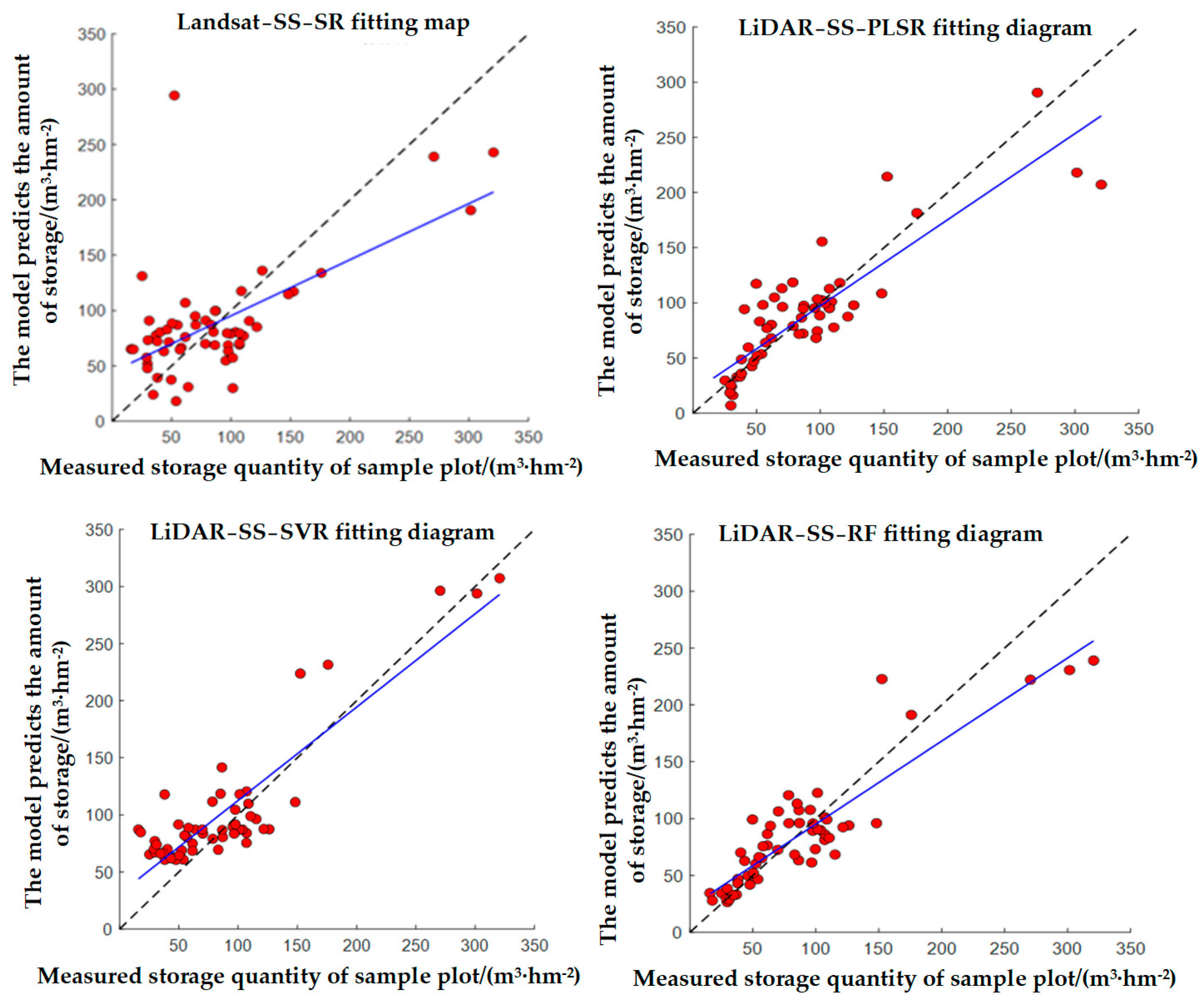
3.1. Point Clouds Model Evaluation and Analysis

The results are shown in Figure 3 and Figure 4. The solid line is the fitting line between the real value and the predicted value, and the dotted line is the 1:1 auxiliary judgment line. The blue line is the fitting line.
To comprehensively evaluate the model, R2, RMSE and MAE were used to comprehensively evaluate the above eight models; the results are shown in Table 1.
Based on the evaluation results of the above model, the following conclusions can be drawn:
(1)
The fitting accuracy of COLL2 optimized using random forest screening is generally better than that of COLL1 with stepwise regression. In addition to the stepwise regression method, other modeling methods can achieve better prediction results when using the random forest screening method. Among them, partial least squares regression, random forest regression and support vector regression can achieve better prediction results when using the random forest screening method. Compared with the stepwise screening method, R2 increased by 0.01~0.07, RMSE decreased by 1.88~6.11 m3·hm−2, MAE decreased by 2.04~7.25 m3·hm−2, and the SVR model had the most significant reduction in prediction error. R2 increased by 0.04, RMSE decreased by 6.11 m3·hm−2, MAE decreased by 7.25 m3·hm−2, and the stepwise regression method was more suitable for the COLL1 selected using the stepwise screening method.
(2)
The fitting effect of the non-parametric method is better than that of the parametric method. In this chapter, two non-parametric methods, random forest regression and support vector regression, constructed based on laser point clouds, have R2 values greater than or close to 0.9, and their RMSE and MAE evaluation indexes are small. In contrast, both partial least squares regression and stepwise regression in the parametric method have R2 values lower than 0.8, while the optimal parametric method model has an R2 values of only 0.83, and the corresponding RMSE and MAE indexes are relatively high.
It can be seen that when constructing a forest stock estimation model based on airborne LiDAR point clouds, using a random forest screening method and a constructing non-parametric method has the best model effect compared with other methods.

3.2. Evaluation and Analysis of Optical Remote Sensing Models

Figure 5 and Figure 6 show image-based forest stock modeling; the solid line is the fitting line between the true value and the predicted value, and the dashed line is the 1:1 auxiliary judgment line.
Table 2 shows the comprehensive evaluation of the eight models.
The specific model construction is as follows: support vector regression algorithms constructed based on different screening methods have high fitting accuracy, with the R2 reaching 0.62 and 0.67, respectively, but RMSE and MAE are also relatively high, with values of 60.86 m3·hm−2 and 46.20 m3·hm−2 and 54.64 m3·hm−2 and 32.63 m3·hm−2, respectively. Among the parametric methods, the model estimation error of the stepwise regression algorithm based on the COLL3 variable combination is the smallest, with an R2 of 0.66, RMSE of 35.76 m3·hm−2 and MAE of 29.01 m3·hm−2.
From the perspective of screening methods, when the COLL4 variable combination selected using the random forest screening method is used in the four modeling methods, compared with the COLL3 variable combination selected by the stepwise screening method, the model fitting accuracy is improved to a certain extent. The R2 increased by 0.03~0.27, RMSE decreased by 6.22~13.77 m3·hm−2, and MAE decreased by 1.17~13.57 m3·hm−2, among which the stepwise regression algorithm improved the best fit. It can be seen that the selection of random forest as a remote sensing feature variable is more reliable.
From the perspective of modeling methods, when the COLL3 variable combination is used as the model modeling factor, the fitting accuracy of parametric methods (stepwise regression and partial least squares regression) is smaller than that of non-parametric methods (support vector regression and random forest regression), and the R2 of the optimal performance model PLSR is only 0.4, while that of non-parametric methods reaches at least 0.53. When the COLL4 variable combination is used as the model modeling factor, the fitting accuracies of the parametric method and non-parametric method only slightly differ, but SVR is still the model with the highest fitting accuracy. It can be seen that the non-parametric method (machine learning method) has certain advantages when constructing the storage estimation model based on remote sensing sources.

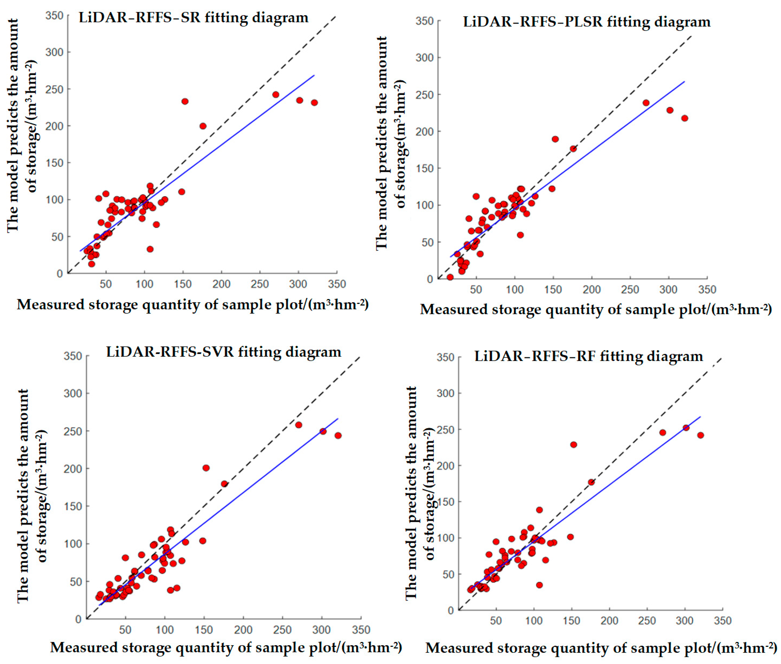
3.3. Model Evaluation and Analysis of Combined Point Clouds and Optical Remote Sensing

Forest stock modeling of point clouds combined with images is shown in Figure 7 and Figure 8.
(1)
According to the accuracy evaluation indexes of each model, it can be seen that the support vector regression model constructed based on the COLL6 variable combination of random forest screening method has the best prediction performance, with an R2 of 0.94, RMSE of 24.14 m3·hm−2 and MAE of 17.74 m3·hm−2. The results show that the combination of point clouds and optical remote sensing for forest stock inversion is feasible and can obtain better prediction results.
(2)
The modeling results based on the random forest screening method are better than the those obtained using the stepwise regression method. By comparing the model evaluation results when variable combination COLL5 and variable combination COLL6 were used in each modeling method, we can see that when variable combination COLL6 with the random forest screening method is used as the modeling factor, the overall prediction accuracy of each model is higher than that when COLL5 is used as the modeling factor, and the partial least squares model has the most significant improvement. The R2 increased by 0.08, the RMSE was 4.49 m3·hm−2, and the MAE was 2.69 m3·hm−2. Combined with the model evaluation results, it can be seen that when constructing forest stock estimation models based on single or multiple data sources, the random forest screening method is more reliable than the stepwise screening method as the feature variable screening method, and the combination of selected variables can better reflect the forest parameter information. The interpretation rate of the model after modeling can be improved more effectively.
(3)
The accuracy of non-parametric models (random forest regression and support vector regression) is better than that of parametric methods (stepwise regression and the partial least squares method). As can be seen from Table 3, among the eight models constructed by combining point clouds and optical remote sensing, the accuracy ranking of the models based on the combination of variables COLL5 and COLL6 is in the order of support vector regression, random forest regression, stepwise regression and partial least squares, and the top two are non-parametric methods. The fitting degree R2 values of the non-parametric methods established in this section are all greater than 0.91, while the best fitting result of the parametric methods is stepwise regression, whose fitting degree R2 is only 0.85, which is relatively low. According to the evaluation results of the model in Section 3.1 and Section 3.2, considering that the prediction of forest stock usually has certain nonlinear characteristics, the non-parametric method can capture these nonlinear relationships more flexibly, thus improving the prediction accuracy of the model. On the other hand, non-parametric methods can better deal with high-dimensional data and missing data problems. In the face of high dimensional data, non-parametric methods such as random forest regression can reduce the complexity of the model by constructing multiple decision trees, and at the same time have a good ability to deal with missing data. Therefore, the non-parametric method for retrieving forest stock has certain advantages over the parametric method.
(4)
Compared with the previous model using only a single data source, the prediction accuracy of the model combined with multiple data sources has been significantly improved. From the perspective of the dimensional evaluation model accuracy of the same screening method and the same modeling method, compared with only using point clouds, the model fit R2 increased by 0.01~0.09, RMSE decreased by 0.47~6.41 m3·hm−2, MAE decreased by 0.15~6.09 m3·hm−2, and the model accuracy improved more significantly than that using only optical remote sensing. The fit R2 increased by 0.19~0.46, RMSE decreased by 12.15~33.39 m3·hm−2, and MAE decreased by 10.55~26.34 m3·hm−2. According to the experimental results, combining multi-source data to build a forest stock model for forest stock inversion can significantly improve the prediction accuracy of the model. Under sufficient conditions, multi-data sources will be the first choice for modeling data sources.
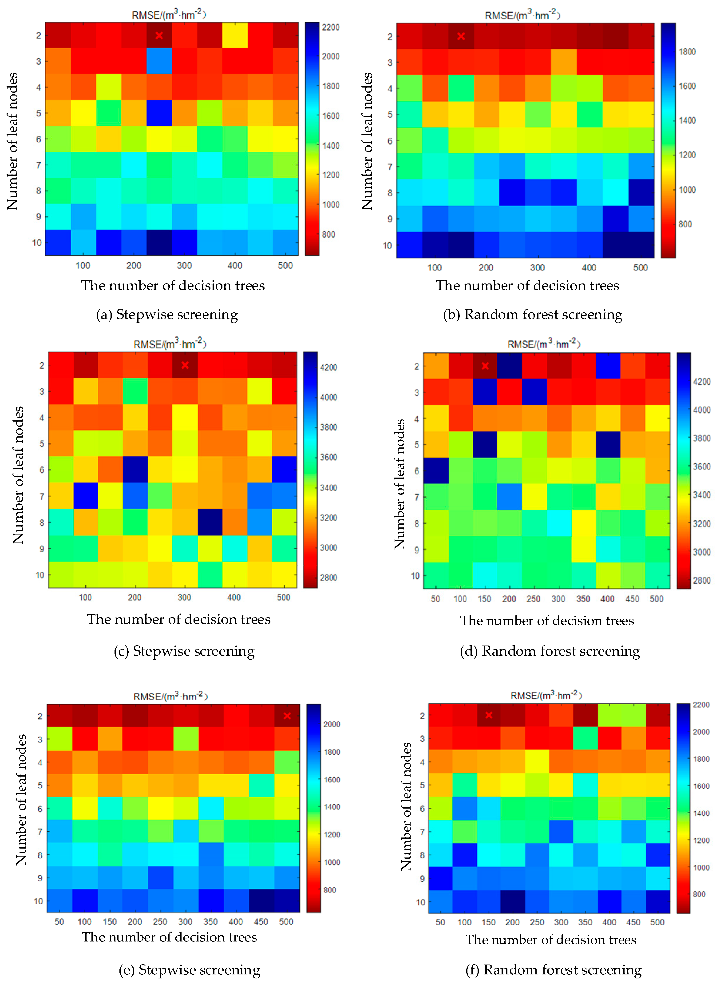
When the parameter combination corresponding to the minimum MSE of the out-of-pocket error is obtained during the optimization process, the value of the parameter combination is output to ensure the optimal prediction performance of the RF regression model. The model based on different data sources is cross-validated using the leave-one method. The results based on the combination of point clouds variables COLL1 and COLL2 are shown in Figure 9a,b. The optimal parameter combination is 2 and 250 and 2 and 150 as input parameters for modeling, respectively. The combination of spectral characteristic variables COLL3 and COLL4 is shown in Figure 9c,d, and the optimal parameter combination is 2 and 300 and 2 and 150, respectively. The modeling results of COLL5 and COLL6 are shown in Figure 9e,f, and the optimal parameter combinations are 2 and 500 and 2 and 150, respectively.

4. Discussion

4.1. Comparison of Parametric and Non-Parametric Methods in Modeling Plantation Stock

A forest stock estimation method based on “ML + LiDAR + satellite” was proposed in this paper. Based on the sample field survey data, LiDAR point clouds and satellite Landsat 8 OLI multi-spectral images, a modeling scheme combining single data source and multi-source data was constructed, respectively, and two screening methods (the step-up screening method and RF screening method) were used to screen the feature variables [42,43]. Based on parametric classical statistical methods (stepwise regression and partial least squares regression) and non-parametric ML methods (support vector regression and RF regression), a estimation model of eucalyptus plantation stock was constructed. Eight stock estimation models based on different variable screening methods and different modeling methods were constructed, respectively; and the accuracy of the methods ranged from high to low, as follows: support vector regression, RF regression, stepwise regression and partial least squares method. In terms of model construction methods, non-parametric methods have higher prediction accuracy than parametric methods do. In terms of evaluation indexes such as R2, RMSE and MAE, the non-parametric method showed a better prediction effect. It can be seen that the parametric method can better describe the complexity of forest ecosystem, and the parametric method can better deal with the noise in the data set and the nonlinear relationship of remote sensing. Thus, the generalization ability and stability of the model are improved. The results showed that support vector regression performed best among the four models, with an R2 of 0.94, RMSE of 24.14 m3·hm−2, and MAE of 17.74 m3·hm−2. Compared with the modeling of a single data source, the accuracy of the model based on multi-source data is significantly improved, with R2 increased by 0.01~0.09, RMSE decreased by 0.47~6.41 m3·hm−2, and MAE decreased by 0.15~6.09 m3·hm−2 compared with the point-cloud-based accumulation model. Therefore, in the case of sufficient conditions, selecting multiple data sources as modeling data sources will be the preferred choice to improve the prediction accuracy of forest stock inversion model. Compared with the model based on multispectral images, the accuracy of the model is improved more significantly, the fitting R2 is improved by 0.19~0.46, the RMSE is reduced by 12.15~33.39 m3·hm−2, and the MAE is reduced by 10.55~26.34 m3·hm−2. The model constructed with LiDAR point clouds can directly reflect the three-dimensional structural features such as the stand height and density, which is helpful to excavate the relationship between forest stock and characteristic variables. Whether it is UAV remote sensing or satellite remote sensing, the evaluation index shows considerable improvement. The estimation area of this paper is the forest farm scale. In the future, the research scope can be expanded to a regional or even global scale, and the forest stock estimation model under different time scales can be discussed [44,45]. In any case, under sufficient conditions, “ML + LiDAR + satellite” is the preferred method to estimate stock of eucalyptus plantation at the scale of forest farm.

4.2. Versatility of the Best Combination of Image and Point Clouds Features

According to the screening results of characteristic variables, it is shown that the point clouds height and density variables of forest canopy and the B6 band in multispectral images have significant effects on the estimation of forest stock. Secondly, by optimizing the parameters of the four regression models one by one, the estimation accuracy of different models is better. Finally, cross-validation of different storage estimation models is carried out by reserving one method, which makes the results more stable and reliable [46,47]. In terms of R2, RMSE, MAE and other evaluation indicators, ML methods (SVR, RF) have better prediction effect than statistical analysis methods (SS and PLSR) and can better describe the noise and nonlinear relations in the data set. When the random forest screening method is used to select modeling factors, the four models show better prediction accuracy, and can deal with high-dimensional data and nonlinear relations more effectively than the stepwise screening method. The prediction performance of the SVR model based on the COLL6 variable combination of the random forest screening method is the best, with an R2 of 0.94, RMSE of 24.14 m3·hm−2 and MAE of 17.74 m3·hm−2, indicating that airborne LiDAR and satellite remote sensing based on SVR can effectively estimate forest stock. When COLL6, the variable combination of random forest screening method, is used as the modeling factor, the overall prediction accuracy of all models is higher than that of COLL5, and the partial least squares model has the most significant improvement, with an increase of 0.08 in R2, 4.49 m3·hm−2 in RMSE and 2.69 m3·hm−2 in MAE. Wang used the CNN-LSTM-Attention model to predict forest stock, and its RMSE of 26.15 m3·hm−2 was slightly lower than our model [48]. Therefore, whether focused on a single-source or multi-source data, ML methods such as SVR and RF can more effectively improve the interpretation rate of the model.

4.3. Non-Parametric Approaches and Combined Data Oriented towards Carbon Neutrality Goals Can Improve Forest Volume Resource Modeling

Among the eight models constructed by combining point clouds and multi-spectral images, the accuracy of methods in COLL5 or COLL6 variable combination is, from high to low: support vector regression, random forest regression, stepwise regression and partial least squares; the first two are non-parametric ML methods. The fitting degree R2 of the non-parametric method is greater than 0.91, while the best fitting result of the parametric statistical analysis method is stepwise regression, whose fitting degree R2 is 0.85. The current problem of forest stock estimation has nonlinear characteristics, and the ML method can capture the nonlinear relationship more flexibly [49]. Non-parametric methods can better deal with the problem of missing high-dimensional data. For example, random forest regression can reduce the complexity of the model by constructing multiple decision trees. When constructing the accumulation model based on different data sources, the ML method represented by the SVR model performs best. The results show that the point clouds combined with Landsat 8 image is the best, followed by LiDAR point clouds, and Landsat 8 is the last. Multi-source data and non-parametric methods can improve the accuracy and stability of forest stock estimation model, have significant advantages in predicting forest stock, and can better deal with the noise in data sets and the nonlinear relationship of remote sensing.

4.4. Limitations and Future Directions

In this study, a machine learning framework combining airborne LiDAR and satellite remote sensing data is proposed for predicting plantation stock in southern China. The method has shown high accuracy and reliability in experimental verification. However, there are some limitations to the study. Firstly, the current method is mainly aimed at the application of planted forests. For natural forests, due to the complexity and diversity of their structures, the applicability and accuracy of this method need to be further verified. Secondly, airborne LiDAR has certain limitations in obtaining point clouds data of understory vegetation, which may affect the accuracy of estimation of understory biomass. Thirdly, although the machine learning model used in this study is based on traditional statistical methods, its universality and applicability under different stand conditions need to be further explored.
Considering the above limitations, future research could be carried out in the following directions. The scope of this study could be extended to natural forests. Different stand types and understory vegetation were considered to enhance the universality and applicability of the model. Moreover, the application of deep learning in forest stock estimation could be explored as deep learning models such as convolutional neural networks may have higher accuracy and efficiency in processing spatial data. The fusion of CNNs with LiDAR data and multispectral satellite images could be optimized for better forest analysis. This paper recommends increasing the density and quality of data collection to enhance understory vegetation scanning. CNNs can contribute by processing this denser data more efficiently [50]. At the same time, the scanning ability of understory vegetation can be improved by increasing the density and quality of high cloud to enhance the accuracy of the model to estimate the whole stand biomass. The fusion method of LiDAR data and satellite multi-spectral data can be further explored and optimized to improve the estimation accuracy of the model under different stand conditions. Finally, field validation can be carried out across a wider range of areas and different types of forests to assess the validity and applicability of the model, facilitating its application in real forest management and carbon stock assessment. Through research in the above directions, the forest stock estimation method based on airborne Lidar and satellite remote sensing could be further improved and optimized in the future to provide more accurate and effective scientific support for forest resource management and carbon neutrality goals.

5. Conclusions

This paper proposes a forest stock estimation method based on “ML + LiDAR + satellite”, which provides a promising tool for the assessment of wood resources in plantations under carbon neutrality targets. Based on a parametric statistical analysis method and non-parametric artificial intelligence method, the stock model of a eucalyptus plantation in southern China was constructed. The ML method can capture nonlinear relationships more flexibly. The following results were obtained: ΔR2 = 0.01~0.27, ΔRMSE = 1.88~13.77 m3·hm−2, and ΔMAE = 1.17~13.57 m3·hm−2. The current research methods are mainly aimed at artificial forests, and their applicability and accuracy have not been fully verified in natural forests. This study mainly adopts support vector machine regression and random forest regression methods. Although it has advantages compared with traditional statistical methods, it does not explore the application potential of more advanced machine learning algorithms such as deep learning in this field. In the future, we could try to adopt more advanced AI methods to expand the scope of research to a regional or even national scale. All in all, under the goal of carbon neutrality, how the machine learning modeling scheme can better serve the balance of wood resources and ecological services in plantation forests is one of the main questions for our future research.

Author Contributions

Conceptualization, G.F.; data curation, F.L., Y.W. and C.G.; formal analysis, G.F. and H.C.; investigation, J.Z., Q.X. and F.L.; methodology, G.F. and B.Z.; resources, W.L. and Y.W.; software, B.Z. and X.Z.; supervision, H.C. and Z.D.; visualization, J.Z.; writing—original draft, G.F.; writing—review and editing, R.W. All authors have read and agreed to the published version of the manuscript.

Funding

This research was funded by Key Research and Development Project of Inner Mongolia Autonomous Region (2022YFHH0065-03); Laibin Jinxiu Dayaoshan Forest Ecosystem Observation and Research Station Guangxi of under Grand (No. 22-035-130-01); Tibet Autonomous Region Science and Technology Plan Project (XZ202301YD0043C); Mangrove species identification and growth monitoring warning by integrating UAV hyperspectral images and LiDAR point clouds (2024GXLK08); National Guilin Scientific Research ([2022] No. 6); Postdoctoral Innovative Talent Support Program (BX20220038).

Data Availability Statement

Data will be made available on request.

Acknowledgments

We acknowledge the data support from the National Forestry and GrasslandScience Data Center (NFGSDC), National Science & Technology Infrastructure of China. (http://www.forestdata.cn (accessed on 1 November 2022)). We thank Zhuo Deng and all those who have made important contributions to this paper.

Conflicts of Interest

The authors declare no conflicts of interest.

Appendix A

Table A1. Extraction of airborne laser scanning (ALS) point clouds feature variables.
Variable TypeVariable NameFeature Description
Height
variable
HmaxThe maximum value of Z for all normalized points
HminThe minimum value of the Z-value of all normalized points
Hmedian_zAltitude mean deviation
HstddevHeight standard deviation
HkurtosisHeight kurtosis
Hsqrt_mHeight quadratic mean
Hcurt_mHeight cubic mean
HP1,HP5,…,HP99Normalized percentile of point cloud height distribution, a total of 15
HA1,HA2,…,HA99Normalized percentile of cumulative height of point clouds, a total of 15
Density
variable
D1,D2,…,D9The point clouds are divided into ten slices of the same height from low to high, and the proportion of echo points of the layer in all return points is 10 in total
Canopy
density
CCThe ratio of vegetation points to all points in the first echo
Table A2. Extract band variables of multispectral images.
Band CombinationEquation
B 24 B 2 / B 4
B 534 B 3 × B 4 / B 5
B 547 B 5 × B 4 / B 7
B 452 ( B 4 + B 5 B 2 ) / ( B 4 + B 5 + B 2 )
B 45 B 4 + B 5
B 75 B 7 / B 5
B 53 B 5 / B 3
B 345 B 3 + B 4 + B 5
V I S 234 B 2 + B 3 + B 4
B 47 B 4 / B 7
A l b e d o 0.356 B 1 + 0.130 B 3 + 0.373 B 4 + 0.085 B 5 + 0.072 B 7 0.0018
Table A3. VIF values between point clouds variables.
D9HmaxHP95Hkurtosis
D9-2.462.691.00
Hmax2.46-250.251.01
HP952.69250.25-1.01
Hkurtosis1.001.011.01-
Table A4. Preliminary evaluation of stepwise regression model for point clouds.
ModelR2Adjusted R2SE
Y10.9020.89418.460
Y20.9080.90017.904
Table A5. VIF values between remote sensing image variables.
B47B6B2B11B10B452B457
B47-4.431.081.311.222.171.09
B64.43-1.391.671.481.991.03
B21.081.39-1.491.411.001.00
B111.311.671.49-12.161.021.17
B101.221.481.4112.16-1.021.13
B4522.171.991.001.021.02-1.13
B4571.091.031.001.171.131.13-
Table A6. Preliminary evaluation of multivariate linear models for remote sensing images.
ModelR2Adjusted R2SE
Y30.4940.43446.618
Y40.5020.44246.272
Table A7. Summary screening results and variable combination naming.
Data SourceScreening MethodScreening ResultVariable Combination Naming
Point cloudsSSD9, HP95, Hmax, HkurtosisCOLL1
RFFSHcurt_m, D8, Hp30, HA50COLL2
Optical remote sensingSSB2, B6, B11, B47, B452, B457COLL3
RFFSB6, B7, GNDVI, B5COLL4
Point clouds combined with optical remote sensingSSCOLL1 + COLL3COLL5
RFFSCOLL2 + COLL4COLL6
Table A8. The prediction results were compared with the measured accumulation in the plot to compare the goodness of fit of the model.
CGammaC Optimum ValueGamma Optimum Value
COLL1 and COLL22 and 0.1258 and 0.1252 and 80.125
COLL3 and COLL48 and 0.1250.25 and 88 and 0.250.125 and 8
COLL5 and COLL68 and 0.1251 and 0.1258 and 10.125

Appendix B

Figure A1. Cloud processing results of sample locations. The height increases from blue to red, with blue representing the ground and red representing the forest canopy.
Forests 15 00751 g0a1
Figure A2. Point clouds feature variance contribution ranking chart. Set the dotted line as the feature variance contribution threshold to 0.25. Red is for variables greater than 0.25 and blue is for variables less than 0.25.
Forests 15 00751 g0a2
Figure A3. Remote sensing image feature variance contribution ranking chart. The cumulative feature contribution ratio of feature variables is calculated according to the ranking. The threshold value is set as the contribution ratio greater than 90%, and the red value is the cumulative feature contribution ratio greater than 90%. Blue is less than 90% of the cumulative feature contribution.
Forests 15 00751 g0a3

References

  1. Jayathunga, S.; Owari, T.; Tsuyuki, S. The Use of Fixed–Wing UAV Photogrammetry with LiDAR DTM to Estimate Merchantable Volume and Carbon Stock in Living Biomass over a Mixed Conifer–Broadleaf Forest. Int. J. Appl. Earth Obs. Geoinf. 2018, 73, 767–777. [Google Scholar] [CrossRef]
  2. Neeff, T.; de Alencastro Graça, P.M.; Dutra, L.V.; da Costa Freitas, C. Carbon Budget Estimation in Central Amazonia: Successional Forest Modeling from Remote Sensing Data. Remote Sens. Environ. 2005, 94, 508–522. [Google Scholar] [CrossRef]
  3. Qin, H.; Zhou, W.; Yao, Y.; Wang, W. Estimating Aboveground Carbon Stock at the Scale of Individual Trees in Subtropical Forests Using UAV LiDAR and Hyperspectral Data. Remote Sens. 2021, 13, 4969. [Google Scholar] [CrossRef]
  4. Wu, W.; Xu, L.; Zheng, H.; Zhang, X. How Much Carbon Storage Will the Ecological Space Leave in a Rapid Urbanization Area? Scenario Analysis from Beijing-Tianjin-Hebei Urban Agglomeration. Resour. Conserv. Recycl. 2023, 189, 106774. [Google Scholar] [CrossRef]
  5. Byrd, K.B.; Ballanti, L.; Thomas, N.; Nguyen, D.; Holmquist, J.R.; Simard, M.; Windham-Myers, L. A Remote Sensing-Based Model of Tidal Marsh Aboveground Carbon Stocks for the Conterminous United States. ISPRS J. Photogramm. Remote Sens. 2018, 139, 255–271. [Google Scholar] [CrossRef]
  6. Madundo, S.D.; Mauya, E.W.; Kilawe, C.J. Comparison of Multi-Source Remote Sensing Data for Estimating and Mapping above-Ground Biomass in the West Usambara Tropical Montane Forests. Sci. Afr. 2023, 21, e01763. [Google Scholar] [CrossRef]
  7. Smith, B.; Knorr, W.; Widlowski, J.-L.; Pinty, B.; Gobron, N. Combining Remote Sensing Data with Process Modelling to Monitor Boreal Conifer Forest Carbon Balances. For. Ecol. Manag. 2008, 255, 3985–3994. [Google Scholar] [CrossRef]
  8. Poorazimy, M.; Shataee, S.; McRoberts, R.E.; Mohammadi, J. Integrating Airborne Laser Scanning Data, Space-Borne Radar Data and Digital Aerial Imagery to Estimate Aboveground Carbon Stock in Hyrcanian Forests, Iran. Remote Sens. Environ. 2020, 240, 111669. [Google Scholar] [CrossRef]
  9. Zheng, Y.; Zhang, B. The Impact of Carbon Market on City Greening: Quasi-Experimental Evidence from China. Resour. Conserv. Recycl. 2023, 193, 106960. [Google Scholar] [CrossRef]
  10. Guo, Q.; Du, S.; Jiang, J.; Guo, W.; Zhao, H.; Yan, X.; Zhao, Y.; Xiao, W. Combining GEDI and Sentinel Data to Estimate Forest Canopy Mean Height and Aboveground Biomass. Ecol. Inform. 2023, 78, 102348. [Google Scholar] [CrossRef]
  11. Massetti, A.; Gil, A. Mapping and Assessing Land Cover/Land Use and Aboveground Carbon Stocks Rapid Changes in Small Oceanic Islands’ Terrestrial Ecosystems: A Case Study of Madeira Island, Portugal (2009–2011). Remote Sens. Environ. 2020, 239, 111625. [Google Scholar] [CrossRef]
  12. Ai, X.-N.; Gao, S.-J.; Li, W.-M.; Liao, H. Greening China: Environmentally Adjusted Multifactor Productivity in the Last Four Decades. Resour. Conserv. Recycl. 2023, 192, 106918. [Google Scholar] [CrossRef]
  13. Chaddad, F.; Mello, F.A.O.; Tayebi, M.; Safanelli, J.L.; Campos, L.R.; Amorim, M.T.A.; Barbosa de Sousa, G.P.; Ferreira, T.O.; Ruiz, F.; Perlatti, F.; et al. Impact of Mining-Induced Deforestation on Soil Surface Temperature and Carbon Stocks: A Case Study Using Remote Sensing in the Amazon Rainforest. J. S. Am. Earth Sci. 2022, 119, 103983. [Google Scholar] [CrossRef]
  14. Pereira, O.J.R.; Montes, C.R.; Lucas, Y.; Melfi, A.J. Use of Remote Sense Imagery for Mapping Deep Plant-Derived Carbon Storage in Amazonian Podzols in Regional Scale. In Proceedings of the 2013 IEEE International Geoscience and Remote Sensing Symposium—IGARSS, Melbourne, Australia, 21–26 July 2013; pp. 3770–3772. [Google Scholar]
  15. Chang, F.-C.; Ko, C.-H.; Yang, P.-Y.; Chen, K.-S.; Chang, K.-H. Carbon Sequestration and Substitution Potential of Subtropical Mountain Sugi Plantation Forests in Central Taiwan. J. Clean. Prod. 2017, 167, 1099–1105. [Google Scholar] [CrossRef]
  16. Zhou, P.; Sun, Z.; Zhang, X.; Wang, Y. A Framework for Precisely Thinning Planning in a Managed Pure Chinese Fir Forest Based on UAV Remote Sensing. Sci. Total Environ. 2023, 860, 160482. [Google Scholar] [CrossRef] [PubMed]
  17. Bordoloi, R.; Das, B.; Tripathi, O.P.; Sahoo, U.K.; Nath, A.J.; Deb, S.; Das, D.J.; Gupta, A.; Devi, N.B.; Charturvedi, S.S.; et al. Satellite Based Integrated Approaches to Modelling Spatial Carbon Stock and Carbon Sequestration Potential of Different Land Uses of Northeast India. Environ. Sustain. Indic. 2022, 13, 100166. [Google Scholar] [CrossRef]
  18. Yang, C.; Liu, J.; Zhang, Z.; Zhang, Z. Estimation of the Carbon Stock of Tropical Forest Vegetation by Using Remote Sensing and GIS. In Proceedings of the IGARSS 2001—Scanning the Present and Resolving the Future, IEEE International Geoscience and Remote Sensing Symposium (Cat. No.01CH37217), Sydney, Australia, 9–13 July 2001; Volume 4, pp. 1672–1674. [Google Scholar]
  19. Zeng, W.; Sun, X. Development of Forest Stand Volume Models Based on Airborne Laser Scanning Data. Scie.Silvae Sin. 2021, 57, 31–38. [Google Scholar]
  20. Corte, A.P.D.; Souza, D.V.; Rex, F.E.; Sanquetta, C.R.; Mohan, M.; Silva, C.A.; Zambrano, A.M.A.; Prata, G.; Alves de Almeida, D.R.; Trautenmüller, J.W.; et al. Forest Inventory with High-Density UAV-Lidar: Machine Learning Approaches for Predicting Individual Tree Attributes. Comput. Electron. Agric. 2020, 179, 105815. [Google Scholar] [CrossRef]
  21. Geospatial Science for Smart Land Management: An Asian Context. de Vries, W.T.; Rudiarto, I.; Piyasena, N.M.P.M. (Eds.) CRC Press: Boca Raton, FL, USA, 2023; ISBN 978-1-00-334951-8. [Google Scholar]
  22. Chinembiri, T.S.; Mutanga, O.; Dube, T. Carbon Stock Prediction in Managed Forest Ecosystems Using Bayesian and Frequentist Geostatistical Techniques and New Generation Remote Sensing Metrics. Remote Sens. 2023, 15, 1649. [Google Scholar] [CrossRef]
  23. Ke, S.; Zhang, Z.; Wang, Y. China’s Forest Carbon Sinks and Mitigation Potential from Carbon Sequestration Trading Perspective. Ecol. Indic. 2023, 148, 110054. [Google Scholar] [CrossRef]
  24. Qin, H.; Zhou, W.; Yao, Y.; Wang, W. Individual Tree Segmentation and Tree Species Classification in Subtropical Broadleaf Forests Using UAV-Based LiDAR, Hyperspectral, and Ultrahigh-Resolution RGB Data. Remote Sens. Environ. 2022, 280, 113143. [Google Scholar] [CrossRef]
  25. Georgopoulos, N.; Gitas, I.Z.; Stefanidou, A.; Korhonen, L.; Stavrakoudis, D. Estimation of Individual Tree Stem Biomass in an Uneven-Aged Structured Coniferous Forest Using Multispectral LiDAR Data. Remote Sens. 2021, 13, 4827. [Google Scholar] [CrossRef]
  26. Marczak, P.T.; Van Ewijk, K.Y.; Treitz, P.M.; Scott, N.A.; Robinson, D.C.E. Predicting Carbon Accumulation in Temperate Forests of Ontario, Canada Using a LiDAR-Initialized Growth-and-Yield Model. Remote Sens. 2020, 12, 201. [Google Scholar] [CrossRef]
  27. Naik, P.; Dalponte, M.; Bruzzone, L. Prediction of Forest Aboveground Biomass Using Multitemporal Multispectral Remote Sensing Data. Remote Sens. 2021, 13, 1282. [Google Scholar] [CrossRef]
  28. Suhaili, A.; Lawen, J. Estimation of Plant Biomass and Carbon Stock for a Juvenile Reforested Mangrove Stand Using High Resolution Imaging Spectrometer. In Proceedings of the 5th Workshop on Hyperspectral Image and Signal Processing: Evolution in Remote Sensing (WHISPERS), Gainesville, FL, USA, 26–28 June 2013; pp. 1–5. [Google Scholar]
  29. Silva, J.S.R.D.; Abhiram, G.; Perera, T.A.N.T.; Herath, H.M.S.K.; Rathnayake, R.M.K.T.; Kumara, J.B.D.A.P.; Bandara, P.K.G.S.S. Artificial Intelligence (AI) Assisted Precision Agriculture: Applications in Asian Context. In Geospatial Science for Smart Land Management; CRC Press: Boca Raton, FL, USA, 2023; ISBN 978-1-00-334951-8. [Google Scholar]
  30. Lin, W.; Lu, Y.; Jiang, X.; Li, G.; Li, D.; Lu, D. Modeling forest growing stock volume in a north subtropical region using the hierarchical Bayesian approach based on multi-source data. Nat. Rem. Sens. Bull. 2022, 26, 468–479. [Google Scholar] [CrossRef]
  31. Campbell, M.J.; Dennison, P.E.; Kerr, K.L.; Brewer, S.C.; Anderegg, W.R.L. Scaled Biomass Estimation in Woodland Ecosystems: Testing the Individual and Combined Capacities of Satellite Multispectral and Lidar Data. Remote Sens. Environ. 2021, 262, 112511. [Google Scholar] [CrossRef]
  32. Yu, T.; Pang, Y.; Liang, X.; Jia, W.; Bai, Y.; Fan, Y.; Chen, D.; Liu, X.; Deng, G.; Li, C.; et al. China’s Larch Stock Volume Estimation Using Sentinel-2 and LiDAR Data. Geo-Spat. Inf. Sci. 2023, 26, 392–405. [Google Scholar] [CrossRef]
  33. Gao, L.; Chai, G.; Zhang, X. Above-Ground Biomass Estimation of Plantation with Different Tree Species Using Airborne LiDAR and Hyperspectral Data. Remote Sens. 2022, 14, 2568. [Google Scholar] [CrossRef]
  34. Li, J.; Hu, B.; Sohn, G.; Jing, L. Individual Tree Species Classification Using Structure Features from High Density Airborne Lidar Data. In Proceedings of the IEEE International Geoscience and Remote Sensing Symposium, Honolulu, HI, USA, 25–30 July 2010; pp. 2099–2102. [Google Scholar]
  35. Thapa, R.B.; Watanabe, M.; Motohka, T.; Shiraishi, T.; Shimada, M. Calibration of Aboveground Forest Carbon Stock Models for Major Tropical Forests in Central Sumatra Using Airborne LiDAR and Field Measurement Data. IEEE J. Sel. Top. Appl. Earth Obs. Remote Sens. 2015, 8, 661–673. [Google Scholar] [CrossRef]
  36. Dhakshayani, J.; Surendiran, B.; Jyothsna, J. Artificial Intelligence in Precision Agriculture: A Systematic Review on Tools, Techniques, and Applications. In Predictive Analytics in Smart Agriculture; CRC Press: Boca Raton, FL, USA, 2023; ISBN 978-1-00-339130-2. [Google Scholar]
  37. Gang, B.; Hasituya; Hugejiletu; Bao, Y. Remotely Sensed Estimate of Biomass Carbon Stocks in Xilingol Grassland Using MODIS NDVI Data. In Proceedings of the International Conference on Mechatronic Sciences, Electric Engineering and Computer (MEC), Shenyang, China, 20–22 December 2013; pp. 676–679. [Google Scholar]
  38. Silva, C.A.; Klauberg, C.; e Carvalho, S.d.P.C.; Rodriguez, L.C.E. Estimation of Aboveground Carbon Stocks in Eucalyptus Plantations Using LIDAR. In Proceedings of the IEEE International Geoscience and Remote Sensing Symposium—IGARSS, Melbourne, Australia, 21–26 July 2013; pp. 972–974. [Google Scholar]
  39. Song, M.; Zhao, Y.; Liang, J.; Li, F. Spatial-Temporal Variability of Carbon Emission and Sequestration and Coupling Coordination Degree in Beijing District Territory. Clean. Environ. Syst. 2023, 8, 100102. [Google Scholar] [CrossRef]
  40. Wang, Q.; Pang, Y.; Chen, D.; Liang, X.; Lu, J. Lidar Biomass Index: A Novel Solution for Tree-Level Biomass Estimation Using 3D Crown Information. For. Ecol. Manag. 2021, 499, 119542. [Google Scholar] [CrossRef]
  41. Pan, H.; Meng, X.; Zhang, Z.; Tang, Y.; Liu, Y.; Cai, H.; Lu, F. Test of Eucalyptus Binary Volume Table Based on TLS Point Cloud Data. Guangxi For. Sci. 2023, 52, 516–521. [Google Scholar] [CrossRef]
  42. Liang, B.; Wang, J.; Zhang, Z.; Zhang, J.; Zhang, J.; Cressey, E.L.; Wang, Z. Planted Forest Is Catching up with Natural Forest in China in Terms of Carbon Density and Carbon Storage. Fundam. Res. 2022, 2, 688–696. [Google Scholar] [CrossRef]
  43. Lv, Y.; Han, N.; Du, H. Estimation of Bamboo Forest Aboveground Carbon Using the RGLM Model Based on Object-Based Multiscale Segmentation of SPOT-6 Imagery. Remote Sens. 2023, 15, 2566. [Google Scholar] [CrossRef]
  44. Pei, H.; Owari, T.; Tsuyuki, S.; Hiroshima, T. Identifying Spatial Variation of Carbon Stock in a Warm Temperate Forest in Central Japan Using Sentinel-2 and Digital Elevation Model Data. Remote Sens. 2023, 15, 1997. [Google Scholar] [CrossRef]
  45. Sun, S.; Wang, Y.; Song, Z.; Chen, C.; Zhang, Y.; Chen, X.; Chen, W.; Yuan, W.; Wu, X.; Ran, X.; et al. Modelling Aboveground Biomass Carbon Stock of the Bohai Rim Coastal Wetlands by Integrating Remote Sensing, Terrain, and Climate Data. Remote Sens. 2021, 13, 4321. [Google Scholar] [CrossRef]
  46. Brilli, L.; Chiesi, M.; Brogi, C.; Magno, R.; Arcidiaco, L.; Bottai, L.; Tagliaferri, G.; Bindi, M.; Maselli, F. Combination of Ground and Remote Sensing Data to Assess Carbon Stock Changes in the Main Urban Park of Florence. Urban For. Urban Green. 2019, 43, 126377. [Google Scholar] [CrossRef]
  47. Molina, P.X.; Asner, G.P.; Farjas Abadía, M.; Ojeda Manrique, J.C.; Sánchez Diez, L.A.; Valencia, R. Spatially-Explicit Testing of a General Aboveground Carbon Density Estimation Model in a Western Amazonian Forest Using Airborne LiDAR. Remote Sens. 2016, 8, 9. [Google Scholar] [CrossRef]
  48. Wang, B.; Chen, Y.; Yan, Z.; Liu, W. Integrating Remote Sensing Data and CNN-LSTM-Attention Techniques for Improved Forest Stock Volume Estimation: A Comprehensive Analysis of Baishanzu Forest Park, China. Remote Sens. 2024, 16, 324. [Google Scholar] [CrossRef]
  49. Zhao, J.; Liu, D.; Cao, Y.; Zhang, L.; Peng, H.; Wang, K.; Xie, H.; Wang, C. An Integrated Remote Sensing and Model Approach for Assessing Forest Carbon Fluxes in China. Sci. Total Environ. 2022, 811, 152480. [Google Scholar] [CrossRef]
  50. Zhao, Y.; Ma, Y.; Quackenbush, L.J.; Zhen, Z. Estimation of Individual Tree Biomass in Natural Secondary Forests Based on ALS Data and WorldView-3 Imagery. Remote Sens. 2022, 14, 271. [Google Scholar] [CrossRef]
Figure 1. Technology roadmap. COLL1–6 represent variable combinations 1 to 6.
Forests 15 00751 g001
Figure 2. Distribution of study area and sample land.
Forests 15 00751 g002
Figure 3. Point clouds data volume estimation model fitting based on stepwise selection method.
Forests 15 00751 g003
Figure 4. Point clouds data volume estimation model fitting based on random forest feature selection method.
Forests 15 00751 g004
Figure 5. Optical remote sensing data volume estimation model fitting based on stepwise selection method.
Forests 15 00751 g005
Figure 6. Optical remote sensing data volume estimation model fitting based on random forest feature selection method.
Forests 15 00751 g006
Figure 7. Combined data volume estimation model fitting based on stepwise selection method.
Forests 15 00751 g007
Figure 8. Combined data volume estimation model fitting based on random selection method.
Forests 15 00751 g008
Figure 9. (a,b) Point clouds RF regression parameter optimization results. (c,d) Parameter optimization results of optical remote sensing RF. (e,f) RF parameter optimization results.
Forests 15 00751 g009
Table 1. Evaluation table of LiDAR point clouds data storage estimation model.
Screening MethodModel NameR2RMSE (m3·hm−2)MAE (m3·hm−2)
Stepwise screeningSR0.8325.7919.31
PLSR0.7530.7220.83
RFR0.9027.5520.47
SVR0.8931.8925.95
Random forest screeningSR0.7630.0321.40
PLSR0.8226.3918.79
RFR0.9125.6717.69
SVR0.9325.7818.70
Table 2. Evaluation table of remote sensing data stock estimation model.
Screening MethodModel NameR2RMSE (m3·hm−2)MAE (m3·hm−2)
Stepwise screeningSR0.3949.5334.95
PLSR0.4049.0234.29
RFR0.5352.0039.25
SVR0.6260.8646.20
Random forest screeningSR0.6635.7629.01
PLSR0.5342.5033.12
RFR0.5643.2434.34
SVR0.6754.6432.63
Table 3. Data on combined data storage estimation models.
Screening MethodModel NameR2RMSE (m3·hm−2)MAE (m3·hm−2)
Stepwise screeningSR0.8523.8817.98
PLSR0.7630.2521.33
RFR0.9126.1617.90
SVR0.9327.4719.86
Random forest screeningSR0.8523.6118.46
PLSR0.8425.7618.64
RFR0.9326.0718.99
SVR0.9424.1417.74
Disclaimer/Publisher’s Note: The statements, opinions and data contained in all publications are solely those of the individual author(s) and contributor(s) and not of MDPI and/or the editor(s). MDPI and/or the editor(s) disclaim responsibility for any injury to people or property resulting from any ideas, methods, instructions or products referred to in the content.

