Article

Predicting Individual Tree Mortality of Larix gmelinii var. Principis-rupprechtii in Temperate Forests Using Machine Learning Methods

1
School of Forestry, Shanxi Agricultural University, Taiyuan 030031, China
2
School of Mathematics and Statistics, Xinyang Normal University, Xinyang 466000, China
3
Institute of Forestry, Tribhuwan University, Kathmandu 44600, Nepal
4
School of Software, Shanxi Agricultural University, Taiyuan 030031, China
*
Author to whom correspondence should be addressed.
Forests 2024, 15(2), 374; https://doi.org/10.3390/f15020374
Submission received: 14 January 2024 / Revised: 11 February 2024 / Accepted: 13 February 2024 / Published: 17 February 2024
(This article belongs to the Special Issue Advances in Forest Growth and Site Productivity Modeling—Series II)

Abstract

:
Accurate prediction of individual tree mortality is essential for informed decision making in forestry. In this study, we proposed machine learning models to forecast individual tree mortality within the temperate Larix gmelinii var. principis-rupprechtii forests in Northern China. Eight distinct machine learning techniques including random forest, logistic regression, artificial neural network, generalized additive model, support vector machine, gradient boosting machine, k-nearest neighbors, and naive Bayes models were employed, to construct an ensemble learning model based on comprehensive dataset from this specific ecosystem. The random forest model emerged as the most accurate, demonstrating 92.9% accuracy and 92.8% sensitivity, making it the best model among those tested. We identified key variables impacting tree mortality, and the results showed that a basal area larger than the target trees (BAL), a diameter at 130 cm (DBH), a basal area (BA), an elevation, a slope, NH4-N, soil moisture, crown density, and the soil’s available phosphorus are important variables in the Larix Principis-rupprechtii individual mortality model. The variable importance calculation results showed that BAL is the most important variable with an importance value of 1.0 in a random forest individual tree mortality model. By analyzing the complex relationships of individual tree factors, stand factors, environmental, and soil factors, our model aids in decision making for temperate Larix gmelinii var. principis-rupprechtii forest conservation.

1. Introduction

Forests, which cover approximately 31% of the world’s terrestrial ecosystems [1] and constitute about 80% of the global vegetation mass, play a crucial role as essential ecosystems on Earth. Forests serve multiple vital functions, such as in timber production, hydrological regulation, soil conservation, climate change mitigation, and air quality regulation [2,3].
Accurate assessment and monitoring of forest dynamics are of paramount importance. Currently, dynamic monitoring of forests mainly includes monitoring of forest stand dynamics, forest climate, and forest fire prevention, among which forest stand dynamics is a key link in the monitoring process. Determination of forest stock volume, biomass, and carbon storage are largely based on the forest dynamics, such as tree growth, tree mortality, and human influences, such as thinning [4]. The integration of tree mortality into the study of forest stand quantity dynamics is vital, as it is a fundamental process within forest dynamics [5]. Additionally, tree mortality, productivity, and biodiversity play crucial roles in shaping forest ecosystem dynamics and, consequently, influencing forest carbon sequestration [6,7]
Tree mortality is a crucial ecological process in forest development, as dead and decaying trees play vital roles in maintaining a healthy forest ecosystem [8]. Tree mortality encompasses the entire process from the initial decline in vitality to the eventual death of a tree, influenced by both its intrinsic ecological characteristics and external conditions. Forest mortality drives changes in species composition and stand density [9,10], and plays a significant role in the coexistence of different communities [11]. Elevated tree mortality levels can significantly impact ecosystem structure and function, affecting the services that forests provide to people [12]. Even minor changes in the mortality rates can have profound effects on tree lifespan, biodiversity, and the cycling of carbon and nutrients. In fact, tree mortality rates are key drivers of forest community changes, leading to notable alterations in composition and structure [13].
Moreover, an increase in mortality rates reduces the residence time of carbon in both forests and soil [14,15] and may affect the carbon storage potential of forests [16]. Consequently, conducting mortality research can enhance the understanding of mortality causes [13], contribute to a deeper comprehension of the succession and diversity dynamics in future forest communities [17], facilitate precise evaluation and estimation of forest carbon storage [18], support sustainable forest resource management, and enable accurate monitoring of forest carbon sinks [19].
Predicting tree mortality requires classification from 0 to 1. Therefore, most of the research on an individual tree mortality model was developed using logistic regression [20]. Some researchers used generalized mixed-effect model [21,22]. Additionally, other modeling methods, such as classification regression trees [23], non-parametric Bayesian estimation [24], compound Poisson models [25], semi-parametric regression [26], multilevel logistic regression [27], and Cox proportional hazard models [28] have been attempted in individual tree-mortality-model research.
Vanclay (1994) [29] classified tree mortality into two categories: natural and non-natural mortality. Natural mortality occurs during the developmental stages of trees, arising from variations in maturity among tree species and differences in individual genetic factors. This leads to varying competitive abilities for nutrients, water, and sunlight among different tree species and between larger and smaller trees. Consequently, trees in a weaker competitive position gradually die off. Non-natural mortality refers to tree mortality caused by improper afforestation techniques or external disturbances such as fires, droughts, flash floods, windstorms, and snow disasters [30]. In our study, we only focus on natural mortality. In recent tree-mortality-modelling research, the relationship between soil characteristics, topography, and tree mortality were often neglected [31]. Soil characteristics (e.g., moisture content, pH, texture, nutrients, and their availability) also affect plant growth and death. Studies have shown that tree mortality rates in China’s forest–grassland ecotone are significantly influenced by soil properties, topography, and tree size [32,33]. Furthermore, some research proved a strong correlation exists between soil moisture content and tree mortality [23]. Existing tree mortality modeling has mainly focused on predictor variables related to tree size, such as diameter at breast height or tree height [8,34]; growth-related variables, such as DBH increment, annual ring width, or basal area increment [24]; crown-related variables, such as leaf area index and crown shedding [35,36]; ratios of crown-related variables to growth-related variables [37]; competition variables, divided into distance-related competition and distance-independent competition [38,39]; climate variables [40]; and site quality [35].
The Larix gmelinii var. principis-rupprechtii tree-mortality-modeling studies have not yet explored the impact of soil nutrients on tree mortality. Soil, as a key habitat factor for tree regeneration and survival, possesses numerous physical and chemical properties. Various soil factors are interconnected, and they exhibit significant scale effects, even showing noticeable spatial variations on a small scale [41]. We consider the main soil nutrient factors affecting tree mortality, including total soil moisture, pH value, soil carbon (Organic C), nitrate nitrogen (NO3-N), ammonium nitrogen (NH4-N), and available potassium (available K), available phosphorus (available P). Carbon, nitrogen, potassium, and phosphorus are closely related to plant growth, thereby affecting plant regeneration and survival [42,43].
The prediction of tree mortality is a complex task due to the multitude of factors that can influence a tree’s health and survival. Traditional statistical models often struggle with this complexity, as they are limited in their ability to handle non-linear relationships and interactions between variables. Machine learning models, on the other hand, excel in these situations. They can learn from the data, identifying complex patterns and relationships that can improve prediction accuracy.
In recent years, machine learning has emerged as a powerful tool in various fields, including forestry. Machine learning algorithms can learn from data and improve their performance with experience, which make them particularly useful for tasks where explicit programming is difficult [44]. In the context of forestry, machine learning can be used to predict tree mortality, growth, and other key forest dynamics. These predictions can be based on a variety of factors, including climate, soil nutrients [45], and other individual or stand-level variables. Machine learning models, such as logistic regression [46], support vector machines [47], random forests [48] gradient boosting [49], and naive Bayes [50], have been successfully applied in this field. These models can handle complex interactions and non-linear relationships between variables, making them more flexible and accurate than traditional statistical models.
To our knowledge, no tree-mortality-modeling studies has been carried out on the comparisons of different machine learning models. In this study, we applied several machine learning models, including logistic regression, support vector machines, random forests, gradient boosting, and naive Bayes, to predict tree mortality based on a variety of environmental factors. Our main aim is to develop a model to predict tree mortality, essentially a binary classification problem. This model categorizes the trees into two distinct classes: alive (0) and dead (1). Given the either live or dead nature of this problem, machine learning techniques are particularly well-suited for this task. Therefore, our main aim of this study is to (i) establish a prediction model of individual tree mortality prediction with machine learning methods; (ii) compare eight machine learning models and figure out the most suitable prediction model for individual tree mortality of the larch forests; (ⅲ) analyze the effects of different factors and determine which ones have strong influence on individual tree mortality and to provide a scientific foundation for larch forest sustainable development.

2. Materials and Methods

2.1. Study Area

Data from 49 permanent sample plots (PSPs) were collected, which are located in natural stands of Prince Rupprecht larch in the state-owned Boqiang forest (49 PSPs) in northern Shanxi, northern China. Western and northern Shanxi are the principal regions where this species is found in China. Each PSP is square (20 m × 20 m), encompassing an area of 0.04 hectares, and was established in 2015, nested within a total of eight different blocks. The 49 PSPs in northern Shanxi were each allocated across four blocks. The sampling design provided representative information concerning various stand structures, tree heights, ages, site productivity, and density. As in this study, soil nutrients were regarded as an important variable. Our study was based on the data of 20 sample plots and a total of 1301 trees (Figure 1) which were allocated across two blocks with detailed soil nutrients data. Within each sample plot, five 1 m2 subplots were evenly set along the diagonal, and one soil sample was taken from each. The soil samples were collected for analyses of some important physical and chemical indicators.

2.2. Data Collection

All 1222 standing, living trees with a diameter at breast height (DBH) equal to or exceeding 5 cm underwent comprehensive measurements, encompassing total tree height (H), height to live crown base (HCB), and the determination of four crown radii. The DBHs of the 79 dead trees were also measured. The distribution of DBH based on mortality status is available in the supplementary materials, depicted in Figure S1. The positioning of these four crown radii for each tree was established using two azimuths. Crown width was subsequently computed as the half sum of the measured values for the four crown radii. In accordance with the methodology outlined in reference [51], four trees with the largest DBH were identified as dominant trees in each plot. To ascertain the age of the selected trees, growth rings were meticulously counted on increment cores extracted from the stems, specifically at a point 0.1 m above the ground, following the procedure detailed in reference [52]. Dead trees were assigned a code value of 1, while live trees were assigned a code value of 0. For each PSP, the dominant diameter, dominant tree height (DH), and the age of the dominant tree (DA) were obtained from the averages of these attributes [53]. Within each PSP, five 1 m2 subplots were evenly set along the diagonal, and one soil sample was taken from each. The soil samples were analyzed for the following characteristics: soil moisture, soil thickness, pH value, nitrate nitrogen (NO3-N), ammonium nitrogen (NH4-N), available potassium (available K), available phosphorus (available P), and total carbon content (TC). Other data were also measured for each PSP including canopy density (CD), elevation, slope degree, and slope aspect. Three subplots (1 m × 1 m) were set up within each PSP, and grass species, numbers, mean height, and coverage rate were measured and recorded to signify the bio-diversity of this plot. Summary statistics of the measurements of individual tree characteristics and relevant stand characteristics are presented in Table 1.

2.3. Mortality Data Pre-Processing

In our research, the forest stand dataset presents an imbalanced distribution, particularly with the scarcity of data for the deceased tree class (class 1) due to its natural rarity. To address this issue, we proactively employed oversampling techniques, such as the synthetic minority oversampling (SMOTE) [54]. Due to the fact that the random oversampling method directly reuses a few classes, there are many duplicate samples in the training set, which can easily lead to model overfitting problems. The basic idea of the SMOTE algorithm is to handle each minority class sample, randomly select a sample from its nearest neighbors and then randomly select a point on the connecting line as the newly synthesized minority class sample. SMOTE enhances the ability of our machine learning models to capture the distinct features of the less-frequent class, ultimately improving their predictive accuracy. Through strategic oversampling, we intend to counteract the bias towards the majority class, resulting in more reliable and generalizable outcomes for our study conducted in a real-world natural setting. We utilized the “smotefamily” package in R 4.3.1 [55] for conducting the data pre-process. The dataset was partitioned into two distinct subsets: 70% was allocated for training the models, and the remaining 30% was reserved for testing.

2.4. Model Selection

We employed eight distinct machine learning models to analyze and predict tree mortality. These models encompass random forest (RF), logistic regression (LR), artificial neural network (ANN), generalized additive model (GAM), support vector machine (SVM), gradient boosting machine (GBM), k-nearest neighbors (KNN), and naive Bayes (NB). Each model was carefully selected based on its ability to handle the complexity of the data and its relevance to the problem at hand. The eight machine learning algorithms selected for predicting single-tree mortality offer a well-rounded portfolio of benefits. They span a wide spectrum of approaches, from linear models like logistic regression to non-linear ensemble methods like random forest [56] and gradient boosting machine, allowing for the finding of diverse relationships within the data. Most are computationally efficient at handling large datasets, although some, like k-nearest neighbors [50,57] may require more computational resources. The list strikes a balance between algorithms that are easily interpretable, such as logistic regression [46,58] and naive Bayes [50], and those that prioritize predictive power at the expense of clarity, such as artificial neural networks [59,60,61]. This set of algorithms is robust to outliers and irrelevant features, particularly the ensemble methods like random forest and gradient boosting machine, making them well-suited for complex, real-world datasets. They are also relatively easy to use and tune, thanks to their extensive implementation in various software packages. Employing a range of algorithms facilitates robust bench marking and validation, helping to discern whether good performance is due to the algorithm’s fit to the problem or whether it is merely an artifact of overfitting. Additionally, these algorithms are commonly employed in both academic and industrial settings for binary classification, providing a level of familiarity and trust. Lastly, several algorithms in the list offer built-in feature importance evaluation, crucial for understanding the impact of environmental factors on tree mortality.

2.4.1. Random Forest

Random forest constitutes an ensemble learning approach that operates by generating a multitude of decision trees during the training phase and determining the class output as the mode of the classes predicted using individual trees. This methodology addresses the tendency of decision trees to overfit to their training dataset [62].
The basic principle of random forest is to generate a set of independent decision trees that are trained on different subsets of the original dataset. Each individual tree within the random forest provides a classification, and it is characterized as “voting” for a specific class. The collective decision of the random forest is determined by selecting the classification with the highest number of votes across all trees in the ensemble. Parameters governing the random forest model, such as the quantity of trees (n_estimators) and the maximum depth of the trees (max_depth), are commonly optimized through the utilization of cross-validation techniques. Another crucial parameter open to adjustment is the number of features considered during the search for the optimal split (max_features).

2.4.2. Logistic Regression

Logistic regression serves as a statistical model employed to predict the likelihood of an event’s occurrence through fitting data to a logistic function. It represents a generalized linear model specifically applied in the context of binomial regression [63]. Given a set of predictor variables, the model allows us to estimate the probability of the binary response variable, which in our case is tree mortality.
The determination of coefficients involves the application of maximum likelihood estimation (MLE). MLE serves as a statistical technique for estimating the parameters within a statistical model based on the observed data. The derived estimates represent the values that optimize the likelihood function, taking into account the provided observational data.

2.4.3. Support Vector Machines

Support vector machines (SVM) constitute a collection of supervised learning techniques employed for both classification and regression purposes. SVM exhibits notable efficacy when confronted with intricate datasets of a modest or intermediate scale [64]. The fundamental tenet of SVM involves the creation of a hyperplane serving as the decision boundary, with the specific aim of maximizing the margin that separates positive and negative instances. In a two-dimensional context, this hyperplane manifests as a line partitioning a plane into two regions, with each class situated on opposing sides.
The parameters of the SVM are estimated using quadratic programming. The objective of the quadratic programming problem is to minimize the norm of the weight vector subject to some constraints, which ensures that the samples are correctly classified. The kernel function serves the purpose of mapping input data into a higher-dimensional space, facilitating the identification of a hyperplane that effectively separates the data. Popular selections for the kernel function encompass linear, polynomial, and radial basis function transformations.

2.4.4. Generalized Additive Models

Generalized additive models (GAM) represent a category of statistical models that permit the modeling of non-linear relationships between predictors and the response variable. Extending beyond GLM, GAM substitutes the linear predictor with a summation of smooth functions of predictors [65]. The GAM model allows for flexible modeling of complex ecological relationships and can handle non-linear and non-monotonic relationships between the predictors and responses, making it a suitable choice for our study on tree mortality.

2.4.5. K-Nearest Neighbors

K-nearest neighbors (KNN) constitutes an instance-based learning algorithm applicable to both classification and regression challenges. The essence of KNN lies in identifying a predetermined number of training samples in close proximity to a new data point, and subsequently predicting the label based on the nearest neighbors [66].

2.4.6. Naive Bayes

Naive Bayes is a classification method grounded in Bayes’ Theorem, operating under the assumption of predictor independence. Put succinctly, a naive Bayes classifier posits that the occurrence of a specific feature within a class is unrelated to the occurrence of any other feature. This assumption is termed class-conditional independence [67].

2.4.7. Gradient Boosting Machine

A gradient boosting machine (GBM) method is a potent ensemble technique that amalgamates the predictive capabilities of multiple weak learners—typically decision trees—to create a stronger predictive model. By repeatedly refining predictions and addressing errors from previous models, GBM enhances accuracy progressively [68]. This approach is adept at capturing intricate data relationships and handling diverse features.
The GBM’s decision function aggregates the predictions of individual decision trees. In classification, it sums weighted class probabilities to generate the final prediction. For regression, it combines individual tree predictions to yield the ultimate regression prediction.

2.4.8. Artificial Neural Networks

Artificial neural networks (ANNs) are a class of computational models inspired by the intricate neural networks found in the human brain. These networks consist of interconnected processing units, or “neurons”, that work collaboratively to process and learn from data. ANNs are renowned for their remarkable ability to solve complex problems, especially those that involve pattern recognition, data classification, regression, and even tasks involving unstructured data, like images and texts [69].
In our study, we employed a variety of machine learning algorithms to predict tree mortality, including RF using the “randomForest” package, LR through the “glm” function, SVM via the “e1071” package’s “svm” function, GAM through the “mgcv” package’s “gam” function, K-NN using “class”package through “knn” function, NB using the “naiveBayes” function, GBM using “gbm”package via “gbm” function and ANN via R’s “nnet” package. These models utilized both individual-level and stand-level factors as predictor variables and single-tree mortality as the response variable. To ensure a robust evaluation of the model performance, we implemented 10-fold cross-validation using the “trainControl()” function in R, specifying the “cv” method. This cross-validation approach mitigates the risk of model overfitting and provides a more accurate estimate of the model’s generalization capabilities.

2.5. Model Validation

In the evaluation phase of the study, predictions were made using the optimized models on the reserved 30% test dataset. This subset of data, independent from the training process, allowed for an unbiased assessment of the models’ predictive precision. The hyper parameters were meticulously tuned to ensure that the models were well-fitted to the underlying patterns within the training data. The evaluation was further conducted using the confusion matrix’s statistical metrics, providing critical insights into the models’ true-positive, false-positive, true-negative, and false-negative rates. This comprehensive approach, encompassing both evaluation of the test dataset and analysis through the confusion matrix, offered a rigorous and robust measure of the models’ generalization capabilities, reflecting their potential effectiveness in predicting tree mortality in unseen data.

2.6. Feature Importance

Understanding the importance of different features in the model can provide valuable insights into the relationships between predictors and the response variable. We used feature importance to analyze its impact on the predictive outcomes. Feature importance serves to elucidate the influence of each feature on the model’s predictions. Generally, features with high importance denote their pivotal role in predictions, while features with lower importance may have a relatively minor impact on the predictive outcomes. They were calculated for each model using the varImp() function in R.

2.7. Model Evaluation

In this study, we used several metrics (confusion Matrix) to evaluate the performance of our models. Below are brief introductions to each statistical metric you employ, along with their respective calculation formulas:
(1)
Accuracy: represents the proportion of correctly predicted samples to the total number of samples. It gauges the overall correctness of the model’s classifications. It can be calculated as follows:
Accuracy   = ( TP   +   TN )   /   ( TP   +   TN   +   FP   +   FN )
where TP represents true positives, TN represents true negatives, FP represents false positives, and FN represents false negatives.
(2)
Sensitivity: Referred to as the recall or true-positive rate, quantifies the proportion of accurately predicted positive samples relative to the total actual positive samples. It provides insight into the model’s capacity to correctly identify instances belonging to the positive class. It can be calculated as follows:
Sensitivity = TP / ( FN + TP )
(3)
Specificity: Specificity denotes the proportion of correctly predicted negative samples to the total actual negative samples. It underscores the model’s capacity to differentiate negative class samples. It can be calculated as follows:
Specificity = TN / ( FP + TN )
(4)
Cohen’s Kappa: Cohen’s Kappa is a statistic that quantifies the agreement between predicted and actual results, while considering the difference between classification outcomes and random chance.
It can be calculated as follows:
Kappa = ( p 0 p e ) / ( 1 p e )
Here, p 0 represents the observed agreement proportion, and p e signifies the expected agreement proportion.
(5)
Precision: Precision denotes the ratio of correctly predicted positive samples to the total samples predicted as positive. It assesses the accuracy of the model’s positive class predictions. It can be calculated as follows:
Precision = TP / ( FP + TP )
(6)
F1 Score: The F1 score is the harmonic mean of precision and recall, offering a balanced assessment of the model’s accuracy and coverage. It can be calculated as
F 1 = 2 × Precision × Sensitivity Precision + Sensitivity
(7)
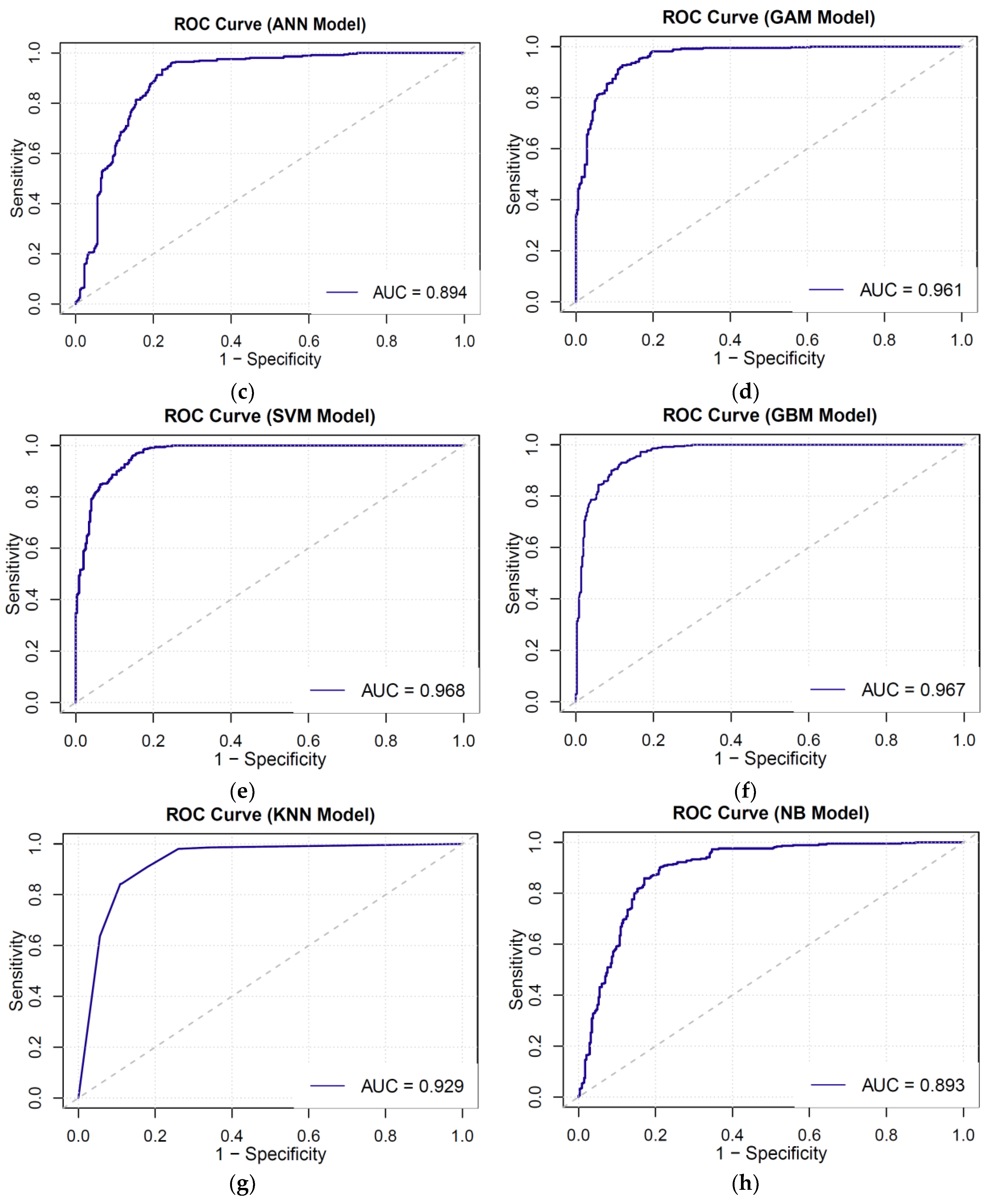
Area under the ROC curve (AUC-ROC): The ROC curve is a graphical representation of the true-positive rate plotted against the false-positive rate. It illustrates the balance between sensitivity and specificity. AUC-ROC serves as a metric indicating the effectiveness of a parameter in discriminating between two diagnostic groups (diseased/normal). A higher AUC value corresponds to a superior ability of the model to distinguish between trees that perished and those that endured.
These metrics were calculated for each model using the ‘pROC’ and ‘caret’ packages in R. The models were then compared based on these metrics to determine the best performing model.

3. Results

3.1. Model Fitting Accuracy

Using the SMOTE method, 1185 dead trees’ data were produced. Based on the dataset of 1222 living trees and 1185 dead trees, the modeling work was carried out. The distribution of DBH based on mortality status after oversampling is available in the supplementary materials, depicted in Figure S2. In this study, we evaluated eight distinct machine learning models to understand their fitting accuracy to the training dataset. The detailed evaluation of each model is as follows and is also shown in Table 2.
The RF model exhibits exceptional performance, marked by near-perfect precision (99.76%) and very high levels of accuracy (97.93%), sensitivity (96.23%), and an F1 score (97.96%), underscoring its superior predictive capability and reliability in accurately classifying tree mortality. Its high Kappa value (0.9585) further indicates a significant agreement beyond chance, making it a robust choice for complex ecological predictions.

3.2. Model Prediction Accuracy Evaluation on Test Dataset

The performance of the eight machine learning models was further validated on the test dataset. The evaluation metrics for each model are detailed below and are also shown in Table 3:
The prediction statistics of the eight machine learning models on the test dataset are analyzed, focusing on the relative performance and effectiveness of each model across various metrics such as accuracy, sensitivity, specificity, Kappa, precision, and F1 score. Based on the results of the model performance metrics, it can be observed that the random forest (RF) model excels, demonstrating the highest accuracy (0.9291) and a Kappa statistic of 0.8580. It achieves commendable scores in both sensitivity (0.9277) and specificity (0.9303). The naive Bayes (NB) model exhibits worst performance compared to random forest, with accuracy and Kappa statistics reaching the same levels (0.8391 and 0.6773, respectively). Other models, such as logistic regression (LR), artificial neural network (ANN), generalized additive model (GAM), support vector machine (SVM), gradient boosting machine (GBM), and k-nearest neighbors (K-NN), also perform well, albeit with slight variations in certain metrics.

3.3. AUC-ROC Curve

The ROC curves were constructed, and the area under the curve (AUC) was computed to quantify the discriminative ability of the models (Figure 2). The RF model exhibited an AUC of 0.966, indicating a very high level of discriminative capacity. The LR model followed with an AUC of 0.898, and the ANN model presented an AUC of 0.894, showing substantial predictive power. The GAM demonstrated robust discrimination with an AUC of 0.961, whereas the SVM model achieved an AUC of 0.968, slightly surpassing the GAM. The GBM model also showed excellent performance with an AUC of 0.967, closely matching the SVM model. The K-NN model yielded an AUC of 0.929, indicating good classification ability, while the NB model had an AUC of 0.893, which, despite being the lowest in this group, still represents a good discriminative ability.

3.4. Variables Importance

In this study, we employed eight distinct machine learning models to analyze and predict the target variable. These models encompass the ANN, GAM, LR, RF, GBM, KNN, NB and SVM models. The results are shown in Figure 3.
The random forest model, prioritized BAL, DBH, BA, elevation, slope, NH4-N, moisture, CD, and available P. The consistent emphasis on BAL and DBH across most models, coupled with the varied importance of factors like elevation, slope, and soil nutrients such as NH4-N and the available P, demonstrates the intricate interplay of physical and environmental variables in tree ecology. Through the analysis of eight different machine learning models, the BAL, DBH, and BA variables were found to be of high importance in most models. Additionally, other variables such as crown density, elevation, slope, and the available P and NH4-N also exhibited high levels of importance in certain models.

4. Discussion

Based on the performance metrics derived from both the training and test datasets, we observe nuanced insights into the predictive capabilities of the eight machine learning models employed in our study on tree mortality. The RF model showcased the best performance, with the highest precision and the highest accuracy, underscoring its robustness across various metrics. This model also demonstrated a high Kappa score, indicating a strong agreement beyond chance in its predictions, making it the most reliable model for predicting outcomes accurately.
In contrast, the LR and NB models showed foundational performance with reasonable metrics, indicating that they may struggle with complex data relationships compared to more sophisticated models. However, GBM exhibited superior performance, particularly in accuracy, and it had the highest F1 score, highlighting its capability in handling variable interactions and non-linear dynamics effectively. The SVM model also performed well, demonstrating high levels of accuracy and precision, suggesting it is effective in minimizing false positives. The K-NN model, while not achieving the highest scores, still provided a solid performance across all metrics, particularly in terms of its AUC-ROC curve, which suggests good classification ability.
In conclusion, the analysis underscores the RF and GBM models as the most promising in terms of accuracy, reliability, and overall performance. These models strike an excellent balance between precision and sensitivity, adeptly predicting outcomes most of the time. However, model selection should still consider specific project requirements, including computational costs and the implications of various types of prediction errors. Conversely, models like NB and LR, while offering solid foundational capabilities, display limitations in their predictive performance, likely due to their simpler nature and assumptions, which may not capture the intricate relationships within the data effectively.
The pivotal role of BAL as the most significant variable in predicting individual tree mortality underscores the intricate dynamics of forest stand structure and competition within ecosystems. This finding is consistent with ecological theories and empirical evidence suggesting that the spatial distribution and size hierarchy within a forest significantly affect individual tree growth, survival, and overall forest productivity [70].
The prominence of BAL within our analysis underscores the principle of competitive exclusion, illustrating that the trees within more densely populated stands surrounded by trees with greater basal areas, are at an increased risk of experiencing stunted growth and a higher likelihood of mortality. This struggle for vital resources like sunlight, water, and minerals intensifies when the basal area of neighboring trees surpasses that of the focal tree, resulting in increased stress and a potential rise in mortality. Essentially, trees that boast a larger basal area are better positioned to monopolize these resources, overshadowing their smaller counterparts and outperforming them for access to water and soil nutrients.
DBH is indicative of tree size, age, growth rate, and resilience [8] and is largely included as variable in tree mortality research [71,72,73] and emerged as a pivotal variable across several models with notable importance values such as 1.0000 in GAM, around 0.7 in the RF, SVM, KNN, and NB models. The prominence of DBH aligns with the understanding that trees with larger diameters are typically more resilient to environmental stressors [74]. However, the models also allude to intricate interactions, implying that specific conditions may challenge even trees with substantial DBH.
The mortality caused by competition for light, water, temperature, and nutrients is referred to as intrinsic mortality. Intrinsic mortality is influenced over the long term by the genetic and physiological characteristics of tree species, site conditions, and climatic factors [75]. Site conditions form the foundation of forest productivity and are closely tied to tree mortality. The present study primarily incorporates topography-related factors as site variables, encompassing elevation, aspect, position on slope, gradient, and microtopography. These factors predominantly influence hydrothermal factors and soil conditions directly associated with tree growth [76]. In this study, we applied slope and elevation as factors. Elevation, a factor influencing temperature, humidity, light, and soil characteristics, was accentuated in various models, particularly in the ANN model. This finding resonates with the ecological theories that particular altitudes may predispose certain tree species to mortality, underscoring the complex equilibrium between environmental parameters and tree vitality. In mountainous regions characterized by significant variations in elevation, distinct vegetation-vertical-zonation profiles are formed due to the undulating topography [77]. Slope, a determinant of soil erosion, moisture retention, and light exposure, was emphasized in models such as ANN, KNN and RF. While its ecological relevance in shaping tree growth and survival is recognized, slope was not uniformly significant across all models. This discrepancy invites further exploration to elucidate slope’s multifaceted role in forest ecology. Li Chunming et al. [78] also attempted to incorporate the influencing factors of aspect and elevation in their study on stand mortality in Mongolian oak forests. However, they found that the model outcomes indicated that these independent variables did not qualify for inclusion in the model. This result is different from our result. We attributed this outcome to the relatively low elevation (600–750 m) in their research and the high elevation (2079–2438 m) in our research.
CD, a measure of forest canopy cover, was highlighted in models like RF, SVM, KNN and NB. Within a given species, superior tree health is commonly linked to higher crown density values, reduced foliage transparency values, and diminished crown dieback values [79]. The models’ focus on CD reflects its critical influence on sunlight penetration, photosynthesis efficiency, and overall tree growth, emphasizing the intricate relationship between canopy architecture and arboreal survival.
Soil plays a pivotal role in tree growth by providing essential nutrients, moisture, and structural support. Among the spectrum of soil nutrients, NH4-N and available P, assume a critical role in tree physiological processes. The soil’s NH4-N content significantly influences plant health and growth by modifying nitrogen absorption efficiency, altering soil pH, and impacting the root environment’s microbial ecosystem. Too much NH4-N can cause nitrogen toxicity, negatively affecting plant growth, while too little may hinder plant development and reduce productivity [80].
Phosphorus, being a fundamental constituent of ATP, nucleic acids, and phospholipids, exerts profound influence on tree development and growth when present in the form of available P [81]. In forest ecosystems, the concentration of available P within the soil can emerge as a constraining factor, especially within regions characterized by weathered or phosphorus-depleted soils [82]. The association between available P and tree vitality is intricate and multifaceted, often interacting with various other soil attributes and environmental variables. Grasping this relationship holds paramount importance in forest management and conservation, as it underscores the intricate equilibrium between soil fertility and tree well-being. The available P, denoting the available phosphorus in the soil, was underscored in models such as RF and ANN. As an essential nutrient for plant growth, the importance of the available P in these models suggests that phosphorus scarcity may constrain tree development. Although not uniformly significant, its ecological relevance merits further investigation.
In conclusion, these patterns of variable importance furnish invaluable insights into the mechanisms governing tree mortality, unveiling the synergistic interactions between tree attributes, soil nutrients, topographical variations, and tree mortality. The disparities in variable importance across models illuminate the unique attributes and sensitivities of each modeling approach, providing a road map for model selection tailored to specific ecological inquiries and management goals. This comprehensive assessment augments our understanding of individual tree characteristics and accentuates the significance of judicious model selection and feature engineering in advancing ecological research.
This study integrates machine learning insights with ecological theories and offers a multifaceted perspective on tree mortality factors. The prominence of variables such as BAL, BA, DBH, elevation, and CD across different models underscores their importance, while also highlighting the need for a nuanced understanding of other variables like slope, available P, and NH4-N. Future research should consider these complex interactions and the specific context of tree species, location, and environmental conditions.
Additionally, our study has some limitations. Firstly, our dataset may have biases as it comes from specific populations and regions. Secondly, the models might be influenced by the lack of data on dead trees or further influenced by data pre-processing methods. Future research can further improve model performance by using more diverse datasets and exploring different feature engineering techniques.

5. Conclusions

In this study, eight diverse machine learning methods were harnessed to formulate a predictive model for individual tree mortality. Our analysis revealed varying performance across methodologies; random forest demonstrated the best prediction performance. The significance of tree- and stand-level factors, and site and soil factors, in predicting tree mortality was emphasized, underscoring the necessity of encompassing these multifaceted elements within the model.
Notably, the variables significantly impacting individual tree mortality were identified through feature importance analysis across models: BAL, DBH, BA, elevation, slope, NH4-N, soil moisture, crown density, and the soil’s available phosphorus are important variables in the Larix gmelinii var. principis-rupprechtii individual mortality model. This emphasizes the role of the tree growth environment, physiological traits, and soil phosphorus content. Although promising, challenges including data limitations and ecosystem complexity should be considered when applying the model. This study exemplifies the potential of machine learning for predicting tree mortality, offering insights for model enhancement, and aiding ecosystem-management decisions.

Supplementary Materials

The following supporting information can be downloaded at: https://www.mdpi.com/article/10.3390/f15020374/s1, Figure S1: Original Distribution of tree DBH by mortality status, Figure S2: Distribution of tree DBH by mortality status.

Author Contributions

Formal analysis, Z.Y., G.D. and R.P.S.; methodology, G.D.; software, G.D., W.P. and Y.F.; supervision, R.P.S. and M.Z.; validation, M.Z.; visualization, Z.Y.; writing—original draft, Z.Y., G.D., W.P., L.Z. and Y.F.; writing—review and editing, R.P.S. and M.Z. All authors have read and agreed to the published version of the manuscript.

Funding

This research was funded by the following projects: Shanxi Province Basic Research Program, Youth Science Research Project: NO. 202203021212425; Shanxi Province Key Research and Development Program: 202102090301007; National Natural Science Foundation of China: 31901308.

Data Availability Statement

The data that support the findings of this study are available from the Research Institute of Forest Resource Information Techniques, the Chinese Academy of Forestry. Restrictions apply to the availability of these data, which were used under license for this study. Data are available from the authors with the permission of the Research Institute of Forest Resource Information Techniques, the Chinese Academy of Forestry.

Acknowledgments

We thank the Research Institute of Forest Resource Information Techniques, the Chinese Academy of Forestry for data support. We are thankful to three anonymous reviewers for their constructive comments and recommendations, which helped improve the article.

Conflicts of Interest

The authors declare that they have no conflicts of interest.

References

  1. FAO. Global Ecological Zoning for the Global Forest Resources Assessment Key Findings; FAO: Rome, Italy, 2020. [Google Scholar]
  2. Millar, C.I.; Stephenson, N.L. Temperate forest health in an era of emerging megadisturbance. Science 2015, 349, 823–826. [Google Scholar] [CrossRef]
  3. Nowak, D.J.; Crane, D.E.; Stevens, J.C.; Hoehn, R.E.; Walton, J.T.; Bond, J. A ground-based method of assessing urban forest structure and ecosystem services. Arboric. Urban. For. 2008, 34, 347–358. [Google Scholar] [CrossRef]
  4. Breshears, D.D.; Cobb, N.S.; Rich, P.M.; Price, K.P.; Allen, C.D.; Balice, R.G.; Romme, W.H.; Kastens, J.H.; Floyd, M.L.; Belnap, J.; et al. Regional vegetation die-off in response to global-change-type drought. Proc. Natl. Acad. Sci. USA 2005, 102, 15144–15148. [Google Scholar] [CrossRef]
  5. Hawkes, C. Woody plant mortality algorithms: Description, problems and progress. Ecol. Modell. 2000, 126, 225–248. [Google Scholar] [CrossRef]
  6. Searle, E.B.; Chen, H.Y.; Paquette, A. Higher tree diversity is linked to higher tree mortality. Proc. Natl. Acad. Sci. USA 2022, 119, e2013171119. [Google Scholar] [CrossRef]
  7. Rita, A.; Borghetti, M. Linkage of forest productivity to tree diversity under two different bioclimatic regimes in Italy. Sci. Total Environ. 2019, 687, 1065–1072. [Google Scholar] [CrossRef] [PubMed]
  8. Zhang, X.-Q.; Lei, Y.-C.; Liu, X.-Z. Modeling stand mortality using Poisson mixture models with mixed-effects. iForest 2014, 8, 333–338. [Google Scholar] [CrossRef]
  9. Ruiz-Benito, P.; Ratcliffe, S.; Zavala, M.A.; Martínez-Vilalta, J.; Vilà-Cabrera, A.; Lloret, F.; Madrigal-González, J.; Wirth, C.; Greenwood, S.; Kändler, G.; et al. Climate- and successional-related changes in functional composition of European forests are strongly driven by tree mortality. Glob. Chang. Biol. 2017, 23, 4162–4176. [Google Scholar] [CrossRef] [PubMed]
  10. Muscarella, R.; Lohbeck, M.; Martínez-Ramos, M.; Poorter, L.; Rodríguez-Velázquez, J.E.; van Breugel, M.; Bongers, F. Demographic drivers of functional composition dynamics. Ecology 2017, 98, 2743–2750. [Google Scholar] [CrossRef] [PubMed]
  11. Larson, A.J.; Lutz, J.A.; Donato, D.C.; Freund, J.A.; Swanson, M.E.; HilleRisLambers, J.; Sprugel, D.G.; Franklin, J.F. Spatial aspects of tree mortality strongly differ between young and old-growth forests. Ecology 2015, 96, 2855–2861. [Google Scholar] [CrossRef]
  12. Thom, D.; Seidl, R. Natural disturbance impacts on ecosystem services and biodiversity in temperate and boreal forests. Biol. Rev. 2016, 91, 760–781. [Google Scholar] [CrossRef]
  13. Bugmann, H.; Seidl, R.; Hartig, F.; Bohn, F.; Brůna, J.; Cailleret, M.; François, L.; Heinke, J.; Henrot, A.; Hickler, T.; et al. Tree mortality submodels drive simulated long-term forest dynamics: Assessing 15 models from the stand to global scale. Ecosphere 2019, 10, e02616. [Google Scholar] [CrossRef] [PubMed]
  14. Korner, C. A matter of tree longevity. Science 2017, 355, 130–131. [Google Scholar] [CrossRef] [PubMed]
  15. Mayer, M.; Sandén, H.; Rewald, B.; Godbold, D.L.; Katzensteiner, K. Increase in heterotrophic soil respiration by temperature drives decline in soil organic carbon stocks after forest windthrow in a mountainous ecosystem. Funct. Ecol. 2017, 31, 1163–1172. [Google Scholar] [CrossRef]
  16. Weng, Z.; Van Zwieten, L.; Singh, B.P.; Tavakkoli, E.; Joseph, S.; Macdonald, L.M.; Rose, T.J.; Rose, M.T.; Kimber, S.W.L.; Morris, S.; et al. Biochar built soil carbon over a decade by stabilizing rhizodeposits. Nat. Clim. Chang. 2017, 7, 371–376. [Google Scholar] [CrossRef]
  17. Thorn, S.; Seibold, S.; Leverkus, A.B.; Michler, T.; Müller, J.; Noss, R.F.; Stork, N.; Vogel, S.; Lindenmayer, D.B. The living dead: Acknowledging life after tree death to stop forest degradation. Front. Ecol. Environ. 2020, 18, 505–512. [Google Scholar] [CrossRef]
  18. Liu, Q.; Peng, C.; Schneider, R.; Cyr, D.; McDowell, N.G.; Kneeshaw, D. Drought-induced increase in tree mortality and corresponding decrease in the carbon sink capacity of Canada’s boreal forests from 1970 to 2020. Glob. Chang. Biol. 2023, 29, 2274–2285. [Google Scholar] [CrossRef]
  19. Lewis, S.L.; Phillips, O.L.; Sheil, D.; Vinceti, B.; Baker, T.R.; Brown, S.; Graham, A.W.; Higuchi, N.; Hilbert, D.W.; Laurance, W.F.; et al. Tropical forest tree mortality, recruitment and turnover rates: Calculation, interpretation and comparison when census intervals vary. J. Ecol. 2004, 92, 929–944. [Google Scholar] [CrossRef]
  20. Hember, R.A.; Kurz, W.A.; Coops, N.C. Relationships between individual-tree mortality and water-balance variables indicate positive trends in water stress-induced tree mortality across North America. Glob. Chang. Biol. 2017, 23, 1691–1710. [Google Scholar] [CrossRef]
  21. Fortin, M.; Bédard, S.; DeBlois, J.; Meunier, S. Predicting individual tree mortality in northern hardwood stands under uneven-aged management in southern Québec, Canada. Ann. For. Sci. 2008, 65, 205. [Google Scholar] [CrossRef]
  22. Temesgen, H.; Mitchell, S.J. An individual-tree mortality model for complex stands of southeastern British Columbia. West. J. Appl. For. 2005, 20, 101–109. [Google Scholar] [CrossRef]
  23. Dobbertin, M.; Biging, G.S. Using the non-parametric classifier CART to model forest tree mortality. For. Sci. 1998, 44, 507–516. [Google Scholar]
  24. Clark, P.; Wyckoff, J. Predicting tree mortality from diameter growth: A comparison of maximum likelihood and Bayesian approaches. Can. J. For. Res. 2000, 30, 156–167. [Google Scholar] [CrossRef]
  25. Affleck, D.L.R. Poisson mixture models for regression analysis of stand-level mortality. Can. J. For. Res. 2006, 36, 2994–3006. [Google Scholar] [CrossRef]
  26. Vieilledent, G.; Courbaud, B.; Kunstler, G.; Dhôte, J.-F.; Clark, J.S. BBiases in the estimation of size-dependent mortality models: Advantages of a semiparametric approach. Can. J. For. Res. 2009, 39, 1430–1443. [Google Scholar] [CrossRef]
  27. Adame, P.; Del Río, M.; Cañellas, I. Modeling individual-tree mortality in Pyrenean oak (Quercus pyrenaica Willd. ) stands. Ann. For. Sci. 2010, 67, 810. [Google Scholar] [CrossRef]
  28. Neumann, M.; Mues, V.; Moreno, A.; Hasenauer, H.; Seidl, R. Climate variability drives recent tree mortality in Europe. Glob. Chang. Biol. 2017, 23, 4788–4797. [Google Scholar] [CrossRef]
  29. Vanclay J, K. Modelling Forest Growth and Yield: Applications Tomixed and Tropical Forests; CAB International: Wallingford, UK, 1994. [Google Scholar]
  30. Han, P. Climate-Sensitive Growth and Mortality Model of Changbai Larch (Larix olgensis) Forests. Ph.D. Thesis, Beijing Forestry University, Beijing, China, 2020. (In Chinese). [Google Scholar]
  31. Ferry, B.; Morneau, F.; Bontemps, J.D.; Blanc, L.; Freycon, V. Higher treefall rates on slopes and waterlogged soils result in lower stand biomass and productivity in a tropical rain forest. J. Ecol. 2010, 98, 106–116. [Google Scholar] [CrossRef]
  32. Kuster, T.; Arend, M.; Bleuler, P.; Günthardt-Goerg, M.S.; Schulin, R. Water regime and growth of young oak stands subjected to air-warming and drought on two different forest soils in a model ecosystem experiment. Plant Biol. 2013, 15, 138–147. [Google Scholar] [CrossRef]
  33. Arend, M.; Gessler, A.; Schaub, M. The influence of the soil on spring and autumn phenology in European beech. Tree Physiol. 2016, 36, 78–85. [Google Scholar] [CrossRef]
  34. Buchman, R.; Pederson, S.; Walters, N. A tree survival model with application to species of the Great Lakes region. Can. J. For. Res. 1983, 13, 601–608. [Google Scholar] [CrossRef]
  35. Brang, D. Crown defoliation improves tree mortality models. For. Ecol. Manag. 2001, 141, 271–284. [Google Scholar]
  36. Zhao, D.; Borders, B.; Wilson, M. Individual-tree diameter growth and mortality models for bottomland mixed-species hardwood stands in the lower Mississippi alluvial valley. For. Ecol. Manag. 2004, 199, 307–322. [Google Scholar] [CrossRef]
  37. Coyea, M.; Margolis, H. The historical reconstruction of growth efficiency and its relationship to tree mortality in balsam fir ecosystems affected by spruce budworm. Can. J. For. Res. 1994, 24, 2208–2221. [Google Scholar] [CrossRef]
  38. Crecente-Campo, F.; Marshall, P.; Rodríguez-Soalleiro, R. Modeling non-catastrophic individual-tree mortality for Pinus radiata plantations in northwestern Spain. For. Ecol. Manag. 2009, 257, 1542–1550. [Google Scholar] [CrossRef]
  39. Holzwarth, F.; Kahl, A.; Bauhus, J.; Wirth, C. Many ways to die–partitioning tree mortality dynamics in a near-natural mixed deciduous forest. J. Ecol. 2013, 101, 220–230. [Google Scholar] [CrossRef]
  40. Peng, C.; Ma, Z.; Lei, X.; Zhu, Q.; Chen, H.; Wang, W.; Liu, S.; Li, W.; Fang, X.; Zhou, X. A drought-induced pervasive increase in tree mortality across Canada’s boreal forests. Nat. Clim. Chang. 2011, 1, 467–471. [Google Scholar] [CrossRef]
  41. Zhu, K.; Ran, Y.; Ma, M.; Li, W.; Mir, Y.; Ran, J.; Wu, S.; Huang, P. Ameliorating soil structure for the reservoir riparian: The influences of land use and dam-triggered flooding on soil aggregates. Soil. Tillage Res. 2020, 216, 105263. [Google Scholar] [CrossRef]
  42. Mao, Q.; Lu, X.; Wang, C.; Zhou, K.; Mo, J. Responses of understory plant physiological traits to a decade of nitrogen addition in a tropical reforested ecosystem. For. Ecol. Manag. 2017, 401, 65–74. [Google Scholar] [CrossRef]
  43. Bu, W.-S.; Chen, F.-S.; Wang, F.-C.; Fang, X.-M.; Mao, R.; Wang, H.-M. The species-specific responses of nutrient resorption and carbohydrate accumulation in leaves and roots to nitrogen addition in a subtropical mixed plantation. Can. J. For. Res. 2019, 49, 826–835. [Google Scholar] [CrossRef]
  44. Sarkar, D.; Bali, R.; Sharma, T. Machine Learning Basics. In Practical Machine Learning with Python; Springer: Apress, Berkeley, CA, 2018. [Google Scholar] [CrossRef]
  45. Wang, J.; Taylor, A.R.; D’Orangeville, L. Warming-induced tree growth may help offset increasing disturbance across the Canadian boreal forest. Proc. Natl. Acad. Sci. USA 2023, 120, e2212780120. [Google Scholar] [CrossRef]
  46. Alenius, V.; Hökkä, H.; Salminen, H.; Jutras, S. Evaluating estimation methods for logistic regression in modelling individual-tree mortality. In Modelling Forest Systems; CABI Publishing: Wallingford, UK, 2003; pp. 225–236. [Google Scholar]
  47. Thomas, F.; Petzold, R.; Becker, C.; Werban, U. Usage of visual and near-infrared spectroscopy to predict soil properties in forest stands. In Proceedings of the EGU General, Assembly Conference Abstracts, Online, 4–8 May 2020; p. 9107. [Google Scholar]
  48. Wang, Z.; Zhang, X.; Chhin, S.; Zhang, J.; Duan, A. Disentangling the effects of stand and climatic variables on forest productivity of Chinese fir plantations in subtropical China using a random forest algorithm. Agric. For. Meteorol. 2021, 304, 108412. [Google Scholar] [CrossRef]
  49. Lou, X.W.; Weng, Y.H.; Fang, L.M.; Gao, H.L.; Grogan, J.; Hung, I.K.; Oswald, B.P. Predicting stand attributes of loblolly pine in West Gulf Coastal Plain using gradient boosting and random forests. Can. J. For. Res. 2021, 51, 807–816. [Google Scholar] [CrossRef]
  50. Walia, N.K.; Kalra, P.; Mehrotra, D. Prediction of carbon stock available in forest using naive Bayes approach. In Proceedings of the 2016 Second International Conference on Computational Intelligence & Communication Technology (CICT), Ghaziabad, India, 12–13 February 2016; pp. 275–279. [Google Scholar] [CrossRef]
  51. Fu, L.; Zhang, H.; Sharma, R.P.; Pang, L.; Wang, G. A generalized nonlinear mixed-effects height to crown base model for Mongolian oak in northeast China. For. Ecol. Manag. 2017, 384, 34–43. [Google Scholar] [CrossRef]
  52. Rozas, V. Tree age estimates in Fagus sylvatica and Quercus robur: Testing previous and improved methods. Plant Ecol. 2003, 167, 193–212. [Google Scholar] [CrossRef]
  53. Du, J.S.; Wang, H.L.; Tang, S.Z. Update models of forest resource data for subcompartments in natural forest. Sci. Silvae Sin. 2000, 36, 26–32. [Google Scholar]
  54. Chawla, N.V.; Bowyer, K.W.; Hall, L.O.; Kegelmeyer, W.P. SMOTE: Synthetic minority over-sampling technique. J. Artif. Intell. Res. 2002, 16, 321–357. [Google Scholar] [CrossRef]
  55. R Core Team. R: A Language and Environment for Statistical Computing; R Foundation for Statistical Computing: Vienna, Austria, 2018; Available online: https://www.R-project.org/ (accessed on 1 June 2023).
  56. Cutler, D.R.; Edwards, T.C., Jr.; Beard, K.H.; Cutler, A.; Hess, K.T.; Gibson, J.; Lawler, J.J. Random forests for classification in ecology. Ecology 2007, 88, 2783–2792. [Google Scholar] [CrossRef]
  57. McRoberts, R.E.; Næsset, E.; Gobakken, T. Optimizing the k-Nearest Neighbors technique for estimating forest aboveground biomass using airborne laser scanning data. Remote Sens. Environ. 2015, 163, 13–22. [Google Scholar] [CrossRef]
  58. King, S.L.; Bennett, K.P.; List, S. Modeling noncatastrophic individual tree mortality using logistic regression, neural networks, and support vector methods. Comput. Electron. Agric. 2000, 27, 401–406. [Google Scholar] [CrossRef]
  59. Hasenauer, H.; Merkl, D.; Weingartner, M. Estimating tree mortality of Norway spruce stands with neural networks. Adv. Environ. Res. 2001, 5, 405–414. [Google Scholar] [CrossRef]
  60. Castro, R.V.O.; Soares, C.P.B.; Leite, H.G.; de Souza, A.L.; Nogueira, G.S.; Martins, F.B. Individual growth model for Eucalyptus stands in Brazil using artificial neural network. ISRN For. 2013, 196832. [Google Scholar] [CrossRef]
  61. Reis, L.P.; de Souza, A.L.; dos Reis, P.C.M.; Mazzei, L.; Soares, C.P.B.; Torres, C.M.M.E.; da Silva, L.F.; Ruschel, A.R.; Rêgo, L.J.S.; Leite, H.G. Estimation of mortality and survival of individual trees after harvesting wood using artificial neural networks in the amazon rain forest. Ecol. Eng. 2018, 112, 140–147. [Google Scholar] [CrossRef]
  62. Breiman, L. Random Forests. Mach. Learn. 2001, 45, 5–32. [Google Scholar] [CrossRef]
  63. Cox, D.R. The regression analysis of binary sequences. J. R. Stat. Soc. Ser. B Stat. Methodol. 1958, 20, 215–232. [Google Scholar] [CrossRef]
  64. Artin, N.; Chung, K.L. Theory of Probability and its Applications. Vol. III—1958. In An English Translation of the Soviet Journal Teoriya Veroyatnosteĭ i ee Primeneniya; Geological Society Publishing House: Bath, UK, 1990. [Google Scholar]
  65. Hastie, T.J.; Tibshirani, R.J. Generalized Additive Models. Stat. Sci. 1986, 1, 297–318. [Google Scholar] [CrossRef]
  66. Zhang, Z. Introduction to machine learning: K-nearest neighbors. Ann. Transl. Med. 2016, 4, 218. [Google Scholar] [CrossRef] [PubMed]
  67. Rish, I. An empirical study of the naive Bayes classifier. In Proceedings of the IJCAI 2001 Workshop on Empirical Methods in Artificial Intelligence, Seattle, WA, USA, 4–6 August 2001; Volume 4, pp. 41–46. [Google Scholar]
  68. Friedman, J.H. Greedy function approximation: A gradient boosting machine. Ann. Stat. 2001, 1, 1189–1232. [Google Scholar] [CrossRef]
  69. Krenker, A.; Bešter, J.; Kos, A. Introduction to the artificial neural networks. In Artificial Neural Networks: Methodological Advances and Biomedical Applications; InTech: London, UK, 2011; pp. 1–18. [Google Scholar]
  70. Hamidi, S.K.; Zenner, E.K.; Bayat, M.; Fallah, A. Analysis of plot-level volume increment models developed from machine learning methods applied to an uneven-aged mixed forest. Ann. For. Sci. 2021, 78, 4. [Google Scholar] [CrossRef]
  71. Zhou, X.; Chen, Q.; Sharma, R.P.; Wang, Y.; He, P.; Guo, J.; Lei, Y.; Fu, L. A climate sensitive mixed-effects diameter class mortality model for Prince Rupprecht larch (Larix gmelinii var. principis-rupprechtii) in northern China. For. Ecol. Manag. 2021, 491, 119091. [Google Scholar] [CrossRef]
  72. Zhou, X.; Fu, L.; Sharma, R.P.; He, P.; Lei, Y.; Guo, J. Generalized or general mixed-effect modelling of tree mortality of Larix gmelinii subsp. principis-rupprechtii in Northern China. J. For. Res. 2021, 32, 2447–2458. [Google Scholar] [CrossRef]
  73. Xie, L.; Chen, X.; Zhou, X.; Sharma, R.P.; Li, J. Developing tree mortality models using bayesian modeling approach. Forests 2022, 13, 604. [Google Scholar] [CrossRef]
  74. Yao, X.; Titus, S.J.; Macdonald, S.E. A generalized logistic model of individual tree mortality for aspen, white spruce, and lodgepole pine in Alberta mixedwood forests. Can. J. For. Res. 2001, 31, 283–291. [Google Scholar] [CrossRef]
  75. Lutz, J.A.; Halpern, C.B. Tree mortality during early forest development: A long-term study of rates causes, and consequences. Ecol. Monogr. 2006, 76, 257–275. [Google Scholar] [CrossRef]
  76. Bałazy, R.; Kamińska, A.; Ciesielski, M.; Socha, J.; Pierzchalski, M. Modeling the effect of environmental and topographic variables affecting the height increment of Norway spruce stands in mountainous conditions with the use of LiDAR data. Remote Sens. 2019, 11, 2407. [Google Scholar] [CrossRef]
  77. Stage, A.R.; Christian, S. Interactions of Elevation, Aspect, and Slope in Models of Forest Species Composition and Productivity. For. Sci. 2007, 53, 486–492. [Google Scholar]
  78. Li, C.; Zhao, L.; Li, L. Modeling stand-Level mortality of Mongolian Oak (Quercus mongolica) based on mixed effect model and zero-inflated model methods. For. Sci. 2019, 55, 27–36. (In Chinese) [Google Scholar]
  79. Morin, R.S.; Randolph, K.C.; Steinman, J. Mortality rates associated with crown health for eastern forest tree species. Environ. Monit. Assess. 2015, 187, 87. [Google Scholar] [CrossRef]
  80. Zhu, Y.; Qi, B.; Hao, Y.S.; Liu, H.; Sun, G.; Chen, R.; Song, S. Appropriate NH4+/NO3 ratio triggers plant growth and nutrient uptake of flowering Chinese cabbage by optimizing the pH value of nutrient solution. Front. Plant Sci. 2021, 12, 656144. [Google Scholar] [CrossRef]
  81. Richardson, A.E.; Lynch, J.P.; Ryan, P.R.; Delhaize, E.; Smith, F.A.; Smith, S.E.; Harvey, P.R.; Ryan, M.H.; Veneklaas, E.J.; Lambers, H.; et al. Plant and microbial strategies to improve the phosphorus efficiency of agriculture. Plant Soil. 2011, 349, 121–156. [Google Scholar] [CrossRef]
  82. Vitousek, P.M.; Porder, S.; Houlton, B.Z.; Chadwick, O.A. Terrestrial phosphorus limitation: Mechanisms, implications, and nitrogen–phosphorus interactions. Ecol. Appl. 2010, 20, 5–15. [Google Scholar] [CrossRef] [PubMed]
Figure 1. Study area with sample plots’ location (dots represent sample plot positions).
Forests 15 00374 g001
Figure 2. AUC–ROC curve across models. (a) RF model ROC curve; (b) LR model ROC curve; (c) ANN model ROC curve; (d) GAM model ROC curve; (e) SVM model ROC curve; (f) GBM model ROC curve; (g) KNN model ROC curve; (h) NB model ROC curve. (The grey dotted line is a diagonal line representing the predictive performance of a random guessing model).
Forests 15 00374 g002aForests 15 00374 g002b
Figure 3. Variables’ importance across models: (a), ANN model; (b), GAM model; (c), LR model; (d), RF model; (e), GBM model; (f), KNN model; (g), NB model; (h) SVM model.
Forests 15 00374 g003
Table 1. Summary statistics of measurements for individual, stand-level variables and soil characters variables.
VariableMinMaxMeanStd
DBH (cm)0.90 44.5013.1910 8.7541
BA (cm2)0.641554.50196.6600226.2700
BAL (cm2)0.0019,543.619698.37004396.1000
Thickness (cm)1.80 12.00 5.8732 2.8754
CD0.54 0.92 0.7678 0.1200
Elevation (m)2079 2438 2239 97.4420
DA26.00 71.00 53.0115 14.3212
Slope (degree)8.00 38.50 22.9313 6.8836
Moisture (%)12.38 37.46 26.0389 6.5818
Density (g/m3)0.72 1.71 1.0107 0.2129
PH6.40 6.776.6103 0.1012
TC (g/kg)1.29 4.25 2.5476 0.8757
NO3-N (mg/kg)6.81 18.98 10.5527 3.7009
NH4-N (mg/kg)9.92 64.67 21.6761 10.9171
Available K (mg/kg)48.35 90.62 65.9163 9.4617
Available P (mg/kg)3.31 10.88 5.5186 1.9669
Age16 70 39.7297 16.4208
Note: DBH: diameter at breast height, BA: basal area; BAL: basal area larger than the target trees; Thickness: soil thickness; CD: crown density; Elevation: the elevation at which the trees are located; DA: average age of dominant trees; Slope: slope degree; Moisture: water content of soil; Density: The ratio of the mass of a certain volume of soil after drying to the volume before drying; PH: the PH value of soil; TC: total carbon content of soil; NO3-N: nitrate nitrogen; NH4-N: ammonium nitrogen; Available K: available potassium content of soil; Available P: available phosphorus content of soil; Age: average age of the average trees in a certain plot.
Table 2. Fitting statistics of the eight models on fitting dataset.
ModelAccuracySensitivitySpecificityKappaPrecisionF1 Score
RF0.97930.96230.99750.95850.99760.9796
LR0.84880.80390.89690.69840.89300.8461
ANN0.86600.81790.91760.73260.91420.8634
GAM0.89460.85100.93550.78840.92520.8866
SVM0.90280.86810.93990.80590.93920.9023
GBM0.94550.93390.95760.89090.95830.9459
K-NN0.90520.86010.95260.81070.95020.9029
NB0.83990.79790.88520.68050.88260.8381
Table 3. Prediction statistics of the eight models for test dataset.
ModelAccuracySensitivitySpecificityKappaPrecisionF1 Score
RF0.92910.92770.93030.85800.92510.9259
LR0.84720.81430.87840.69370.86360.8386
ANN0.85990.79080.92470.71840.90790.8459
GAM0.89460.85100.93550.78840.92520.8867
SVM0.89720.86570.92700.79400.91820.8916
GBM0.90420.88610.92220.80830.91930.9033
K-NN0.86530.82070.90910.73030.89880.8588
NB0.83910.81500.86130.67730.84430.8294
Disclaimer/Publisher’s Note: The statements, opinions and data contained in all publications are solely those of the individual author(s) and contributor(s) and not of MDPI and/or the editor(s). MDPI and/or the editor(s) disclaim responsibility for any injury to people or property resulting from any ideas, methods, instructions or products referred to in the content.

