1. Introduction
Digital Twins (DT) are virtual representations of real-world objects [
1]. Digital twins can enhance the performance of thematic systems such as City Information Modeling (CIM) [
2], Building Information Modeling (BIM) [
3], Land Information Modeling (LIM) [
4], and Tree Information Modeling (TIM) [
5]. These systems support the real-time monitoring and management of spatial objects to achieve sustainable development in a rapidly changing world [
6,
7]. Such systems are developed with the use of new technologies [
1,
2,
8,
9] that exchange data with digital twins [
10]. Data collection systems and automated systems for generating digital models in real-time are needed to develop and update the digital twins [
11]. Over recent years, the growing demand for geospatial monitoring systems and data collection and processing tools that take advantage of machine learning and deep learning algorithms has contributed to significant technological progress [
12,
13,
14,
15].
CIM is a digital tool for visualizing the urban environment. BIM is already used in new construction projects. Existing buildings that were developed without BIM models are implemented in CIM by generating point cloud models based on ALS data [
14,
16,
17] combined with Terrestrial Laser Scanning (TLS) [
18] and indoor scanning [
19] data. Since rather recently, 3D building models at LOD2 have been widely generated [
20,
21,
22] with the use of ALS data, satellite images, and deep learning algorithms [
20,
23,
24]. TLS and ALS data are used to develop LOD3 models of buildings that play an important role in urban space [
25,
26,
27,
28]. Novel solutions for automating the generation of LOD3 building models have been reported in the literature [
29,
30].
Digital twin models recognize the importance of vegetation and trees not only in urban spaces. Real-world trees and forests are represented with the use of TIM [
5,
13,
31] and Forest Digital Twin (FDT) models [
8,
13]. Based on the CityGML standard, trees can be modeled at LOD0 through LOD4 level of detail [
32,
33,
34,
35]. An LOD0 model is a 2D horizontal boundary presenting the position and size of a tree, while an LOD1 model is a 2.5D extruded solid presenting the tree height or root depth. As shown in
Figure 1, an LOD2 model is a simple 2D solid with coarse morphology, whereas an LOD3 model represents the morphological structure of a complex 3D solid. A LOD4 model is a detailed representation of the structured and semantic components of a 3D solid [
32,
34].
TIM systems support the planning and management of vegetation in the city and beyond. These solutions can be deployed to manage tree stands by monitoring individual trees. Individual trees are identified and modeled with the use of remote sensing methods that rely on point clouds of airborne LiDAR and TLS data [
35,
36], as well as multispectral photogrammetric data [
6,
37,
38,
39]. Different subsets of the dataset describing individual trees are created through splitting to generate 3D models of dendrological objects [
40,
41,
42,
43,
44,
45] or even to identify tree species [
46]. Machine learning algorithms are increasingly used to classify and segment these subsets [
11,
47]. Very high-resolution images with deep learning-based object detection can enhance the accuracy of automatic tree detection and tree counting [
48,
49]. Models of individual trees are required to describe the basic attributes of trees [
35,
49,
50,
51,
52,
53,
54,
55] as well as entire forests [
48]. These models are essential in forestry [
56], because they can facilitate decision-making in sustainable forestry practice, as well as estimating forest biomass yields [
57,
58,
59].
Efficient and simple solutions for fully automated tree modeling are being sought. There are two groups of methods for generating LOD2 and LOD3 tree models. In the first group, trees are modeled mainly based on canopy, and the trunk is represented by a vertical line extending from the center of the canopy projection or a selected vertex of the canopy [
35]. In these methods, the process of modeling the space between neighboring trees with overlapping canopies may be problematic [
38,
40,
49,
50,
51]. The canopy is modeled by layering the subsets describing the identified sets of LiDAR points within the adopted range of height values [
49,
60,
61]. In these subsets, the external contours of tree canopies are created at different heights, and these contours are merged to generate simplified [
33,
34] or detailed 3D solids to represent tree canopies. These structures are developed with the use of slices, 3D convex hull, 3D alpha shape, and voxel-based algorithms [
62]. These techniques have already been automated. Dai and Li [
63] and Tockner et al. [
64] proposed various approaches for automating the generation of LOD3 tree models based on the measured parameters and attributes. The developed 3D models rely on the boundary points of the space surrounding physical trees. This solution is already being used for the automatic mass modelling of tree canopy. Tree maps were created [
65]. The map was developed based on ALS data and machine learning methods. Simplified, circle-shaped canopies were used to generate LOD0 models, and 3D solids were used to develop LOD2 models. Other tree parameters, such as heights, trees, and surface and crown volume, were described based on LiDAR data. Tarsha Kurdi et al. [
66] proposed a unique solution for automating the generation of tree models based on layers of LiDAR point cloud data. The point cloud of a tree is represented by multiple horizontal layers, each of which is divided into angular sectors. Trees are represented by sectoral layer structures, rather than solid contours. This way, canopies can be visualized with the use of transparent structures that are determined by the distribution of LiDAR points in the canopy. The resulting 3D models are represented in matrix format.
In contrast to the above surface-based modeling, Liang et al. [
35] used trunks and branches to capture different details in a tree model (
Figure 2). They proposed models from LOD1 to LOD5. The most detailed 3D tree model is at LOD5, where the leaves are included in the modeling.
In the trunk-based modeling approach, the skeletons of trunks and branches are extracted from the point cloud [
60]. Skeletons can also be modeled at different levels of detail. Liang et al. [
35] proposed a classification of tree models at five levels of detail, from LOD1 to LOD 5 (
Figure 2). LOD1 is the simplest tree model represented by two basic parameters: Diameter at Breast Height (DBH) and tree height. LOD2 is a 3D model of the tree trunk. LOD3 is a detailed representation of second-order branches that are directly connected to the trunk. LOD4 contains additional details, including third-order branches that are connected to second-order branches. LOD5 is the most detailed 3D model of a tree that can incorporate leaves. Trunks and branches are modeled based on TLS data as well as ALS data acquired by drones and planes. These models are difficult to generate based on a single source of data. The modeling of tree trunks is performed in fragments based on horizontal subsets of the point cloud [
63,
64]. The modeling process begins with the lower part of the trunk. Second- and third-order branches are modeled in successive steps, and leaves can also be incorporated into the model. The extracted subsets of points are used to model the cross-section of the trunk or trunks of multi-stem trees. Based on these data, a graph structure is generated by topologically arranging the central points of the layered segments of trunks and branches [
67,
68,
69]. Huang et al. [
70] built a connection chain of tree skeletons with the use of a machine learning clustering algorithm. The proposed concept relied on foliage clumps composed of trunks and first-order branches.
The two different approaches to tree modeling (
Figure 1 and
Figure 2) indicate different needs of TIM system users. The differences in the models are related to seasonality and the possibility of obtaining different data.
Despite the many proposed solutions, there is still a need for the automatic modeling of the tree structures, because trunk and branch models can play an important role [
71,
72] in monitoring changes in tree stands. Tree age and growth stages can be determined based on the increment in trunk and branch size. Tools for automatic trunk generation can be used to identify mature trees that are ready for harvest and processing.
The aim of the research is to model tree trunks from the LiDAR point cloud by developing an algorithm for the automatic generation of the trunks of individual trees. It is expected that the created trunk model should faithfully reproduce the geometric shape of the tree trunk. In this context, the novelty and the contribution of this paper can be summarized as follows:
Highly accurate trunk modeling approach, which can be easily visualized and integrated within 3D scenes regarding its light memory requirement.
The suggested approach aims to model general tree species and geometrical forms without restriction on certain tree species and geometry.
Automatic discrimination between the point clouds of tree crown and trunk, which helps to model and analyze them separately.
Calculation and analysis of the tree trunk geometric shapes.
2. Datasets
Two datasets are used in this paper. The first one was obtained by terrestrial laser scanning and the second by drone LiDAR. Concerning the terrestrial data, a static Z+F IMAGER 5016 3D laser scanner is utilized to realize the scan on 25 October 2023 (in the spring season of Queensland, Australia) (
Table 1). Concerning the point density, it varies regarding the overlap or non-overlap areas, the distance from the scanning station, and the geometric shape of the scanned objects. However, the mean distance between neighboring points by considering the laser spot radius is equal to 4 mm.
The airborne dataset was collected by an Unmanned Aircraft Vehicle (UAV) platform on 28 February 2023 (in the summer season of Queensland, Australia). For this objective, a DJI M300 RTK (UAV) carrying the TrueView 515 LiDAR flew the payload. The average flying height is 50 m above the ground, and the average point density is 250 points/m
2. This LiDAR system is capable of multiple returns, it provides only one point cloud, and it adds an ID for each point that represents the return number. This information can be useful for data classification, but in the field of tree trunk modeling, the focus is only on the point coordinates
X,
Y, and
Z, which is why the return number is not used in this paper. Moreover, the second point cloud is georeferenced, whereas the first one is not georeferenced. Nevertheless, the target modeling algorithm is designed to model the tree trunks separately. The tested tree point clouds are extracted manually from the terrestrial and drone datasets using CloudCompare software (Version 2.12.4). At this stage, it is beneficial to note that the tested tree point cloud samples are distributed over two distinct sites in Queensland, Australia. The first site, illustrated in
Figure 3, was scanned by drone, whereas the second site, Svoboda Park, was scanned by terrestrial laser scanning. Both sites contain a mixture of gum trees, eucalyptus, mango, palm, and other tree species. However, the suggested approach in this paper focuses on the trunk geometry regardless of the tree species, tree density, and the dimensions of the forest areas. That is why in this section, only useful information for the suggested approach about the scanned trees is presented. Finally, it is important to underline that modeling results are independent of tree characteristics because the modeling parameters depend on the point density regardless of the tree’s geometrical characteristics, e.g., palm trees acquired from a UAV or the ground present a similar point cloud. Unfortunately, the suggested algorithm is not tested for leaves-free tree point clouds, which can be an important task in future work.
3. Trunk Geometry Analysis
Before introducing the suggested trunk modeling algorithm, it is necessary to analyze and describe the expected trunk geometry. Furthermore, the question of the distinguishability of the trunk point cloud must be discussed first.
3.1. Distinguishability of Trunk Point Cloud
The LiDAR tree point cloud typically represents the above-ground parts of the tree, which are the tree crown and the tree trunk. These two parts together represent the tree’s upper biomass. In laser scanning, the tree crown is the main part of a tree because it holds the tree branches, leaves, and maybe the flowers and fruits. In a general case, the tree crown footprint diameters are much bigger than those of the trunks [
66]. The proportion of the crown/trunk diameter can be reduced in very few species such as the palms and the bamboos. In fact, in either terrestrial or airborne laser scanning, the tree crown will be visible and distinguishable in all cases of tree point clouds, whereas the tree trunks can be missed because the laser rays cannot arrive at the tree trunk, or the tree trunk or part of it is occluded by obstacles such as grasses, tree branches, and leaves. Moreover, the location of the trees, surroundings, species, and scanning settings can play an important role in trunk distinguishability. As such, trunk points cannot be distinguished from the other surrounding points, e.g., in airborne laser scanning, a high percentage of cases exist where the tree trunks are indistinguishable. In
Figure 3, it can be noticed that there are individual trees as well as groups of connected trees. Though the point density is very high (250 point/m
2), due to the relatively low flight height (50 m), most of the scanned tree trunks are not distinguishable except for palm trees and a few other ones.
In this context, several factors can play an important role in trunk distinguishability. Clearly, the point density plays an important role in this matter. When the point density increases, the number of laser pulses that penetrate the canopy toward the tree trunk is greater. Besides density, the intrinsic properties of the trees and their geometry to the scanner will also affect the visibility of trunks. First, when the tree is located near the footprints of the flying trajectory, the probability of the trunk being visible decreases since the direction of the laser beams is almost parallel to the trunk. Alternatively, on the edges of the swath far from the flying trajectory, the chance of the trunk appearing increases. Second, the volume of the tree crown and the density of its leaves also affect the visibility of trunks. When the leaf density is high, the laser pulse has a minimal chance of penetrating through the canopy to reach to the tree trunk. Third, there is interference between the tree structure and the season of the year. Indeed, for deciduous forests in winter and autumn seasons, laser penetration through the canopy toward the trunk will be easier. Fourth, the ratio of crown height to trunk height represents a major factor. When this ratio is high, a substantial part of the tree trunk may become invisible. As an example, a long and uncovered trunk such as a palm tree can provide good visibility for laser scanning. Finally, when one tree belongs to a group of connected trees, the neighboring trees may present obstacles between the laser scanner and the tree trunk.
In contrast, the distinguishability of tree trunks in terrestrial laser scanning is much higher than in airborne laser scanning, because terrestrial scanning is realized on the land where the laser beams can travel, for most of the time, under the crown levels. Independent from the laser scanning modality, the requested tree modeling algorithm must be able to automatically check if the trunk is distinguishable or not. At this stage, it is important to analyze the trunk geometric forms.
3.2. Trunk Geometry
In the context of single tree trunk modeling from LiDAR data, it is necessary to understand what the tree trunk definition is and what the expected geometric forms of tree trunks are. According to the Longman Dictionary of Contemporary English online [
73], a tree trunk is the thick central woody stem of a tree. It has been seen in
Section 3.1 that the trunk point cloud can be distinguishable or not from the point cloud of the tree. If the trunk point cloud is distinguishable, the envisaged tree modeling function must automatically recognize the trunk points and separate them from the crown points so that they can be modeled separately according to their different geometries. Afterward, the two models can be grouped together to obtain the total above-ground tree model. Indeed, the trunk surface geometry is completely different from the crown component geometry. The trunk surface is continuing and approximately straight or twisted cylindrical, whereas a tree crown has irregular, noncontinuous surfaces that are produced by its components such as leaves, branches, flowers, and fruits. Considering a specific trunk, though the trunk may be oblique or twisted, its cross-section can be an approximate circle or circular arc (see
Figure 4b). On the other hand, the crown cross-section is an approximate circular disc containing gaps. Moreover, the LiDAR points may cover the trunk completely or partially according to the scanning technology and strategy.
However, trees can be classified according to the number of trunks into three categories, i.e., trees of single trunk, trees of multiple trunks, and trees of forked trunk (
Figure 5). Opposite to the single-trunk tree, a multiple-trunk tree has several stems where forked-trunks may be present among them. From another viewpoint, the trunk verticality can be considered to classify the tree trunks where three kinds of trunks can be distinguished: vertical, oblique, and twisted trunks (
Figure 5). As such, there are 9 categories, but
Figure 5 presents only 5 categories. We do not need to present examples of 9 categories; rather, we need to present examples of the first three classes (single trunk, trees of multiple trunks, and trees of forked trunk) and the second 3 classes (vertical, oblique, and twisted trunks) which are illustrated successfully in
Figure 5.
In fact, the last two classifications can be used together to describe a tree, e.g., a tree can be described as a vertical single-trunk tree and an oblique single-trunk tree. At this point, it is important to note that the borders between two kinds of tree trunks may not be always clear, e.g., the tree illustrated in
Figure 5a,f can be classified as a forked trunk tree and as a multiple trunk tree. This confusion can happen regarding the huge diversity of tree geometric forms. Nevertheless, it is necessary to create this categorical classification to facilitate the task and discussion of trunk modeling. Once the tree trunk geometry is analyzed and discussed, the trunk modeling algorithm will be detailed in the next section.
4. Methodology
Though the tree trunk may sometimes be indistinguishable, the developed trunk modeling approach should consider its particular geometry, which is different from the tree crown geometry. Tarsha Kurdi et al. [
66] developed an innovative approach to model the tree crown using matrixial form. This algorithm integrates the upper part of the trunk within the tree crown. The approach proposed in this paper completes this algorithm to model a tree point cloud when its trunk is distinguishable, and that is why the proposed algorithm focuses on the lower part of the trunk modeling. As illustrated in
Figure 6, the input of the suggested approach is the 3D LiDAR tree point cloud, and the output is the 3D tree trunk model. The suggested trunk modeling algorithm starts by extracting the trunk point cloud from the tree point cloud. Thereafter, the trunk point cloud is further segmented into multiple single-stem point clouds. Finally, the last step constructs a 3D model of each individual tree stem.
4.1. Extraction of Trunk Point Cloud
In this paper, the input data are a filtered tree LiDAR point cloud. This means that no external elements are present in the surroundings (high grass, small vegetation). The individual tree point cloud extracted from the vegetation mask may contain a considerable number of noisy points. The presence of this noise requires developing an automatic function able to filter the tree point cloud before starting the tree modeling step. However, this filtering function may be a topic of future research.
To extract the trunk point cloud, one tree trunk may be divided into two parts: the upper trunk part that is surrounded by branches and leaves, and the lower trunk part, which is not surrounded by branches and leaves and is normally located in the lower part of the tree (
Figure 7). In this section, trunk point cloud extraction means the extraction of the lower trunk point cloud.
In the context of the calculation of the trunk model, the trunk point cloud should be first extracted from the complete tree point cloud. For this purpose, two features will be used. The first feature is the trunk radius which must be significantly smaller than the crown footprint radius (
Figure 4). To calculate the crown footprint radius, the middle of the bounding box of the projected point cloud on the horizontal plane (
O-
XY) is determined. The basic assumption is that the
Z axis of the coordinate system is vertical and the
XY plane is horizontal, and it is important to check this assumption before applying the proposed algorithm. If the point cloud is georeferenced, like most practices do, the
Z-axis verticity assumption will be valid. Otherwise, it is inevitable to manually check the validity assumption using a software that offers 3D navigation as well as manual translation and rotation such as CloudCompare (Version 2.12.4). Thereafter, the maximum distance between the middle point and the footprint points is calculated. This distance can also be named the
MFR (Maximum Footprint Radius) value because the maximum distance is considered. This value will be used later to calculate two thresholds. The first threshold is named Trunk Radius Threshold (
TRTH) and the second one is named Tolerated Trunk radius Threshold (
TTrTH) (Equations (1) and (2)).
where
MFR is the Maximum Footprint Radius value. The coefficient (0.3) in Equation (1) is considered according to Tarsha Kurdi et al. [
66]. In Equation (2), which represents a tolerant threshold, the coefficient value is increased (becomes more tolerated) because the applied clause in this case will consider the footprint radius and the number of cross-section points (will be mentioned later in this section) simultaneously.
The second feature is the number of points located within a trunk horizontal cross-section. From
Figure 4, it can be noticed that the number of points located within a crown point cloud cross-section is much greater than a similar cross-section of the trunk point cloud. At this stage, a threshold is determined to compare the number of trunk cross-section points, named maximum Trunk Cross-section Number of Points (
TCNP), where its value depends on the number of points of maximum crown cross-section points. To calculate the
TCNP value, the tree point cloud is divided into a list of horizontal cross-sections having equivalent thickness (
Figure 7), e.g., the cross-section thickness equals 20 cm. The trunk horizontal cross-section containing the greatest number of points is considered for assigning the
TCNP threshold value (Equation (3)). This equation considers the trunk slice surface to be covered completely by regularly distributed LiDAR points, which would be an extreme situation and thus considered in this formulation.
where
PD is the point density, the coefficient (0.63) is calculated by considering the trunk cross-section geometric form being cylindrical, then the expected number of LiDAR points distributed on this surface equals 0.2 × 2 × π × 0.5 ×
PD = 0.63 ×
PD, where 0.5 m is assumed as the expected value of the tree trunk radius, and 0.2 m is the considered cross-section thickness. Indeed, the trunk radius is variant and unknown at this stage, which is why an approximate value can be used to calculate the
TCNP value. As there is a huge difference in the number of points of the cross-section between the trunk and the crown, it is advised to make the trunk radius take a great value such as 0.5 m or greater. For example, in
Figure 4, the number of points of the crown cross-section is 400 points, the point density equals 100 point/m
2, and
TCNP equals 63 points. The difference between 63 and 400 is considerable and the calculation stays valid. At this stage, it is important to note that the calculation of
TCNP by the function of point density will transfer this threshold to a smart threshold because its value will be automatically adapted for different point clouds according to the new point density value. However, the
PD is a very variable parameter, especially if ALS or TLS datasets are used. Hence, the user shall use the theoretical
PD value that is provided by the scanning company. After sorting the tree point clouds in descending order according to the
Z coordinate values, the last four points of the tree point cloud are assigned to the trunk section. The descending sorting is chosen to reflect the natural distribution of the tree point cloud where the highest point is at the top and the lowest point at the bottom, and the algorithm will be more comprehensible. From another viewpoint, ascending sorting can be used, but the algorithm in this case should be adapted to the new sorting. Then, the mean location of the selected points is calculated. Afterward, the distance between the selected points and the mean is calculated. If the maximum of these distances is greater than
TRTH, then another test is carried out. If the maximum distance is greater than
TTrTH and the number of the considered trunk points is greater than
TCNP, this operation stops, otherwise the next upper point is added to the selected trunk points, and the same procedure repeats (see
Figure 8). For the two cases in
Figure 8a,b, all selected points are accepted, owing to the double check.
The number of trunk points is used to control the loop. It will not exceed the expected maximum within the given slid cylinder of a given height according to the point density, e.g., h = 30 cm. If a new point is added to the upper part of the trunk, one point from the lower part of the detected trunk will be removed from the calculation. In fact, this operation makes this algorithm work as a slid cylinder along the trunk, and it allows the detection of not only the vertical trunk but also the oblique and the twist trunks. As the considered trunk modeling algorithm does not request the skeleton located inside the crown, the result of the trunk detection algorithm is satisfactory.
At this point, it is important to underline that the three used thresholds represent smart or dynamic thresholds, because the used threshold values will be automatically adapted from one tree point cloud to another by using Equations (1)–(3). This advantage increases the efficiency of the suggested algorithm in this paper.
4.2. Segmentation of Tree Trunk into Single Stems
After extraction of the trunk point cloud, it should be segmented into single stems. As shown in
Section 3.1, one tree trunk may consist of only one stem (vertical or oblique) or multiple stems (
Figure 5). This section suggests an algorithm that segments the tree trunk into its basic stems. The proposed algorithm starts by descending sorting of the trunk point cloud according to the
Z coordinate values. The hypothesis is that the highest point of the trunk point cloud belongs only to one stem of the trunk. That is why this point is considered to be the first point of the trunk point cloud. Next, the n neighboring points are selected [74; these points also belong to the target stem because the distances between the neighboring points of one stem are smaller than the distance between two neighboring stems. If the distance between two neighboring stems is very small (equal or smaller than the distance between two neighboring points), the two stems will be considered as only one stem.
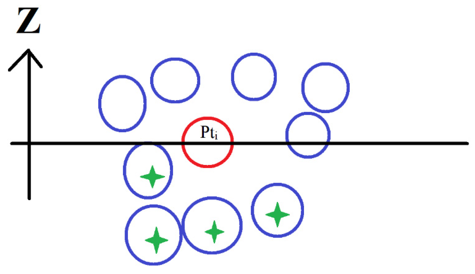
At this point, the number of selected neighboring points n may be related to the point density. However, the algorithm is not sensitive to the variation in the n value. In the tested tree clouds in this paper, the n value is considered to be equal to nine (9). Thereafter, for each detected point
Pti, the n neighboring points are chosen. Only the points having a
Z coordinate value smaller than
ZPti are considered (
Figure 9). This choice has been adopted to avoid detecting multiple stems of the forked trunk.
This algorithm will stop when no additional points can be found. The output will be two point clouds. The first one is the detected stem point cloud and the second is the remaining points. To detect the other stems of the same tree, the remaining point cloud is considered the input point cloud to the same algorithm described above. When the number of remaining points is negligible (less than a given threshold, e.g., 5 points), the stem detection loop stops. Moreover, if the number of points of a detected stem is negligible, the detected stem may represent noisy points and then can be ignored.
Figure 10b illustrates the result of the segmentation of the tree trunk into three single stems. Each stem is independently recognized. At this stage, it is important to note if there are noise points presenting in the trunk point cloud. These points can cause erroneous results for the depicted algorithm, e.g., in
Figure 10c, noise points appear inside the red circle. To eliminate these kinds of noise points, the detected neighboring points must be checked. If the maximum distance between the neighboring points and the considered point is greater than a given threshold, the considered point should be assigned to the noise class. This threshold represents the maximum expected distance between two neighboring points belonging to the same tree trunk, which can be calculated as a function of the point density [
74] and added to a chosen tolerance value. For example, when the point density equals 100 point/m
2, the mean expected distance between two neighboring points is
, and tolerance value is considered equal to 0.1 m; then, the maximum expected distance between two neighboring points equals 0.1 + 0.1 = 0.2 m.
Figure 11 shows the results of the segmentation of different tree trunk point clouds. In this figure, each tree trunk is shown two times. In the first one, the colors are calculated as a function of
Z coordinate values, whereas in the second one, the colors are calculated as a function of the segmentation results of the trunk into individual stems. It is noticed in
Figure 11 that the tested trunks have different levels of complexity, demonstrating the efficiency and flexibility of the suggested algorithm.
4.3. Modeling of Single Stems
Once the tree trunk point cloud is segmented into single stems, the individual stem modeling stage is carried out. In
Section 3.2, it was mentioned that the stem cross-section has variant shapes, and its geometric shape may vary along the same stem. Furthermore, the stem geometric shape is irregular, which is why the suggested approach in this paper divides the tree’s single stem using horizontal planes into small slices and then models each slice independently. Each slice can be represented by a cylinder. The division step should consider the point density where one slice must contain at least the minimal number of points sufficient to model a cylinder. In this paper, the slice height is considered equal to 15 cm where the number of points is between 20 and 40 points per slice. To realize the stem division, it is carried out from the bottom to the top. After extracting each slice of 15 cm height, the number of points on this slice is checked. If it is smaller than the minimum accepted value, which is in this case equal to 10 point/slice, the height of slice is increased to obtain the requested number of points per slice. Mathematically, considering the slice height equals the cylinder height, three points distributed on the cylinder surface are sufficient to fit the cylinder equation. Of course, supplementary measurements may improve fitting results especially when the stem slice does not represent a perfect cylinder. That is why the minimum accepted number of points per slice is taken as equal to 10. Moreover, the value of this threshold can be reduced when the point density value is low. To model one slice, all slice points are projected on a horizontal plane, and then the least squares theory is applied to fit the best circle. This operation allows calculating the cylinder base center as well as the cylinder radius. The cylinder height is equal to the slice height.
At this stage, it is unavoidable to mention that the fitting operation does not always succeed in finding the correct circle parameters that describe the stem geometrical form. Indeed, the cross-section may not be complete because the cloud points do not completely cover the trunk surfaces, and the cross-section is not a perfect circle either. Also, it is supposed that the slice represents a cylinder having a vertical axis, whereas this hypothesis does not always faithfully reflect the reality. Nevertheless, this hypothesis is adopted to realize the best simulation of the trunk’s complicated geometrical shape. To solve the problem of gap-fitting of the slice cylinder, three solutions are suggested. The first one is applying the improved RANdom SAmple Consensuses (RANSAC) paradigm [
75,
76] using clauses that help to detect the best cylinder. These clauses consider the minimum and maximum expected radius regarding the last detected cylinders. The other solution is to check the list of fitted cylinders by comparing each one to its neighboring ones. This operation allows adjusting the cylinder radius values to harmonize with the trunk geometric shape. The last choice is applying the last two methods together, which is adopted in this paper.
5. Results and Discussion
The computer used in this study is Intel® Core™ i7-10610U CPU @ 1.80GHz, 2.30 GHz, RAM 32.0 GB (31.6 GB usable). Moreover, the code is developed and tested under MATLAB 2021b.
As mentioned in
Section 4, after segmenting the tree trunk into single stems, the suggested modeling approach assumes that a tree stem consists of a series of small cylinders. This hypothesis enables us to handle the stem geometrical irregularity. To test the suggested approach, a sample tree point cloud is selected where their trunks are distinguishable and have a complex geometrical shape. Moreover, the selected sample covers all complicated kinds of trunks described in
Section 3.2. At this stage, it is important to note that the developed modeling approach is tested on 38 tree point clouds. The results presented in
Figure 11 and
Figure 12 show the efficiency of the suggested approach as well as its weak points.
From
Figure 12, it can be noted that the tree trunk model consists of a series of connected cylinders of different radius that can construct a 3D shape that describes the trunk geometry. Furthermore, the models illustrated in
Figure 12 belong to different trunk classes such as multiple trunks, forked trunks, oblique trunk, and twisted trunk (see
Section 3.2). Hence, the hypothesis that trunk geometry can be simulated by a group of connected cylinders of different radius confirmed.
Concerning the accuracy estimation, Ostrowski et al. [
77], Cheng et al. [
78], and Tarsha Kurdi and Awrangjeb [
27] recap the accuracy estimation methods of the literature into two families. First, feature-based approaches use a reference model to compare the calculated model. Second, LiDAR-based methods consider the LiDAR point cloud as the reference data. Considering the difficulty of constructing a reference model for the trees, this paper employed the LiDAR-based approach for accuracy estimation. Under this context, the trunk point cloud is superimposed on the constructed trunk model, and then the distances between the LiDAR points and the trunk model are calculated (Equation (4)). These distances represent deviations of LiDAR points from the trunk model. Finally, the standard deviation for each model is calculated (Equation (5) and
Figure 13).
where
are the LiDAR point coordinates,
are the coordinates of the cylinder base circle center,
is the cylinder radius,
n is the number of points of trunk point cloud, and
vi is the point deviations.
Figure 13 exhibits the standard deviations of six 3D tree trunk models presented in
Figure 12 (their numbers in
Figure 13 are from 1 to 6) in addition to another 32 tree point clouds (with a total of 38 tree point clouds). The fact that the number of tested tree point clouds in this paper is small can be explained by the presence of a large number of indistinguishable trunk cases in the available point clouds. Indeed,
Section 3.1 carefully analyzed this issue and cited the main reasons for the indistinguishability of trunk point clouds. In future work, the suggested algorithm in this paper be merged with the crown modeling algorithm suggested by Tarsha Kurdi et al. [
66], and then it will be tested on a vast vegetation dataset.
Sorting the trees by their ID number on the X-axis and using the vertical axis to present the standard deviation values allows for monitoring the fluctuation in the trunk model accuracy from one tree to another and drawing a global impression about the modeling algorithm accuracy. At this point, it shows that the reason for this slight accuracy difference comes from the complexity level of the tree trunk, e.g., when the trunk is twisted or forked, the accuracy drops down by a small amount. However, the modeling accuracy of the selected trees is better than 4 cm, 63% of the mean distance between two neighboring LiDAR points, and thus the model can be considered to produce high-quality results in reference to the employed source data.
The trunk models shown in
Figure 12 represent promising results for high complexity and variation in trunk geometric shapes, which confirms the efficacity of the suggested approach. However, there are limitations for the constructed models. First, the slice cylinders may not be always vertical (see the red arrow in
Figure 12f). Indeed, the slice cylinder axis must be parallel to the stem slop. Second, the cylinder radius may not be always fitted accurately (see
Section 4.3 and the red arrow in
Figure 12e), where the harmonization level between the neighboring cylinder radius must be improved. Finally, gaps between neighboring cylinders must be analyzed and filled (see the red arrow in
Figure 12d). All these can be part of future efforts to improve the proposed modeling algorithm.
At this stage, it is beneficial to compare one tree trunk model with the real image of the tree. For this purpose, the tree illustrated in
Figure 5f is considered. From
Figure 14, it can be noted that the suggested algorithm succeeds in generating the tree trunk model by conserving its geometrical shape, where the tree trunk consists of three stems, two of which form a forked branch and the third represents a sloped branch. Moreover, the trunk diameter, especially at the connection of two stems, is not accurate enough, and it looks slightly greater than the reality. Indeed, the LiDAR points partially cover the tree trunk, and then fitting the best cylinder at the stem junction may cause a considerable error (see red arrow in
Figure 14d). Also, the presence of some leaves connected to the trunk could be considered as part of the trunk and consequently generate an error in the trunk diameter (see the blue arrow in
Figure 14d). Finally, at the bottom of the trunk, where it connects to the soil, it may have a small deformation (see the green arrow in
Figure 14d). Indeed, the lower part of the trunk does not fit the used hypothesis that the trunk has approximately a cylindrical geometric shape. However, the division of the trunk point cloud into small cylinders and modeling them separately helps to reduce the modeling errors and make them appear only locally.
As the proposed algorithm is developed to complete the tree crown modeling algorithm suggested by Tarsha Kurdi et al. [
66], it is unavoidable to illustrate the result of tree modeling using the updated tree modeling algorithm (
Figure 14e).
Figure 14e confirms the success of the trunk modeling approach because the trunk modeling errors are negligible regarding the great volume of the tree compared to the trunk volume.


