Inversion Study of Nitrogen Content of Hyperspectral Apple Canopy Leaves Using Optimized Least Squares Support Vector Machine Approach

Abstract

The rapid and accurate estimation of the nitrogen content of fruit trees helps to achieve a precise management of orchards. Hyperspectral data were collected from leaves of apple tree canopies at different fertility stages through field experiments to investigate the relationship between the nitrogen content and spectral reflectance of apple canopy leaves. Two different preprocessing methods, Savitzky–Golay (SG) smoothing and multiple scattering correction (MSC), were used to extract the feature bands by combining the successive projection method (SPA) and the competitive adaptive weighting algorithm–partial least squares (CARS-PLS). The reflectance values of the feature bands screened via these two methods were used as inputs to construct the multi-factor inversion models of apple canopy leaf nitrogen content based on the long- and short-term memory (LSTM) network, the support vector regression (SVR) and the Least Squares Support Vector Machine Regression (RIME-LSSVM). The study compared the ability of three algorithmic models to estimate leaf nitrogen content, and the results showed that the model constructed with the reflectance values of the characteristic bands screened by the CARS-PLS algorithm as inputs was more effective in predicting the nitrogen content of leaves. Furthermore, the accuracy of the model constructed using RIME-LSSVM was significantly higher than that of the model constructed using the long- and short-term memory network and support vector regression, in which the coefficient of determination of the test set (R-squared) is 0.964 and the root-mean-squared error (RMSE) is 0.052. Finally, the CARS-PLS algorithm combined with the RIME-LSSVM model has a higher prediction accuracy. The study demonstrated the feasibility and reliability of hyperspectral techniques for the estimation of nitrogen content of apple leaves in the Aksu region.

1. Introduction

The fruits of Rosaceae apple plants are rich in vitamins and minerals. China is the world’s largest producer of apples, with production reaching 48 million tons in 2022. Xinjiang is one of China’s most important apple production areas, with a long cultivation history [1]. The total area under cultivation has reached 390,000 mu, making apples an important cash crop in the Ring Tarim Basin that play a positive role in helping farmers to increase their income [2].

Nitrogen is one of the most important elements affecting the growth and development of apples. A lack of nitrogen causes the yellowing and curling of leaves, which has an impact on the quality of the fruits and can even result in the phenomenon of early fruit drop [3]. Meanwhile, excessive use of nitrogen fertilizers reduces the sugar content of the fruits and exacerbates the problem of soil acidification, which affects sustainable development [4]. Therefore, timely and accurate access to the nitrogen content of the leaves at the apple crown can facilitate the real-time management of orchards by providing information on growth and allowing for continued monitoring [5].

Traditional methods of plant nitrogen determination require that plant samples collected in orchards are brought back to the laboratory, ground, and treated with chemical reagents to determine their nitrogen content using formaldehyde [6] and distillation [7] methods. The formaldehyde method is an indirect titration of the acid–base titration method, where formaldehyde interacts with an ammonium salt and undergoes a formaldehyde–ammonia reaction, and the resulting compound is measured via colorimetry to determine the color of the solution. The amount of nitrogen in the sample can be indirectly determined; however, operating conditions must be strictly controlled, otherwise it is easy to produce large errors [6]. The distillation method obtains the nitrogen concentration by distilling out the nitrogen in the water sample and neutralizing and titrating it with a standard hydrochloric acid solution, which gives accurate and reliable results; however, the operation is cumbersome and time-consuming, and if the purity of the sample is poor, the analytical results are often low [7]. Hyperspectral remote sensing has the advantage of rapidly and non-destructively acquiring the canopy spectral information of crops, as compared to traditional determination methods [8,9]. Spectral analysis and nutritional diagnosis are carried out by utilizing the different degrees of light absorption and reflection by crop leaf cells, pigments, and water content [9]. Since nitrogen content and chlorophyll are closely related, a nitrogen content that is too low will lead to slowing down the rate of chlorophyll synthesis in crop leaves. Chlorophyll has a strong absorption rate in the red and blue light bands, and at the same time, the shape and position of the red edge band will be changed with the lack of nitrogen, so that a spectral nutrient diagnosis of the nitrogen content of the crop can be carried out accordingly [9]. Hyperspectral technology has been widely used for nutrient estimation in crop leaves, which is currently a focus of precision agriculture research [8,9].

Hyperspectral data in the acquisition process usually bear certain issues such as a large volume, redundancy, duplication, noise, as well as other problems. Therefore, in order to solve these problems so as to improve data quality, the data used in the prediction accuracy of the model to produce certain constraints should be preprocessed. Previous studies have shown that the preprocessing of spectral data can effectively reduce noise decomposition; therefore, extracting the sensitive bands of nitrogen spectra and constructing the model can improve the model accuracy. Ma et al. [10] explored the possibility of using hyperspectral techniques for the detection of total soil nitrogen, SG smoothing, and MSC spectral data preprocessing, combined with five modeling methods—partial least squares (PLS), back propagation (BP) neural network, radial basis function (RBF) neural network, extreme learning machine (ELM), and SVR—to compare the errors of spectral analysis using chemical analysis results as a control. The results showed that all five models could be used for the detection of soil total nitrogen content, and the SG smoothing preprocessing model had a better detection ability compared with MSC, with an R-squared of 0.8767, and an RMSE of 1.302, among which the SVR model had the best accuracy, with an R-squared of 0.9121 and an RMSE of 0.7581.

Since hyperspectral data have high-dimensional characteristics, and a lot of wavelength information in the visible and near-infrared spectra may be irrelevant to the target, the extraction of feature bands can reduce the bias caused by irrelevant wavelength information and improve the model prediction accuracy [11]. For example, the SPA algorithm can effectively extract feature bands from severely overlapping spectra, thus minimizing the effect of reducing covariance between spectral variables [12]. The CARS-PLS algorithm rejects redundant information by filtering feature selection [13]. Previous studies have shown that nonlinear models have more obvious advantages than linear models in quantitative prediction [14,15]. Common nonlinear models include SVR, LSTM, and RIME-LSSVM [16,17,18]. Therefore, this study further explores nonlinear modeling methods applicable to the prediction of leaf nitrogen content in apple trees.

To date, hyperspectral-based nitrogen inversion studies have mostly focused on wheat, rice, soybean, corn, and other grain crops. For example, Bruning et al. [19] have conducted nitrogen content inversion studies on hyperspectral data for four different genotypes of wheat through multiple regression methods combined with 10 spectral preprocessing techniques, and the results showed that the nitrogen content in the visible and near-infrared bands of 400–1000 nm was predicted with a 0.59 accuracy of R-squared. The prediction model accuracy was improved by adding the shortwave infrared band of 1000–2500 nm, providing an R-squared of 0.66, indicating that the red-edge band has a better effect for nitrogen content prediction. Guo et al. [20] took different varieties of winter wheat as the research object, used the continuous wave removal method to expand the characteristic band of nitrogen uptake, analyzed the correlation with leaf nitrogen accumulation (LNA), and compared the prediction accuracy of three nonlinear modeling methods for LNA. Their results showed that the continuous wave removal method improved the correlation with the LNA, and the Support Vector Machine (SVM) regression model had a higher accuracy with an R-squared of 0.8950. Yu et al. [21] investigated the relationship between nitrogen (N) content and spectral reflectance difference of rice in cold land, established a hyperspectral reflectance difference model for the difference in N content of rice, and modeled the spectral data by combining the PLS, the ELM, and the genetic algorithm-extreme learning machine (GA-ELM) algorithms after processing the spectral data using the discrete wavelet multi-scale decomposition, the continuum projection algorithm, and the principal component analysis. The results show that the GA-ELM model established via discrete wavelet multiscale decomposition obtains optimal results in both dataset modeling and training, and the R-squared of both training and validation datasets are above 0.68.

Hyperspectral techniques for nutrient element monitoring in fruit trees have also been studied by previous researchers, such as Azadnia et al. [22], who combined visible/near-infrared spectroscopy with four different machine learning algorithms, namely SVM, artificial neural networks (ANNs), Random Forest (RF), and PLS, to predict N, phosphorus (P), and potassium (K) contents in apple leaves. The results showed that the nonlinear modeling approach outperforms the linear one in all models. Gómez-Casero et al. [23] combined hyperspectral reflectance curves of olive trees under different nitrogen and potassium treatments, as well as the optimal wavelengths for distinguishing between different nitrogen and potassium treatments to explore the changes in the nutrient content of olive tree leaves in vegetation indices, with an accuracy of up to 94.4%, and the results showed that nitrogen or potassium nutritional deficiencies in olive tree leaves are mainly concentrated in the near-infrared region of hyperspectral reflectance. Somers et al. [24] collected spectral data on fruit tree leaves, fruits, and canopies in citrus orchards and cross-referenced them with biophysical and biochemical characteristics of the trees to explore the effect of citrus fruits on the spectral reflectance of canopies. The results showed that the presence of fruit resulted in a significant decrease in reflectance in the infrared region (700 to 2500 nm) of the electromagnetic spectrum. In the visible (VIS: 350 to 700 nm) region, the fruit had less effect, mainly due to leaf chlorosis resulting from nitrogen competition between canopy elements. Einzmann et al. [25] conducted two years of field monitoring of Norway spruce forests to explore the effects of artificial stress (bark stripping) on tree vigor in conjunction with hyperspectral data, transforming needle and canopy spectra with spectral derivatives, vegetation indices, and angular indices, and checking the separability of all features (ring-barked trees vs. control trees) using an RF classification algorithm. The results showed that younger, well-maintained stands showed less change over the 2-year period, while the changes in older stands were observed in both coniferous and hyperspectral canopy spectra, suggesting the great potential of hyperspectral remote sensing in detecting early vigor changes in stressed trees. In contrast, there have been fewer studies on the use of hyperspectral technology for the determination of apple physiological and biochemical indices; therefore, the use of hyperspectral technology for monitoring apple growth information in the Tarim Basin of the Southern Xinjiang Ring still needs to be further discussed.

In this study, the spectral raw data were preprocessed via SG smoothing and MSC, and the feature variables of the bands were extracted using CARS-PLS and SPA algorithms. Based on the feature variables extracted with the above two methods, the prediction accuracies of the three models (SVR, LSTM, and RIME-LSSVM) were established and compared, and the optimal model for estimating the nitrogen content of the canopy leaves of apple trees was determined.

2. Materials and Methods

2.1. Overview of the Study Area

Shahe Town, Aksu Region, Xinjiang Province, is located in the northern edge of the Tarim Basin; geographic coordinates are 41°12′30″–41°24′30″ north latitude, and 80°47′15″–80°57′ east longitude. The irrigation area has a typical continental climate, with large temperature differences between day and night. The average annual sunshine is 2621 h, the average annual precipitation is 79.3 mm, and the average annual frost-free period is 202 days. The climate is mild, rich in heat, and abundant in light. The soil type was sandy, in which the soil organic matter content was 11.05 g/kg; effective phosphorus content was 3.2 mg/kg; quick-acting potassium content was 33 mg/kg; alkaline-dissolved nitrogen (ADN) and total nitrogen (TN) content were 10 mg/kg and 176 mg/kg, respectively. pH value was 8.71, making it more suitable for growing apples.

2.2. Data Acquisition

2.2.1. Apple Canopy Leaf Hyperspectral Data Acquisition

Hyperspectral data of apple tree canopy leaves were collected using an ASD FieldSpec HandHeld2 portable spectroradiometer (Analytical Spectral Devices, Boulder, CO, USA). Spectral data were collected from May to September 2023 during the full apple growing season. Spectral data from all canopy leaves were collected under clear, windless, cloudless, and stable light conditions, with a solar altitude angle greater than 45°, and from 10:00 to 14:00 on the same day to ensure the accuracy of the spectral data. The spectrometer needed to be calibrated with a whiteboard before data collection and every 15 min, and the results of the calibration required that the spectral reflectance in the range of bands were all 1. During the acquisition process, the sample leaves were placed against a black background, the instrument probe was vertically downward and always kept 15–20 cm away from the sample, and the spectrometer field of view was 25°. When measuring the spectra, the experimenter had to wear dark-colored clothes facing the direction of sunlight to avoid shadows or light-colored reflections affecting the spectral characteristics of the leaves, and at the same time, they had be careful to avoid the measurement of leaf veins. Twenty spectral curves were collected for each sample leaf, and the average value was taken as the final reflectance information of the sample. The spectral reflectance data were collected using ViewSpecPro 6.2.0 (ASD Inc., Boulder, CO, USA) software.

2.2.2. Determination of Nitrogen Concentration in Apple Canopy Leaves

Leaves from which spectral data had been collected were placed in self-sealing bags to await determination of the nitrogen content of the leaves. The leaves were placed in an oven at 105 °C for 30 min for de-enzymatic treatment; then, the oven temperature was adjusted to 80 °C and the leaves were baked until they were of constant weight. The dried samples were ground into powder, weighed 0.2 g, digested and treated with H2SO4, and then the total nitrogen content of the samples was determined using a KjeltecTM 8400 Kjeldahl Nitrogen Analyzer (FOSS, Inc., Hilleroed, Zealand, Denmark) [26].

2.2.3. Spectral Data Preprocessing

During the acquisition of hyperspectral data, due to the effects of baseline drift, sample inhomogeneity, scattering, and human manipulation, the spectral curve of the signal contained a small amount of noise [27]. SG smoothing does not change the shape or width of the signal when filtering noise [28], while multiplicative scatter correction (MSC) can effectively eliminate the spectral differences due to different scattering levels, thus enhancing the correlation between the spectral reflectance and nitrogen content [29]. In view of this, the two methods were combined to perform noise reduction on the spectral data. The SG-smoothed image had the same shape as the original image, while MSC removed the spectral differences by correcting the baseline translation and offset phenomena of the SG-smoothed spectral data with the ideal spectrum (Figure 1).

After removing the error samples, 165 sets of valid data were finally retained. These 165 sets of data were divided into a training set (containing 120 groups) and a test set (containing 45 groups) using the SPXY algorithm [30]. The maximum value of the total sample was 2.851 mg/g, the minimum value was 1.136 mg/g, the mean value was 2.165 mg/g, the standard deviation was 0.578, and the coefficient of variation was 26.7%. The maximum value of the training set samples was 2.851 mg/g, the minimum value was 1.136 mg/g, the mean value was 2.085 mg/g, the standard deviation was 0.523, and the coefficient of variation was 25.1%. The maximum value of the test set was 2.734 mg/g, the minimum value was 1.412 mg/g, the mean value was 2.073 mg/g, the standard deviation was 0.636, and the coefficient of variation was 30.7%. It can be seen that the coefficients of variation are all less than 35%, basically conforming to normal distribution.

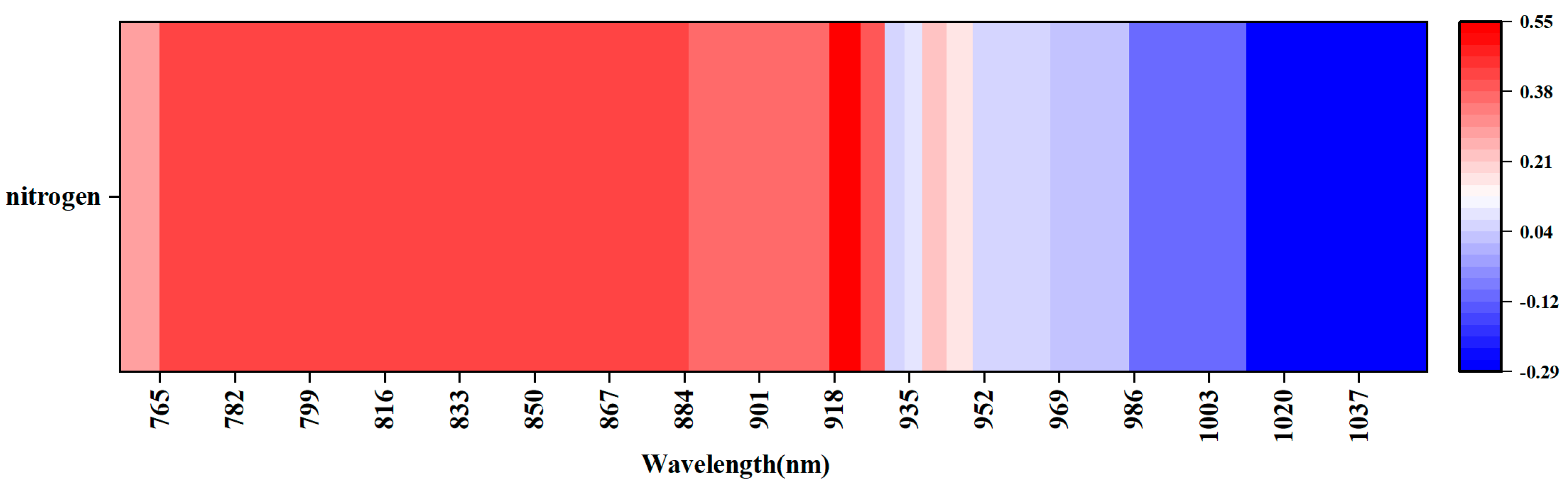
2.3. Selection of Spectral Characteristics of Apple Leaves

The dataset after spectral preprocessing was still a high-dimensional dataset, for which subsequent processing is difficult due to the high redundancy of information and high correlation between different spectral bands. Thus, selecting appropriate features from the spectral data is the key to improving the accuracy of the resulting model.

We used two methods for feature selection: The SPA method and the CARS-PLS method. The SPA method is a forward iterative selection method that utilizes projection analysis of vectors to select the effective wavelength with the least amount of redundancy as a means to solve the covariance problem, thus reducing the number of model inputs and achieving a reduction in the training time of the model [15,31]. The CARS-PLS method is a dimensionality reduction method based on the regression coefficients of the partial least squares model. The wavelength points in the PLS model with large regression coefficients (in terms of absolute value) are selected as a new subset each time, using an adaptive re-weighted sampling technique [32,33]. A PLS model is constructed based on the new subset, and the subset with the lowest root-mean-squared error of model cross-validation (RMSECV) is screened out as the characteristic wavelength through multiple calculations. The inversion model is then constructed by taking the spectral matrix of the sample data and the spectral matrix of the random noise matrix mixing as the input. In this study, the CARS-PLS algorithm was set to run 100 times with 20 sets of interactive validation.

2.4. Algorithm Fundamentals

2.4.1. Long- and Short-Term Memory Networks

Long short-term memory (LSTM) is a type of recurrent neural network (RNN); however, compared with RNNs, it includes more gating units (including forget gates, input gates, and output gates). These can selectively memorize historical data and improve the long-term memory ability of the neural network, effectively overcoming the problems of gradient vanishing and gradient explosion that occur in RNNs during training [34]. LSTM neural networks usually use sigmoid and tanh as the activation functions, and the LSTM memory cell calculation formula can be expressed using the following equations [35]:

$$f_t=\sigma \left({\omega }_{ix}{x}_t+{\omega }_{fh}{h}_{t-1}+{\omega }_{fc}{c}_{t-1}+b_f\right)$$

(1)

$$i_t=\sigma \left({\omega }_{ix}{x}_t+{\omega }_{ih}{h}_{t-1}+{\omega }_{ic}{c}_{t-1}+b_i\right)$$

(2)

$$o_t=\sigma \left({\omega }_{ox}{x}_t+{\omega }_{oh}{h}_{t-1}+{\omega }_{oc}{c}_{t-1}+b_o\right)$$

(3)

$$c_t=f_t{c}_{t-1}+i_t\mathit{tanh}\left({\omega }_{cx}{x}_t+{\omega }_{ch}{h}_{t-1}+b_o\right)$$

(4)

$$h_t=o_t\mathit{tanh}\left(c_t\right)$$

(5)

In Equations (1)–(5), $f_t$ denotes a forget gate, which controls the parts that are forgotten, and $\sigma$ is the sigmoid function [36]:

$$\sigma \left(x\right)=\frac{x}{1+e^{-x}}.$$

(6)

In the sigmoid function, negative infinity is mapped to a value of 0, which means that the data are not activated, and positive infinity is mapped to a value of 1, which means that the data are fully activated.

Furthermore, $h_{t-1}$ is the hidden-layer state at moment $t-1$; $x_t$ is the input feature vector at moment $t$; ${\omega }_{ix}{{\omega }_{fh}\omega }_{fc}{\omega }_{ih}{\omega }_{ic}{\omega }_{ox}{\omega }_{oh}{\omega }_{oc}{\omega }_{cx}{\omega }_{ch}$ are weight matrices; $b_f{b}_i{b}_o$ are error vectors, which are mainly used to establish the connections between the input layer, the output layer, and the storage; $i_t$ denotes an input gate, which controls which parts are used as input and determines whether or not the input data are ignored; $o_t$ denotes an output gate, which controls the output of the message and determines whether the hidden state is used; and $c_t$ is the neuron state. The hidden-layer state variable at moment t can be calculated using Equation (5), and $tanh$ denotes the hyperbolic tangent activation function [36], given by:

$$\mathit{tanh}x=\frac{\mathit{sinh}x}{\mathit{cosh}x}=\frac{e^x-e^{-x}}{e^x+e^{-x}}$$

(7)

In this study, the model was set to have an initial learning rate of 1 × 10⁻² and a learning rate of 0.01 × 0.5 after 800 training sessions.

2.4.2. Support Vector Regression

Support Vector Machine (SVM) is a machine learning algorithm based on supervised learning that has been widely used for the classification and regression of hyperspectral data. SVM uses a kernel function to map the original data from the original space to a new feature space, where a linear method is utilized to learn from the training data to solve a nonlinear problem [37]. The sigmoid kernel function, polynomial kernel function, linear kernel function, and radial basis function (RBF) are the four main kernel functions used in SVM models. In this study, based on a priori knowledge, the RBF kernel function was chosen. The formula of the SVM model is as follows:

$$f\left(x\right)=sgn\left({\sum }_{i=1}^M{y}_i{a}_{i}k\left(x_i,x\right)+\delta \right)$$

(8)

where $y_i$ denotes the classification label, $a_i$ is the Lagrange coefficient, M denotes the sequence of data vectors, $\delta$ is the threshold, and $k\left(x_i,x\right)$ represents the kernel function of the SVM model.

Support vector regression (SVR) is a model for the application of SVM to regression problems. The core idea is to find a hyperplane such that the total deviation of all sample points from that hyperplane is minimized [38]. The SVR model is formulated as follows:

$$f\left(x\right)=\left({\sum }_{i=1}^M\left(\widehat{a_i}-a_i\right)k\left(i_T^x,x\right)+b\right)$$

(9)

In this study, the penalty factor of the SVR model was set to 4.0 and the radial basis function parameter was set to 0.8.

2.4.3. Least Squares Support Vector Machine Algorithm

SVM is not prone to overfitting when dealing with small training sets, and its performance is superior to that of many artificial neural networks in this case. However, when faced with larger datasets, SVMs take longer to train. Therefore, in order to improve the training efficiency of SVM, Suykens et al. [39] have proposed the Least Squares Support Vector Machine (LSSVM). LSSVM inherits many of the advantages of SVM while outperforming the original SVM in terms of computational efficiency.

Given a training set ${i=1}_N^{\left\{\left(x_i,t_i\right)\right\}}$, where $x_i\in R^m$ denotes m-dimensional factors affecting slope displacement and $t_i\in R$ denotes an actual measured value of slope displacement, the LSSVM for regression analysis can be expressed as a constrained optimization problem using the following equation:

$${min}_{\omega ,b,\epsilon }J\left(\omega ,\epsilon \right)=\frac{1}{2}{\omega }^T\omega +\frac{1}{2}\gamma {\sum }_{i=1}^N{\epsilon }_i$$

(10)

$$\mathrm{such} \mathrm{that} t_i={\omega }^T\mathrm{\varnothing }\left(x_i\right)+b+{\epsilon }_i,i=\mathrm{1,2}\dots ,N,$$

(11)

where $\gamma$ is the regularization parameter, ${\epsilon }_i$ represents the random error, ${\omega }^T$ is the weight vector, and b is the threshold. The solution is shown in Equation (12):

$$t\left(x\right)=sign\left({\sum }_{i=1}^N{a}_{i}K\left(x_i,x_k\right)+b\right)$$

(12)

where $a_i$ is the Lagrange multiplier and $K\left(x_i,x_k\right)$ is the kernel function matrix.

2.4.4. Frost and Ice Optimization Algorithm (RIME)

The RIME algorithm proposes a soft fog search strategy, mainly by simulating the movement of soft fog particles. By simulating the crossover behavior among hard fog agents, a hard fog puncturing mechanism is proposed in the development step of the algorithm. For the five motion characteristics of haze particles, the condensation process of each particle is briefly simulated, and the position of nuclear particles is calculated as detailed in Equation (13). Finally, the selection mechanism of the meta-heuristic algorithm was improved and a positive greedy selection mechanism was proposed to avoid becoming trapped in local optima [40].

$${i,j}_{new}^R=R_{best,j}+r_1·\mathit{cos}\theta ·\beta ·\left(h·\left(u{b}_{ij}-L{b}_{ij}\right)+L{b}_{ij}\right),r_2<E$$

(13)

where ${i,j}_{new}^R$ is the new position of the updated particle, i and j index the haze agents and particles, respectively, and R_best,j is the jth particle of the best haze agent in population R.

$$\theta =\pi ·\frac{t}{10·T}$$

(14)

where $t$ is the current number of iterations and $T$ is the maximum number of iterations of the algorithm.

$$\beta =1-\left[\frac{\omega ·t}{T}\right]/\omega$$

(15)

In Equation (15), the mathematical model of $\beta$ is a step function, and $\left[·\right]$ denotes rounding. The default value of $\omega$ was 5, which was used to control the number of segments of the step function. Returning to Equation (13), $u{b}_{ij}$ and $L{b}_{ij}$ are the upper and lower bounds of the escape space, respectively, which limit the effective region of particle motion; and E is the coefficient of attachment, which affects the coagulation probability of the agent and increases with the number of iterations, as defined in Equation (16):

$$E=\sqrt{\left(t/T\right)}$$

(16)

In this study, the number of populations was set to 30 and the 30 iterations are independently parallelized.

2.5. Evaluation Metrics

In order to fully evaluate the performance of the model, the coefficient of determination (R-squared) and root-mean-squared error (RMSE) are selected to assess the prediction precision and accuracy of the model. In general, a satisfactory model should have a high R-squared and a low RMSE. The closer R-squared is to 1, the better the model’s ability to explain the dependent variable; the smaller the RMSE, the higher the model’s precision and estimation ability. The calculation formulae are as follows:

$$R^2=1-\frac{{\sum }_{i=1}^n{\left(y_i-{\widehat{y}}_i\right)}^2}{{\sum }_{i=1}^n{\left(y_i-{\overline{y}}_i\right)}^2}$$

(17)

$$RMSE=\sqrt{\frac{{\sum }_{i=1}^n{\left(y_i-{\widehat{y}}_i\right)}^2}{n}}$$

(18)

Here, ${\widehat{y}}_i$ is the predicted value, $\overline{y}$ is the mean of the observed values, $y_i$ is the observed value, and $n$ is the number of samples.

3. Results

3.1. Selection of Features

3.1.1. Selection of Features by Continuous Projection Method

The results of screening apple canopy leaf spectral features using the SPA method showed that the cross-validated RMSE gradually decreased with the increase in the number of features, reached a minimum at 47 features (equal to the number of bands), and then showed an upward trend (Figure 2). It can be seen that too few or too many characteristic bands are not favorable for the correct determination of the nitrogen content of apple canopy leaves; thus, the optimal number of spectral bands was determined to be 47. These bands were distributed between 405 and 1050 nm and were 729, 723, 992, 856, 923, 953, 755, 932, 801, 933, 1000, 330, 1022, 967, 849, 944, 877, 1002, 413, 806, 980, 1006, 1011, 1004, 994, 659, 931, 968, 973, 826, 956, 998, 917, 969, 971, 1019, 1007, 1015, 756, 925, 982, 913, 976, 983, 948, 987, and 975 nm. The correlation analysis of the 47 extracted characteristic bands with nitrogen showed that the band with the highest correlation with nitrogen was 330 nm (Figure 3). The reflectance values corresponding to these selected characteristic wavelengths were introduced into the three models as independent variables for multi-factor inversion.

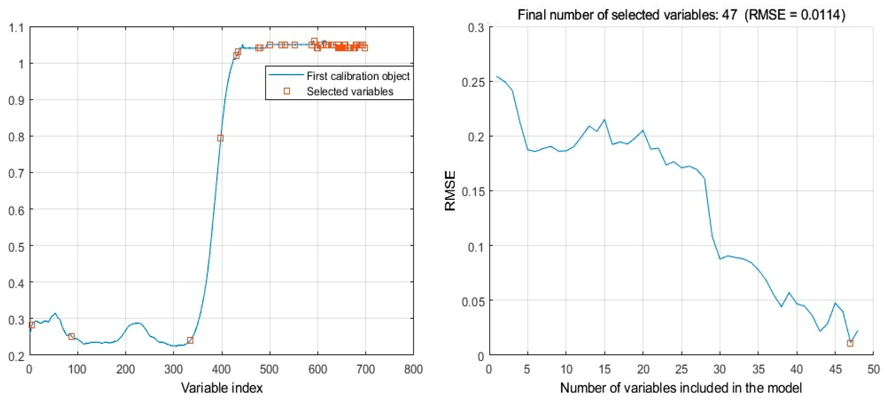
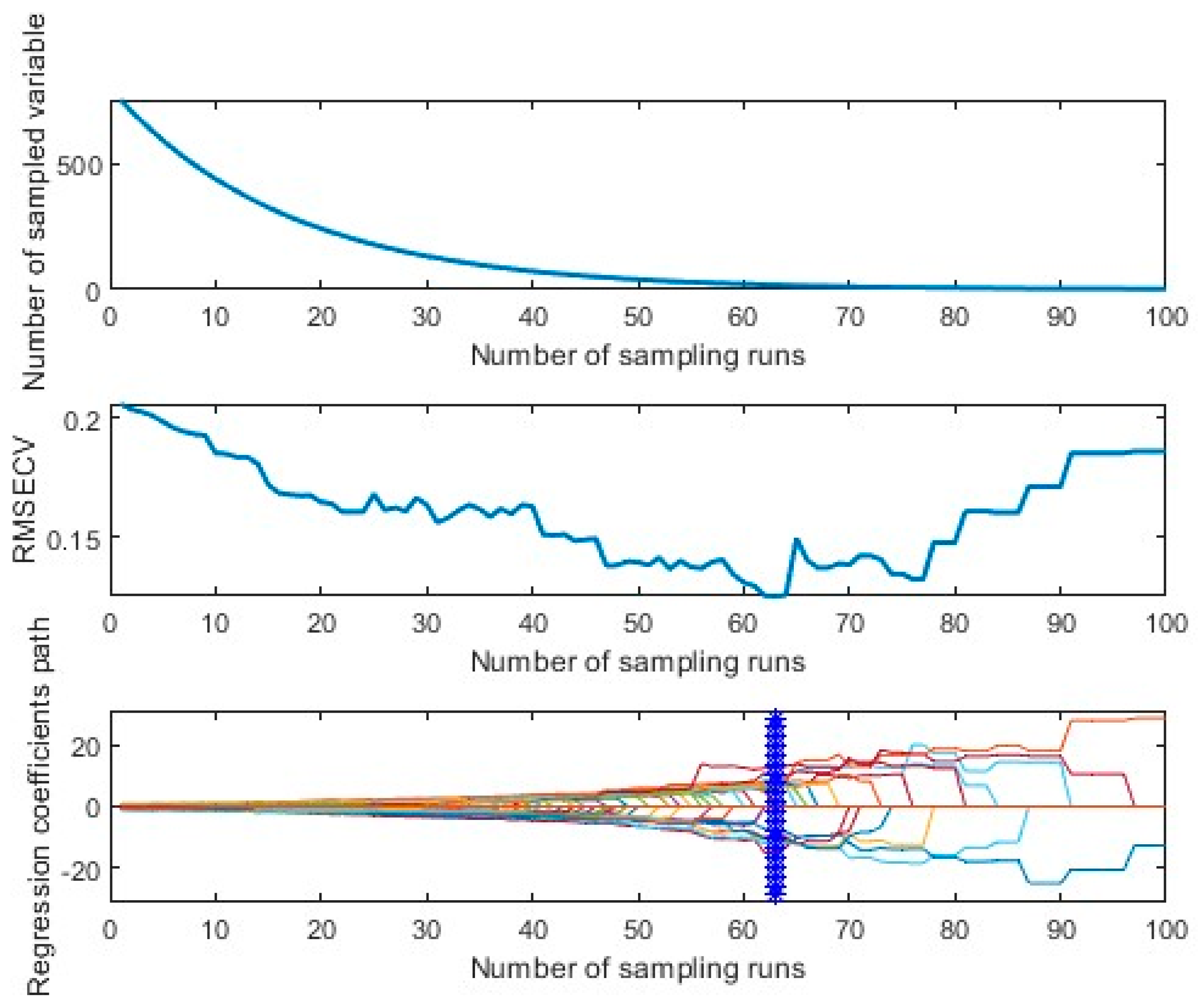
3.1.2. Competitive Adaptive Re-Weighting Method–Partial Least Squares

The variable screening process for CARS-PLS showed a gradual decrease in the number of variables as the number of variable runs increased (Figure 4). As the number of runs increased from 1 to 63, the root-mean-squared error of the cross-validation (RMSECV) decreased gradually. When the number of runs was 63, the minimum RMSECV value was obtained. However, after 63 runs, the RMSECV increased gradually with an increase in the number of runs, which may be due to the fact that, as the number of runs increased, the CARS-PLS algorithm removed the bands that were more or less correlated with leaf nitrogen content (LNC) bands with strong correlation, leading to a decrease in the accuracy of the constructed PLSR model. The paths of the regression coefficients of the spectral variables show that the changes in the regression coefficients leveled off and converged to a stable value when the number of samples was between 1 and 63. With a continued increase in the number of samples, the regression coefficients showed some fluctuations, and the RMSECV reached its minimum when the number of samples was 63, indicating that the CARS-PLS method has good stability and its results are reliable. The number of wavelengths was reduced from 751 to 18 after screening with CARS-PLS variables—about 0.23% of the full band. These bands were distributed between 755 and 1035 nm and were 757, 759, 771, 856, 857, 858, 912, 922, 926, 933, 935, 941, 943, 944, 955, 979, 991, and 1032 nm. The correlation analysis of the 18 characteristic bands extracted with nitrogen showed that the highest correlation band with nitrogen was 922 nm (Figure 5). The reflectance values corresponding to these selected characteristic wavelengths were introduced into the three models as independent variables for multi-factor inversion.

3.2. Inverse Modeling and Analysis of the Apple Leaf Nitrogen Content

3.2.1. Inverse Modeling Based on the Long Short-Term Memory Network, Support Vector Regression, and the RIME Optimization Algorithm Based on Least Squares Support Vector Machine Regression

After the spectral reflectance of the apple canopy leaves was downscaled using two methods—namely the SPA algorithm and CARS-PLS algorithm—the reflectance of the selected features was used as the independent variable of the models, while the nitrogen content of the apple canopy leaves was used as the target variable. Inversion models based on a long short-term memory network, support vector regression, and the RIME optimization algorithm based on Least Squares Support Vector Machine Regression (RIME-LSSVM) were constructed, and the optimal number of iterations was taken according to the different models to obtain the best results for each of the three models (

Table 1. Inversion model evaluation indicators.

Extraction Method Characteristics	Inversion Model	R-Squared		RMSE
		Training Set	Test Set	Training Set	Test Set
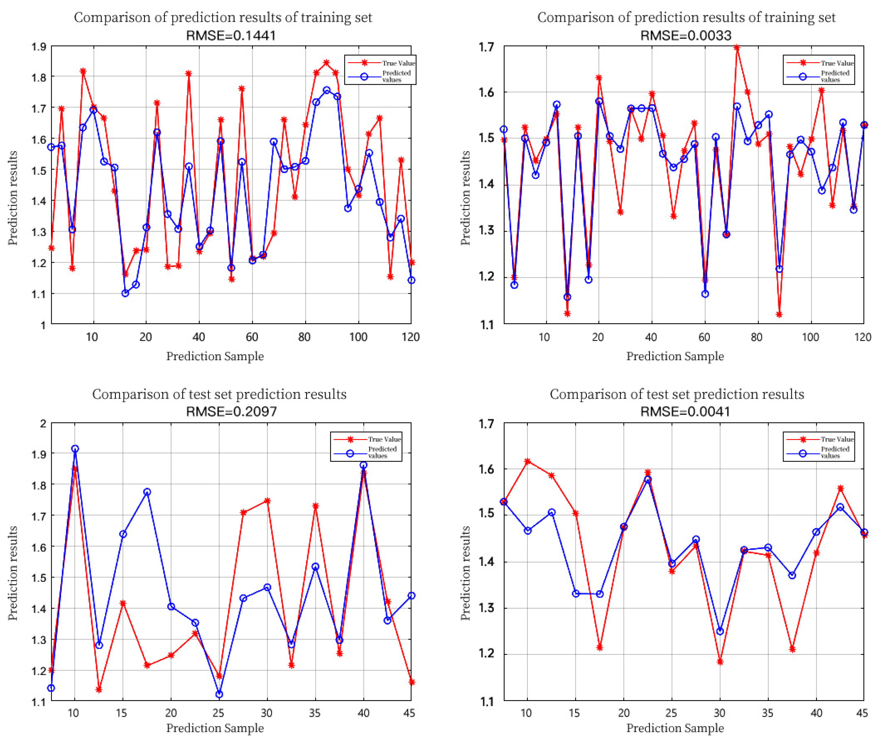
SPA	LSTM	0.6506	0.3307	0.1441	0.2097
CARS-PLS	LSTM	0.7862	0.6155	0.0033	0.0041
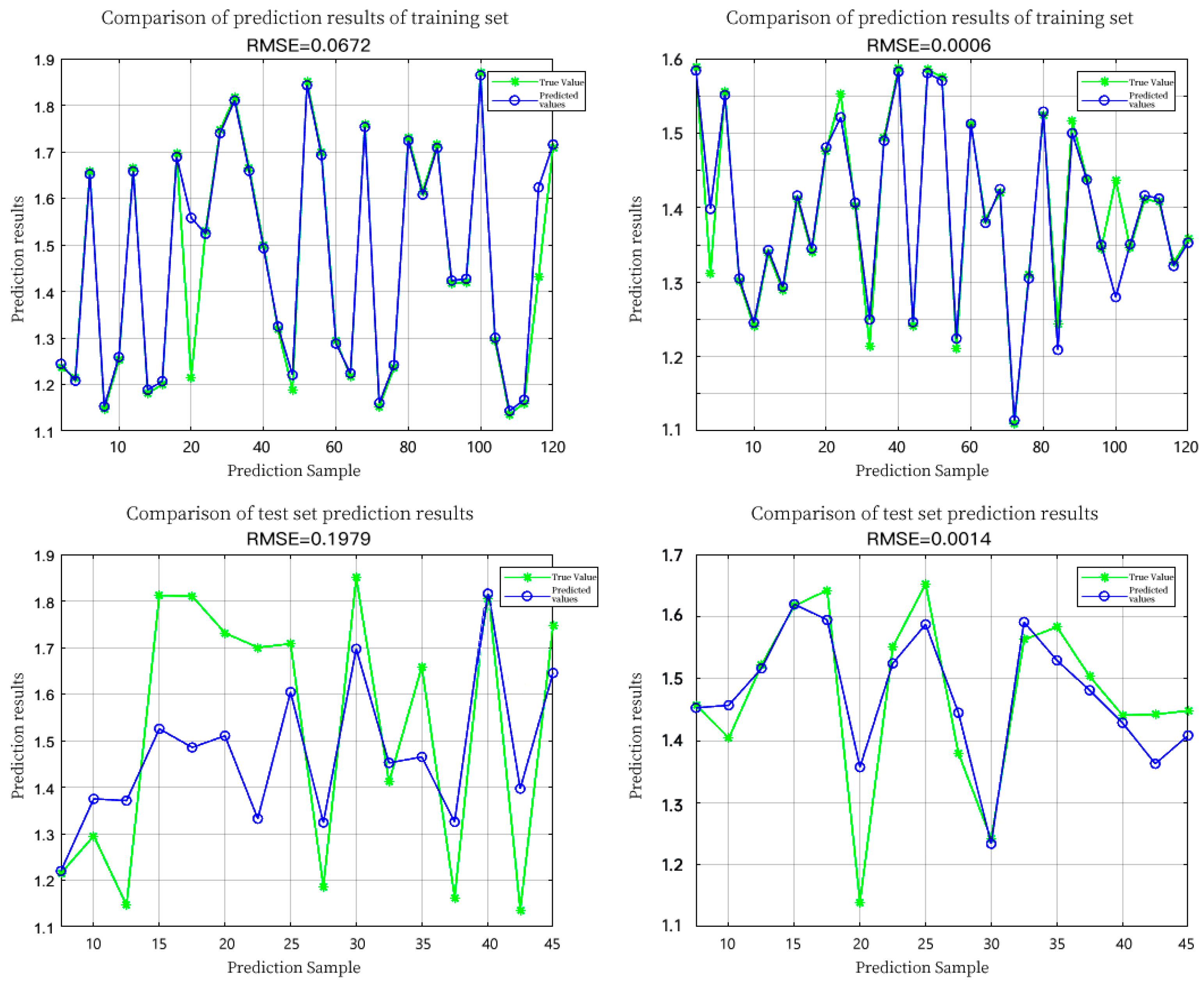
SPA	SVR	0.9238	0.4966	0.0672	0.1979
CARS-PLS	SVR	0.9306	0.7468	0.0006	0.0014
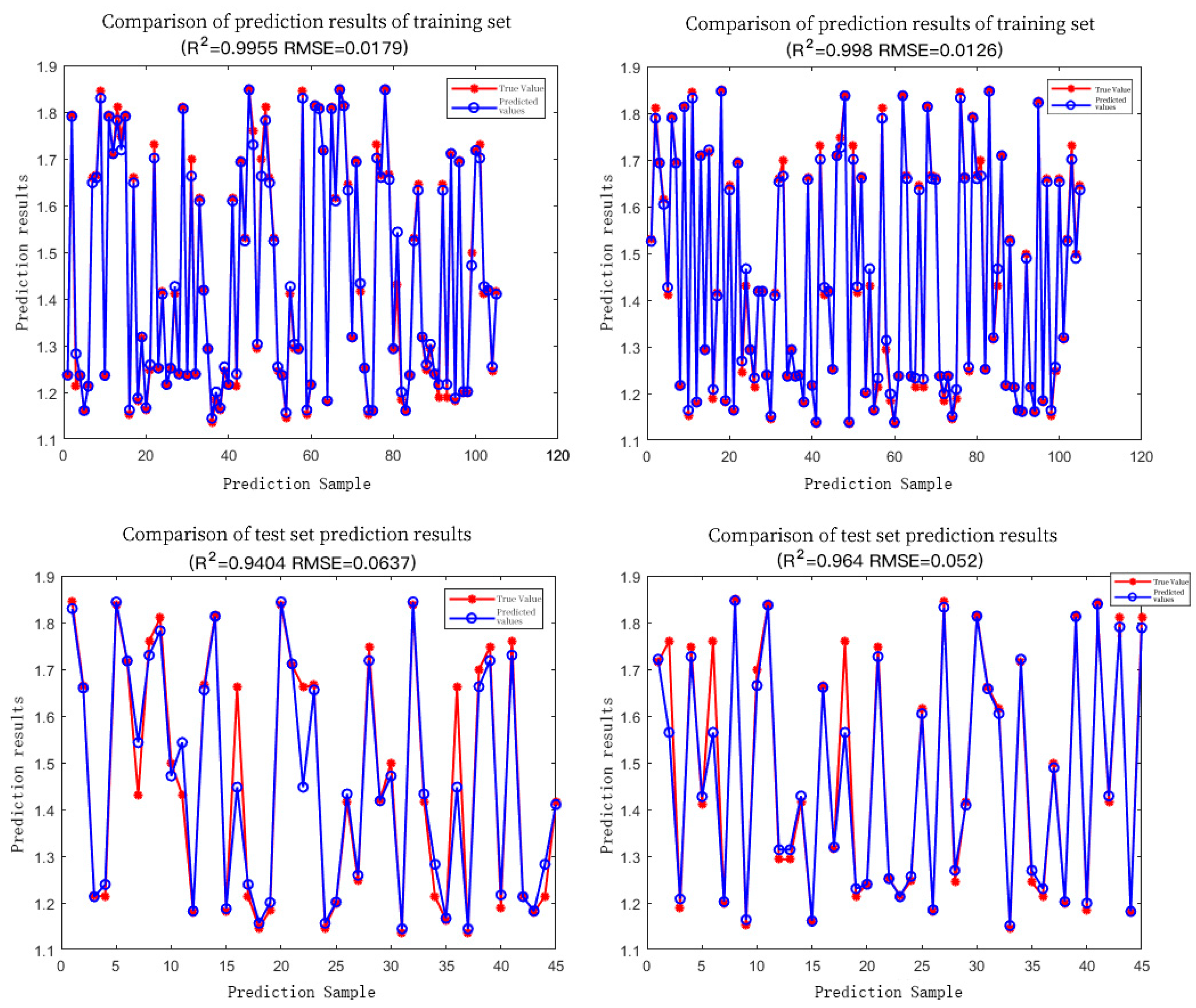
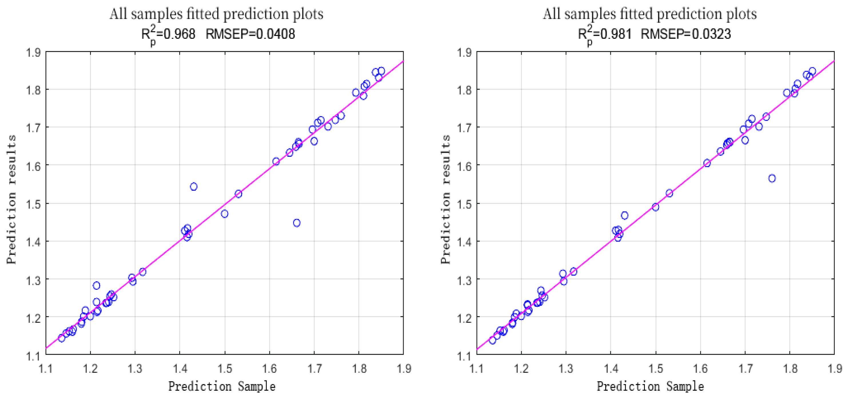
SPA	RIME-LS-SVM	0.9955	0.9404	0.0179	0.0637
CARS-PLS	RIME-LS-SVM	0.998	0.964	0.0126	0.052

).

3.2.2. Inverse Modeling Based on Long- and Short-Term Memory Networks

When the reflectance values of the 47-feature wavelengths screened using the SPA algorithm were used as inputs to construct the LSTM inversion model, an R-squared of 0.6506 and an RMSE of 0.1441 were obtained on the training set, while an R-squared of 0.3307 and an RMSE of 0.2097 were obtained on the test set (Table 1 and Figure 6). When the inversion model was constructed using the reflectance values of 18-feature wavelengths screened using the CARS-PLS algorithm as inputs, an R-squared of 0.7862 and an RMSE of 0.0033 were obtained on the training set, while an R-squared of 0.6155 and an RMSE of 0.0041 were obtained on the test set (Table 1 and Figure 6).

3.2.3. Inverse Modeling Based on Support Vector Regression

When the reflectance values of the 47-feature wavelengths screened using the SPA algorithm were used as inputs to construct the SVR inversion model, an R-squared of 0.9238 and an RMSE of 0.0672 were obtained on the training set, while an R-squared of 0.4966 and an RMSE of 0.1979 were obtained on the test set (Table 1 and Figure 7). When the inversion model was constructed using the reflectance values of the 18 wavelengths screened using the CARS-PLS algorithm as inputs, an R-squared of 0.9306 and an RMSE of 0.0006 were obtained on the training set while, on the test set, an R-squared of 0.7468 and an RMSE of 0.0014 were obtained (Table 1 and Figure 7).

3.2.4. Inverse Modeling Based on the RIME Optimization Algorithm Based on Least Squares Support Vector Machine Regression

It can be seen that, when the RIME-LSSVM inversion model was constructed by using the reflectance values of the 47-feature wavelengths screened using the SPA algorithm as inputs, an R-squared of 0.9955 and an RMSE of 0.0179 were obtained for the training set while, for the test set, an R-squared of 0.9404 and an RMSE of 0.0637 were obtained (Table 1 and Figure 8). When the inversion model was constructed using the reflectance values of the 18-feature wavelengths screened using the CARS-PLS algorithm as inputs, an R-squared of 0.998 and an RMSE of 0.0126 were obtained for the training set while, for the test set, an R-squared of 0.964 and an RMSE of 0.052 were obtained (Table 1 and Figure 8).

The prediction results based on the RIME-LSSVM model for all feature band samples extracted via the SPA algorithm and the CARS-PLS algorithm show that the R-squared of the prediction results for all feature band samples extracted using the SPA algorithm is 0.968 and the RMSE is 0.0408 (Figure 9). Meanwhile, the prediction result for all samples from the feature bands extracted using the CARS-PLS algorithm had an R-squared of 0.981 and an RMSE of 0.0323 (Figure 9). Therefore, the accuracy of the inversion model constructed based on the reflectance values of the feature wavelengths screened using the CARS-PLS algorithm was higher than that of the model using the SPA algorithm.

4. Discussion

Nitrogen is an essential element for plant growth and development. As a key component of important macromolecules, especially in the pre-growth period of fruit trees, adequate nitrogen application determines yield and fruit quality. Alva et al. [41] took “Valencia”, “Parson Brown”, “Hamlin”, and “Sunburst” as experimental materials to explore the effects of different nitrogen application conditions on nitrogen accumulation and fruit growth and development during the growth period. Their results showed a rapid increase in cumulative nitrogen values and a rapid increase in fruit weight and diameter in June, August, and September, and a slow increase in the rest of the reproductive period, indicating the importance of adequate nitrogen supply for fruit and quality at the initial stages of fruit development and growth. Consequently, measuring the nitrogen content by means of inversion can provide a more comprehensive and rapid understanding of the nutritional status and growth condition of apples.

At present, in the study of an inverse model construction of crop physiological growth indicators using hyperspectral reflectance data, it was found that the model accuracy obtained by directly utilizing the original hyperspectral reflectance for inverse model construction of crop physiological growth indicators is often relatively low. This is due to the susceptibility of canopy spectra to crop structural characteristics, light intensity, and anthropogenic disturbances. Previous studies have shown [42] that preprocessing of spectral data can eliminate spectral noise, enhance spectral properties, and improve model accuracy. For example, Jayaselan et al. [43] performed nutrient prediction for palm oil and developed a PLS prediction model after preprocessing the spectral data with MSC, first and second derivatives and standard normal variation (SNV), Gaussian filtering, and SG smoothing, respectively. The results show that the highest model accuracy is obtained after MSC preprocessing with a predicted R-squared of 0.91, and the preprocessing of spectral data can effectively improve the model accuracy. In this study, the raw hyperspectral data were preprocessed with SG smoothing and MSC.

For this study, we constructed a variety of apple canopy leaf hyperspectral nitrogen inversion models for the different fertility stages of apples. Because modeling using the full band suffers from data redundancy and low model accuracy, in order to reduce the data dimension, redundant information and noise should be removed, the estimation model accuracy should be improved, and saturation should be avoided. The CARS-PLS and SPA methods were used to screen the spectral data from the full-band spectral data, and the sensitive bands were extracted as input values to construct the nitrogen inversion model by combining three different algorithms. Among them, the CARS-PLS algorithm extracted 18 sensitive bands, mainly in the range of 750~1032 nm. Studies have shown that nitrogen affects photosynthesis during crop growth, which in turn affects the absorption of blue and red light by the crop, which is in line with previous findings [44,45]. The feature bands screened by CARS-PLS were fewer than those screened by SPA. The R-squared of the accuracy of the nitrogen content estimation models constructed by CARS-PLS were 0.6155, 0.7468, and 0.964, respectively; and the RMSE values were 0.0041, 0.0014, and 0.052, which were higher than those of the models constructed using the feature bands screened by SPA and consistent with the results of [32,46]. The reason may be due to the fact that SPA mainly examines individual spectral bands in the process of screening the characteristic bands and does not take into account the synergistic effect of the combination of spectral bands. And CARS-PLS obtains the optimal subset of variables through the adaptive weighted sampling method and the exponential decay function, which can not only cause the effect of covariance between spectral bands to be effectively reduced and eliminate redundant information in spectral data, but also take into account the synergistic effect between filtered bands.

Comparing the inversion models constructed by the three different algorithms, the results show that the CARS-PLS-RIME-LSSVM model has a higher accuracy than the CARS-PLS-LSTM and CARS-PLS-SVR models due to the fact that the RIME-LSSVM model can better process the data and is more robust to parameter selection, while the SVR modeling accuracy is better than that of the LSTM. This is due to the better generalization ability of the SVR model. However, the spectral eigen-band modeling methods still have shortcomings, and the RIME algorithm has much room for improvement. In future work, the method proposed in this paper will be combined with the vegetation index for more in-depth research, which will provide a method for realizing a more accurate inversion of the nitrogen content of apple canopy leaves.

5. Conclusions

In this study, after preprocessing the raw spectral data using SG-MSC, the feature bands were screened using the CARS-PLS and SPA algorithms to construct a prediction model for nitrogen content. The R-squared value of the training set of the RIME-LSSVM model was improved by 0.2117 and that of the test set was improved by 0.3486 when compared to the long- and short-term memory network. Similarly, with the RIME-LSSVM model, the R-squared value of the training set increased by 0.0673 and the R-squared value of the test set increased by 0.2172 compared to the support vector regression model. Therefore, among the three nonlinear models, the RIME-LSSVM model is the most accurate. A method is provided to quickly obtain the nitrogen content of apple tree leaves.

References

- Qu, Z.; Zhou, G. Possible impact of climate change on the quality of apples from the major producing areas of China. Atmosphere 2016, 7, 113. [Google Scholar] [CrossRef]
- Cao, H.; Wang, H.; Li, Y.; Hamani, A.K.M.; Zhang, N.; Wang, X.; Gao, Y. Evapotranspiration partition and dual crop coefficients in apple orchard with dwarf stocks and dense planting in arid region, Aksu oasis, southern Xinjiang. Agriculture 2021, 11, 1167. [Google Scholar] [CrossRef]
- Colpaert, B.; Steppe, K.; Gomand, A.; Vanhoutte, B.; Remy, S.; Boeckx, P. Experimental approach to assess fertilizer nitrogen use, distribution, and loss in pear fruit trees. Plant Physiol. Biochem. 2021, 165, 207–216. [Google Scholar] [CrossRef] [PubMed]
- Poudel, D.D.; Horwath, W.R.; Mitchell, J.P.; Temple, S.R. Impacts of cropping systems on soil nitrogen storage and loss. Agric. Syst. 2001, 68, 253–268. [Google Scholar] [CrossRef]
- Wrona, D. The influence of nitrogen fertilization on growth, yield and fruit size of ‘Jonagored’apple trees. Acta Sci. Pol. Hortorum Cultus 2011, 10, 3–10. [Google Scholar]
- Anjaneyulu, T.S.R. Formaldehyde Titration Method for the Determination of Ammoniacal Nitrogen in Phosphate Fertilizers. J. Assoc. Off. Anal. Chem. 1975, 58, 1194–1196. [Google Scholar] [CrossRef]
- Sharifi, M.; Zebarth, B.J.; Burton, D.L.; Grant, C.A.; Hajabbasi, M.A.; Abbassi-Kalo, G. Sodium hydroxide direct distillation: A method for estimating total nitrogen in soil. Commun. Soil Sci. Plant Anal. 2009, 40, 2505–2520. [Google Scholar] [CrossRef]
- Ulissi, V.; Antonucci, F.; Benincasa, P.; Farneselli, M.; Tosti, G.; Guiducci, M.; Tei, F.; Costa, C.; Pallottino, F.; Pari, L. Nitrogen concentration estimation in tomato leaves by VIS-NIR non-destructive spectroscopy. Sensors 2011, 11, 6411–6424. [Google Scholar] [CrossRef]
- Wang, J.; Shen, C.; Liu, N.; Jin, X.; Fan, X.; Dong, C.; Xu, Y. Non-destructive evaluation of the leaf nitrogen concentration by in-field visible/near-infrared spectroscopy in pear orchards. Sensors 2017, 17, 538. [Google Scholar] [CrossRef]
- Ma, J.; Cheng, J.; Wang, J.; Pan, R.; He, F.; Yan, L.; Xiao, J. Rapid detection of total nitrogen content in soil based on hyperspectral technology. Inf. Process. Agric. 2022, 9, 566–574. [Google Scholar] [CrossRef]
- Yuan, Z.; Ye, Y.; Wei, L.; Yang, X.; Huang, C. Study on the optimization of hyperspectral characteristic bands combined with monitoring and visualization of pepper leaf SPAD value. Sensors 2021, 22, 183. [Google Scholar] [CrossRef]
- Chen, X.; Lv, X.; Ma, L.; Chen, A.; Zhang, Q.; Zhang, Z. Optimization and Validation of Hyperspectral Estimation Capability of Cotton Leaf Nitrogen Based on SPA and RF. Remote Sens. 2022, 14, 5201. [Google Scholar] [CrossRef]
- Hu, L.; Yin, C.; Ma, S.; Liu, Z. Rapid detection of three quality parameters and classification of wine based on Vis-NIR spectroscopy with wavelength selection by ACO and CARS algorithms. Spectrochim. Acta Part A Mol. Biomol. Spectrosc. 2018, 205, 574–581. [Google Scholar] [CrossRef] [PubMed]
- Heylen, R.; Parente, M.; Gader, P. A review of nonlinear hyperspectral unmixing methods. IEEE J. Sel. Top. Appl. Earth Obs. Remote Sens. 2014, 7, 1844–1868. [Google Scholar] [CrossRef]
- Miphokasap, P.; Wannasiri, W. Estimations of nitrogen concentration in sugarcane using hyperspectral imagery. Sustainability 2018, 10, 1266. [Google Scholar] [CrossRef]
- Silva, R.; Gomes, V.; Mendes-Faia, A.; Melo-Pinto, P. Using support vector regression and hyperspectral imaging for the prediction of oenological parameters on different vintages and varieties of wine grape berries. Remote Sens. 2018, 10, 312. [Google Scholar] [CrossRef]
- Khan, A.; Vibhute, A.D.; Mali, S.; Patil, C.H. A systematic review on hyperspectral imaging technology with a machine and deep learning methodology for agricultural applications. Ecol. Inform. 2022, 69, 101678. [Google Scholar] [CrossRef]
- Wang, F.; Huang, J.; Wang, Y.; Liu, Z.; Zhang, F. Estimating nitrogen concentration in rape from hyperspectral data at canopy level using support vector machines. Precis. Agric. 2013, 14, 172–183. [Google Scholar] [CrossRef]
- Bruning, B.; Liu, H.; Brien, C.; Berger, B.; Lewis, M.; Garnett, T. The development of hyperspectral distribution maps to predict the content and distribution of nitrogen and water in wheat (Triticum aestivum). Front. Plant Sci. 2019, 10, 1380. [Google Scholar] [CrossRef]
- Guo, J.; Zhang, J.; Xiong, S.; Zhang, Z.; Wei, Q.; Zhang, W.; Feng, W.; Ma, X. Hyperspectral assessment of leaf nitrogen accumulation for winter wheat using different regression modeling. Precis. Agric. 2021, 22, 1634–1658. [Google Scholar] [CrossRef]
- Yu, F.; Feng, S.; Du, W.; Wang, D.; Guo, Z.; Xing, S.; Jin, Z.; Cao, Y.; Xu, T. A study of nitrogen deficiency inversion in rice leaves based on the hyperspectral reflectance differential. Front. Plant Sci. 2020, 11, 573272. [Google Scholar] [CrossRef]
- Azadnia, R.; Rajabipour, A.; Jamshidi, B.; Omid, M. New approach for rapid estimation of leaf nitrogen, phosphorus, and potassium contents in apple-trees using Vis/NIR spectroscopy based on wavelength selection coupled with machine learning. Comput. Electron. Agric. 2023, 207, 107746. [Google Scholar] [CrossRef]
- Gómez-Casero, M.T.; López-Granados, F.; Pena-Barragán, J.M.; Jurado-Expósito, M.; García-Torres, L.; Fernández-Escobar, R. Assessing nitrogen and potassium deficiencies in olive orchards through discriminant analysis of hyperspectral data. J. Am. Soc. Hortic. Sci. 2007, 132, 611–618. [Google Scholar] [CrossRef]
- Somers, B.; Delalieux, S.; Verstraeten, W.W.; Eynde, A.V.; Barry, G.H.; Coppin, P. The contribution of the fruit component to the hyperspectral citrus canopy signal. Photogramm. Eng. Remote Sens. 2010, 76, 37–47. [Google Scholar] [CrossRef]
- Einzmann, K.; Atzberger, C.; Pinnel, N.; Glas, C.; Böck, S.; Seitz, R.; Immitzer, M. Early detection of spruce vitality loss with hyperspectral data: Results of an experimental study in Bavaria, Germany. Remote Sens. Environ. 2021, 266, 112676. [Google Scholar] [CrossRef]
- Jaroonchon, N.; Krisanapook, K.; Phavaphutanon, L. Correlation between pummelo leaf nitrogen concentrations determined by combustion method and Kjeldahl method and their relationship with SPAD values from portable chlorophyll meter. Agric. Nat. Resour. 2010, 44, 800–807. [Google Scholar]
- Kale, K.V.; Solankar, M.M.; Nalawade, D.B.; Dhumal, R.K.; Gite, H.R. A research review on hyperspectral data processing and analysis algorithms. Proc. Natl. Acad. Sci. India Sect. A Phys. Sci. 2017, 87, 541–555. [Google Scholar] [CrossRef]
- Yang, X.; Hong, H.; You, Z.; Cheng, F. Spectral and image integrated analysis of hyperspectral data for waxy corn seed variety classification. Sensors 2015, 15, 15578–15594. [Google Scholar] [CrossRef] [PubMed]
- Yu, Y.; Yu, H.; Guo, L.; Li, J.; Chu, Y.; Tang, Y.; Tang, S.; Wang, F. Accuracy and stability improvement in detecting Wuchang rice adulteration by piece-wise multiplicative scatter correction in the hyperspectral imaging system. Anal. Methods 2018, 10, 3224–3231. [Google Scholar] [CrossRef]
- Wei, X.; He, J.; Zheng, S.; Ye, D. Modeling for SSC and firmness detection of persimmon based on NIR hyperspectral imaging by sample partitioning and variables selection. Infrared Phys. Technol. 2020, 105, 103099. [Google Scholar] [CrossRef]
- Khan, I.H.; Liu, H.; Cheng, T.; Tian, Y.; Cao, Q.; Zhu, Y.; Cao, W.; Yao, X. Detection of wheat powdery mildew based on hyperspectral reflectance through SPA and PLS-LDA. Int. J. Precis. Agric. Aviat. 2020, 3, 13–22. [Google Scholar] [CrossRef]
- Sun, J.; Ma, B.; Dong, J.; Zhu, R.; Zhang, R.; Jiang, W. Detection of internal qualities of hami melons using hyperspectral imaging technology based on variable selection algorithms. J. Food Process Eng. 2017, 40, e12496. [Google Scholar] [CrossRef]
- Zhang, D.; Xu, Y.; Huang, W.; Tian, X.; Xia, Y.; Xu, L.; Fan, S. Nondestructive measurement of soluble solids content in apple using near infrared hyperspectral imaging coupled with wavelength selection algorithm. Infrared Phys. Technol. 2019, 98, 297–304. [Google Scholar] [CrossRef]
- Sherstinsky, A. Fundamentals of recurrent neural network (RNN) and long short-term memory (LSTM) network. Phys. D Nonlinear Phenom. 2020, 404, 132306. [Google Scholar] [CrossRef]
- Shewalkar, A.; Nyavanandi, D.; Ludwig, S.A. Performance evaluation of deep neural networks applied to speech recognition: RNN, LSTM and GRU. J. Artif. Intell. Soft Comput. Res. 2019, 9, 235–245. [Google Scholar] [CrossRef]
- Farzad, A.; Mashayekhi, H.; Hassanpour, H. A comparative performance analysis of different activation functions in LSTM networks for classification. Neural Comput. Appl. 2019, 31, 2507–2521. [Google Scholar] [CrossRef]
- Huang, S.; Cai, N.; Pacheco, P.P.; Narrandes, S.; Wang, Y.; Xu, W. Applications of support vector machine (SVM) learning in cancer genomics. Cancer Genom. Proteom. 2018, 15, 41–51. [Google Scholar]
- Awad, M.; Khanna, R.; Awad, M.; Khanna, R. Support vector regression. In Efficient Learning Machines: Theories, Concepts, and Applications for Engineers and System Designers; Apress: New York, NY, USA, 2015; pp. 67–80. [Google Scholar]
- Suykens, J.A.; Lukas, L.; Van Dooren, P.; De Moor, B.; Vandewalle, J. Least squares support vector machine classifiers: A large scale algorithm. In Proceedings of the European Conference on Circuit Theory and Design, ECCTD, Stresa, Italy, 29 August–2 September 1999; pp. 839–842. [Google Scholar]
- Su, H.; Zhao, D.; Heidari, A.A.; Liu, L.; Zhang, X.; Mafarja, M.; Chen, H. RIME: A physics-based optimization. Neurocomputing 2023, 532, 183–214. [Google Scholar] [CrossRef]
- Alva, A.K.; Paramasivam, S.; Hostler, K.H.; Easterwood, G.W.; Southwell, J.E. Effects of nitrogen rates on dry matter and nitrogen accumulation in citrus fruits and fruit yield. J. Plant Nutr. 2001, 24, 561–572. [Google Scholar] [CrossRef]
- Hunt, E.R., Jr.; Doraiswamy, P.C.; McMurtrey, J.E.; Daughtry, C.S.; Perry, E.M.; Akhmedov, B. A visible band index for remote sensing leaf chlorophyll content at the canopy scale. Int. J. Appl. Earth Obs. Geoinf. 2013, 21, 103–112. [Google Scholar] [CrossRef]
- Jayaselan, H.A.J.; Ismail, W.I.W.; Nawi, N.M.; Shariff, A.R.M. Determination of the Optimal Pre-processing Technique for Spectral Data of Oil Palm Leaves with Respect to Nutrient. Pertanika J. Sci. Technol. 2018, 26, 1169–1182. [Google Scholar]
- Shu, M.; Shen, M.; Zuo, J.; Yin, P.; Wang, M.; Xie, Z.; Tang, J.; Wang, R.; Li, B.; Yang, X. The application of UAV-based hyperspectral imaging to estimate crop traits in maize inbred lines. Plant Phenomics 2021, 2021, 9890745. [Google Scholar] [CrossRef]
- Mishra, G.; Panda, B.K.; Ramirez, W.A.; Jung, H.; Singh, C.B.; Lee, S.H.; Lee, I. Research advancements in optical imaging and spectroscopic techniques for nondestructive detection of mold infection and mycotoxins in cereal grains and nuts. Compr. Rev. Food Sci. Food Saf. 2021, 20, 4612–4651. [Google Scholar] [CrossRef]
- Hong, G.; Abd El-Hamid, H.T. Hyperspectral imaging using multivariate analysis for simulation and prediction of agricultural crops in Ningxia, China. Comput. Electron. Agric. 2020, 172, 105355. [Google Scholar] [CrossRef]