Article

Automatic Separation of Photosynthetic Components in a LiDAR Point Cloud Data Collected from a Canadian Boreal Forest

by
Leila Taheriazad
1,
Hamid Moghadas
2 and
Arturo Sanchez Azofeifa
1,*
1
Department of Earth and Atmospheric Sciences, University of Alberta, Edmonton, AB T6G 2E3, Canada
2
Department of Mechanical Engineering, University of Alberta, Edmonton, AB T6G 1H9, Canada
*
Author to whom correspondence should be addressed.
Forests 2024, 15(1), 70; https://doi.org/10.3390/f15010070
Submission received: 24 November 2023 / Revised: 18 December 2023 / Accepted: 22 December 2023 / Published: 29 December 2023
(This article belongs to the Section Forest Inventory, Modeling and Remote Sensing)

Abstract

:
Terrestrial LiDAR has emerged as a promising technology for accurate forest assessment. LiDAR can provide a 3D image composed of a cloud of points using a rotary laser scanner. The point cloud data (PCD) contain information on the (x, y, z) coordinates of every single scanned point and a raw intensity parameter. This study introduces an algorithm for the automatic and accurate separation of the photosynthetic features of a PCD. It is shown that the recorded raw intensity is not a suitable parameter for the separation of photosynthetic features. Instead, for the first time, the absorption intensity is developed for every point based on its raw intensity and distance from the scanner, using proper scaling functions. Then, the absorption intensity is utilized as the only criterion for the classification of the points between photosynthetic and non-photosynthetic features. The proposed method is applied to the scans from a Canadian Boreal Forest and successfully extracted the photosynthetic features with minimal average type I and type II error rates of 5.7% and 4.8%. The extracted photosynthetic PCD can be readily used for calculating important forest parameters such as the leaf area index (LAI) and the green biomass. In addition, it can be used for estimating forest carbon storage and monitoring temporal changes in vegetation structure and ecosystem health.

1. Introduction

The evaluation of the canopy structure is crucial for sustainable forest management, ecosystem function modeling, and global ecosystem interactions [1,2]. Separating leaves from wood in terrestrial laser scanning (TLS) data is important in various ecological applications, such as radiation transfer modeling, energy and mass exchange, and analysis of the net primary production for different tree components [3,4]. It is particularly important to include a leaf filter in the classification of tree species as deciduous trees undergo seasonal foliage changes, which can limit classification generalizability [5].
Light detection and ranging (LiDAR) and TLS are remote sensing technologies that provide suitable tools for analyzing the structure of forest canopies and estimating their biophysical parameters [1,2,3,4]. Terrestrial LiDAR, a ground-based LiDAR system, emits laser pulses to capture three-dimensional coordinate information of objects in its target area [6]. This technology can generate dense point clouds quickly and accurately, which sets it apart from other measurement methods and makes it a suitable technology for collecting detailed and dense 3D point clouds of trees [7]. LiDAR, including TLS, provides a high-resolution platform for acquiring 3D point cloud data, making it one of the most advanced remote sensing systems available [6,7].
TLS has become increasingly popular in the field of forest ecosystem science over the past few decades. This technology, which generates high-resolution 3D point clouds, has proven to be useful for a wide range of applications such as modeling branch architecture (as demonstrated by Lau et al. 2018 and Zhang et al. 2022) [8,9], conducting forest field inventory [7], measuring fuel hazards [10], and assessing habitat conditions [11]. TLS allows for precise and detailed data collection, making it an appropriate tool for accurate and reliable analysis in various ecological contexts. Prior to performing tree architecture modeling and estimating biophysical parameters, it is necessary to separate the wood and leaf components, as accurate estimations of parameters like the leaf area index (LAI) require precise leaf and wood separation. The LAI has been considered one of the primary variables in forest ecology science [12], and mixed wood may lead to an overestimation of the LAI. The LiDAR captures a heterogeneous mixture of forest features, such as wood and leaf, which results in PCD that require further analysis. Several studies have focused on extracting leaf and wood from the PCD [13,14,15,16,17,18,19,20,21,22,23,24,25,26]. This task is particularly challenging due to the irregular distribution and intermingling of millions of points representing leaf and wood within a single tree.
To address the challenge of separating leaf and wood points, some studies have opted to calculate the plant area index (PAI) as an alternative to the LAI [27,28,29]. However, the PAI is not a suitable approximation of the LAI as it considers the entire PCD, including wood points. Woody materials have been identified as a major source of error in LAI estimation [30,31,32]. Hosoi and Omasa (2007) [33] discovered that depending on the tree canopy, errors in estimating the LAI can range from 4.2% to 32.7% due to woody materials. Clawges et al. (2007) [34] found that woody material can account for 24% to 58% of the total area of a tree. In a study conducted by Moorthy et al. (2008) [35], the initial estimation of PAI with the inclusion of woody material improved LAI retrievals, resulting in a lower root-mean-square error (RMSE) of 0.68, as opposed to a RMSE of 1.13 without including woody material. Thus, it is essential to separate woody material from leaf to achieve accurate LAI assessment. As a result, some studies have calculated the total biomass instead of green biomass [36].
While many TLS methods in ecology are promising, separating wood and leaf in point clouds remains challenging. This issue is crucial for the reliability and precision of these methods [25,37,38]. Methods for separating data in TLS can be grouped based on their main approach. These include using the geometry of points, such as their location and closeness, the intensity of the points that are returned, or a mix of both these methods [3].
Three techniques have been proposed for separating photosynthetic and non-photosynthetic materials in tree PCD. The first method involves manual separation by the operator using visual color-based recognition and the geometrical distribution of points, with the assistance of a 3D demonstration software [39,40,41,42]. However, this technique is time-consuming and prone to user error due to the large number of scattered points forming various geometries. As a result, alternative automated techniques have been developed. The second approach employs statistical tools like eigenvalues, conditional probability functions, and Gaussian mixture models to identify leaf geometry [26,43,44,45,46,47,48]. A potential drawback of the geometry identification method is that the LiDAR scanning process may undersample many leaves, resulting in only a few points representing them. Recently, an alternative method has been proposed that utilizes point “intensity” to identify photosynthetic material from non-photosynthetic material [2,49,50,51,52,53]. Point intensity is a measurement provided using the LiDAR in addition to the Cartesian coordinates of a point (x, y, z). It is defined based on the amount of laser beam reflection received at the LiDAR scanner, influenced by various factors such as the material composition of the hit point, laser wavelength, incidence angle, and distance between the laser scanner and the hit point [54].
Each of the aforementioned factors needs to be studied individually. Firstly, the constituent materials of the hit point should be considered, as the absorption of laser beam energy by leaves, with their higher chlorophyll and water content, differs significantly from wood material [2,26,55,56,57,58]. Secondly, the laser wavelength is an important factor that is determined using the laser transceiver. While some LiDAR systems use a single wavelength, others utilize multiple wavelengths to provide more information about hit point features, resulting in a higher cost of the apparatus [59,60]. The Leica C10, which is the instrument used in this study, operates with a single wavelength of 532 nm (green light). Thirdly, the incidence angle of a laser beam is dependent on the orientation of the beam relative to the extent of the leaf or wood. Lastly, the distance between the source and the hit point affects the power of the laser beam, which is inversely proportional to the squared distance [54], thereby limiting the range of distance supported by each LiDAR instrument depending on the sensitivity of its receiver [61]. For the Leica C10, the maximum distance supported is 300 m [62]. The techniques utilized in previous studies [2,49,50,51,52,53,63] that rely on raw intensity for distinguishing between leaf and wood points do not account for the effects of two independent factors: constituent materials and distance from the scanner. As the points that constitute tree PCD are situated at varying distances from the scanning station, raw intensity is not an appropriate attribute for separating leaf and wood.
This study presents an algorithm for the automatic and accurate separation of photosynthetic features in LiDAR PCD. It is verified that the recorded raw intensity is not a suitable parameter for the classification task. Hereby, for the first time, the absorption intensity is developed based on LiDAR data. For calculating the absorption intensity, the raw intensity was rescaled and multiplied by the squared distance between the scan station and the hit point on the tree. The absorption intensity is utilized as the only criterion for the classification of the points between photosynthetic and non-photosynthetic components. The proposed algorithm is applied to the scans from a Canadian Boreal Forest and successfully extracted the photosynthetic components with minimal average type I and type II error rates of 5.7% and 4.8%.
The proposed method has several advantages over the current methods in the literature. Firstly, the LiDAR PCD are sufficient for it. Standard calibration panels [2,53] or other scanners are not needed. Secondly, the algorithm does not need information on the tree species or the forest type. Thirdly, the classification criterion is a single parameter, absorption intensity, and the classification task is a single rule (absorption intensity > optimum threshold intensity). Hence, the computational load is not heavy. The dominant algorithms in the literature have several parameters that strongly affect the classification performance and should be fine-tuned for every single tree. Fourthly, since the local point density in PCD and the geometry of the leaf, branch, and trunk are not considered in our algorithm, under-sampled components will be classified correctly. Undersampling occurs in laser scanning due to occlusion, high forest density, or using a low number of scan stations. In our proposed method, every single point in PCD is tested and classified individually and independently from other points in its neighborhood.

2. Materials and Methods

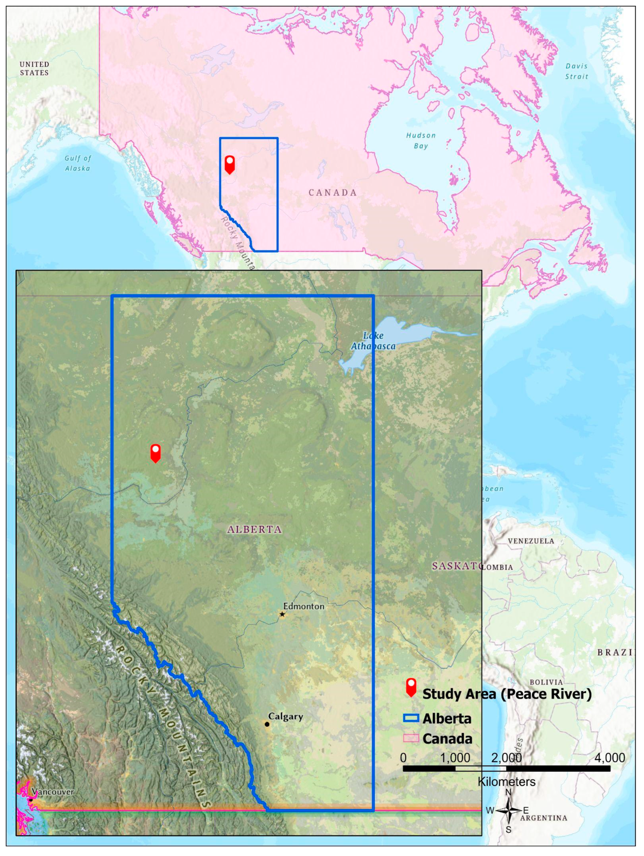
2.1. Study Area and Site Characteristics

In the Peace River Environmental Monitoring Super Site (PR-EMSS), a rectangular study plot measuring 50 m × 50 m was established within a Trembling Aspen (Populus tremuloides) forest stand characterized by a broad leaf deciduous canopy. The survey was conducted between August and October of 2014 in an undulating terrain situated at latitude 56°44′39″ North and longitude −118°20′40″ West, with an elevation of 871 m (Figure 1). For all trees within the plot, both the tree height and diameter at breast height (DBH) were collected utilizing a TruPulse 200 laser rangefinder and a measuring tape.

2.2. Instrument and In Situ Measurements Description

The terrestrial laser scanning system utilized in this study was the Leica Scan Station C10 manufactured by Leica Geosystems AG, Heerbrugg, Switzerland. The Leica Scan Station C10 emitted laser beam pulses at 532 nm (green laser) within a field of view window of 360° × 270°. As is typical in studies focusing on the separation of wood and leaf, specific instructions, equations, and curves were developed based on the laser apparatus’ wavelength. The Leica C10 is a discrete return LiDAR, meaning that it only employs the first return points to characterize the object at a particular location. The information obtained from the Leica C10 includes coordinate data (x, y, z) and intensity, and the system uses the beam’s travel time to calculate the distance to targets. For a target with a 90% albedo, the instrument can detect a return signal from up to 300 m away, while for an 18% albedo target, the maximum range is 134 m. The Leica C10 is also capable of capturing data from short-range targets with a minimum distance of approximately 0.1 m. Notably, the PCD obtained from the Leica C10 scanner do not provide information on the surface vectors of either leaf or wood. This factor is disregarded in the current study, as well as in the current state-of-the-art literature, under the assumption of Lambertian scattering.
It should be emphasized that the Leica C10 scanner’s PCD do not include data on the surface vectors of leaf or wood. This factor has been overlooked in both current research and in the literature, assuming Lambertian scattering. The assumption of Lambertian scattering, which neglects the surface vectors of leaf and wood, is commonly made in studies that use terrestrial laser scanning to estimate forest structure and biomass [64,65,66,67]. It is worth noting that while the assumption of Lambertian scattering simplifies the modeling of light interaction with surfaces, it may introduce errors in the estimation of forest structure and biomass, particularly in areas with complex topography or with non-Lambertian surfaces. Several studies have explored the impact of non-Lambertian surface effects on terrestrial laser scanning measurements and have proposed methods to account for them [68,69].
To mitigate the occlusion effect, the trees under investigation were scanned from six different locations. The scanning was conducted during both the leaf on-season (summer 2014) and leaf off-season (fall 2014) at identical locations in both seasons. The PCD obtained during the leaf off-season, when there is no foliage, were employed as a reference to evaluate the separation both qualitatively and quantitatively. This approach allowed us to better understand the performance of the scanning method in capturing the structure of the trees under different conditions and to account for any potential biases or errors that may have been introduced by occlusion effects during the leaf on-season.
To perform the medium-resolution scanning, each scan required approximately 10–15 min to complete. The Leica C10 scanner was positioned on a leveled survey tripod at a height of approximately 1.5 m above the ground to avoid interference from the dense understory. Following the scans, the Cyclone 8.1 software was used to align any pairs of scans to common reference targets. MATLAB Software (R2016b) was utilized for all processing of the LiDAR PCD [70]. The study area had an average tree density of 675 trees per hectare, consisting mainly of mature trees with a diameter at breast height exceeding 5 cm. A subset of Trembling Aspen trees within a 50 m × 50 m plot in the study area was chosen for both LiDAR and field measurements. The proposed method was then applied to a total of 21 trees.

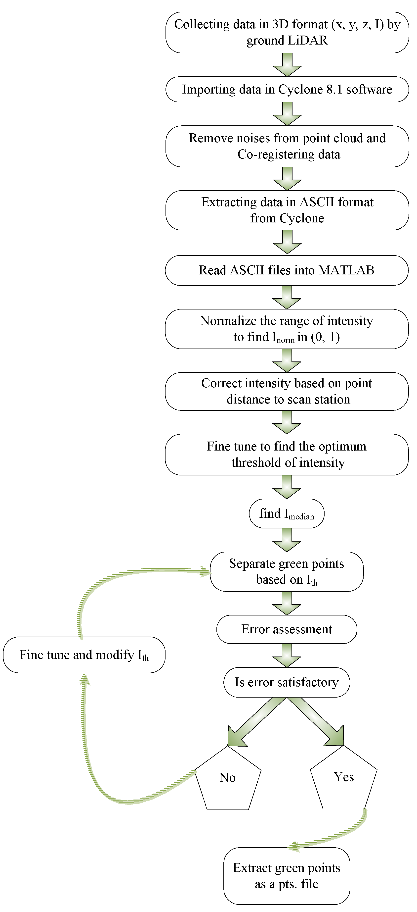
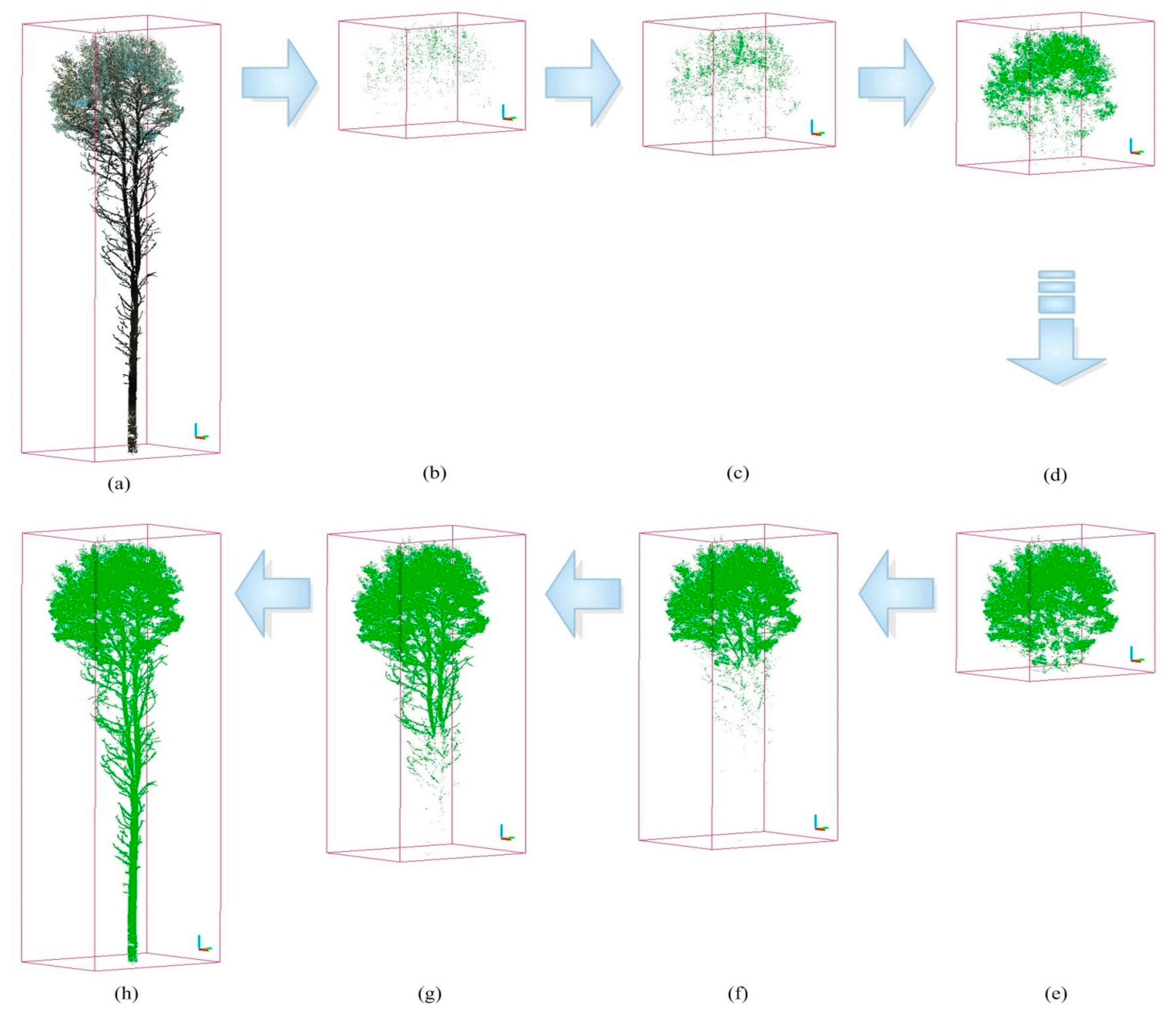
2.3. Algorithm Steps

An algorithm has been developed that can automatically separate photosynthetic from non-photosynthetic components in LiDAR point cloud data. This method does not require any information on temporal characteristics such as seasonal data, laser wavelength, or tree distance. The steps of the algorithm are presented in a summary format in Figure 2 and are explained in further detail in the following sections. The LiDAR PCD data for trees, including point coordinates and intensity (x, y, z, I), obtained during the leaf on season, is fed into the algorithm. The intensity values, denoted by I, are real numbers ranging from −2047 to +2048.
I. To normalize the range of values for the point intensity (I), a scaling operation is performed. The range of values for I, which is (−2047, +2048), is transformed to a scale of (0, +1) using the following equation:
I_norm = (I/4095) + (2048/4095)
II. When the laser beam hits a point and returns to the LiDAR, its intensity depends on the power loss that it undergoes during its travel. This loss is due to path loss and absorption loss, as shown in Figure 3. Path loss is proportional to the squared distance (R2) between the LiDAR and the hit point, which is known for each point in the PCD [54]. The red arrows in Figure 3 illustrate the path loss from the LiDAR to the hit spot on the leaf and from the hit spot to the LiDAR. On the other hand, absorption loss is caused by water, pigment, and surface physical properties, which vary between photosynthetic and non-photosynthetic components. This is shown in Figure 3 by the orange bouncing arrow over the leaf. To distinguish between photosynthetic and non-photosynthetic, we need to isolate the absorption loss from the path loss. To obtain the intensity only due to absorption loss (I_absorption), we multiply I_norm by the squared distance as follows:
I_absorption = I_norm × R2
The distance for each specific point can be calculated using the Cartesian coordinate (x, y, z) recorded using the LiDAR, as shown in Equation (3).
R = √(x2 + y2 + z2).
As a result, the intensity of absorption loss, denoted as I_absorption, can be obtained by multiplying I_norm with the squared distance from the LiDAR to each point in the PCD, which is calculated based on the Cartesian coordinates (x, y, z) provided by the LiDAR device, as shown in Equation (4).
I_absorption = I_norm (x2 + y2 + z2)
III. To differentiate between photosynthetic and non-photosynthetic, it is essential to establish the optimum intensity threshold (OIT) value. Points with an intensity value above the OIT are considered to belong to photosynthetic components with minimal errors. The OIT value determination yields a low and almost identical rate of omission and commission errors, which will be elaborated on in upcoming sections. These two types of errors will be discussed in subsequent sections. The LiDAR point cloud data collected during the leaf off-season (referred to as PCD_r) are used as a reference for evaluating the separated point cloud data. This evaluation allows for the determination of the accuracy and reliability of the algorithm’s ability to differentiate between photosynthetic and non-photosynthetic components of trees. A software program was developed to align and combine the point cloud data that were separated with the reference PCD_r in a three-dimensional space, allowing for point-by-point comparison. The absorption intensity levels are defined within a range between a minimum value (I_min) and a maximum value (I_max).
Five absorption intensity values (I_n) are then uniformly selected from this range using the following equation where n is a value between 1 and 5:
I_n = I_min + n × (I_max − I_min)/6
The algorithm divides the PCD into groups or subsets by utilizing absorption intensity values (I_n) that are evenly distributed and selected within the range of I_min and I_max. For each intensity value, the algorithm separates the points in PCD with an intensity value lower than I_n and puts them into a new subset labeled PCD (I_n). The software program then compares the separated PCD (I_n) with the reference PCD_r collected during the leaf off-season to calculate the rate of omission and commission errors.
IV. The two I_n values with the lowest omission and commission errors were chosen, and Step III was repeated between these two values. This iterative process continues until the two types of error are sufficiently small and closely aligned.
The intensity of the received laser beam from the hit point depends on the total power loss it undergoes during its two-way travel from the laser source to the hit point and back from the hit point to the laser source and target. The path loss is proportional to the squared distance (R2) and is known for every point in the PCD. Path loss is indicated by two red arrows extending from the LiDAR to the hit spot on the leaf and from the hit spot back to the LiDAR, as shown in Figure 3. Absorption loss depends on the water, pigment, and physical properties of the surface. Since leaf and wood tend to have different ranges of water, pigment, and scattering characteristics, absorption loss can be used to identify photosynthetic from non-photosynthetic components. This is indicated by the orange bouncing arrow over the leaf (Figure 3). Absorption loss should be distinguished from path loss to separate the wood from the leaf.

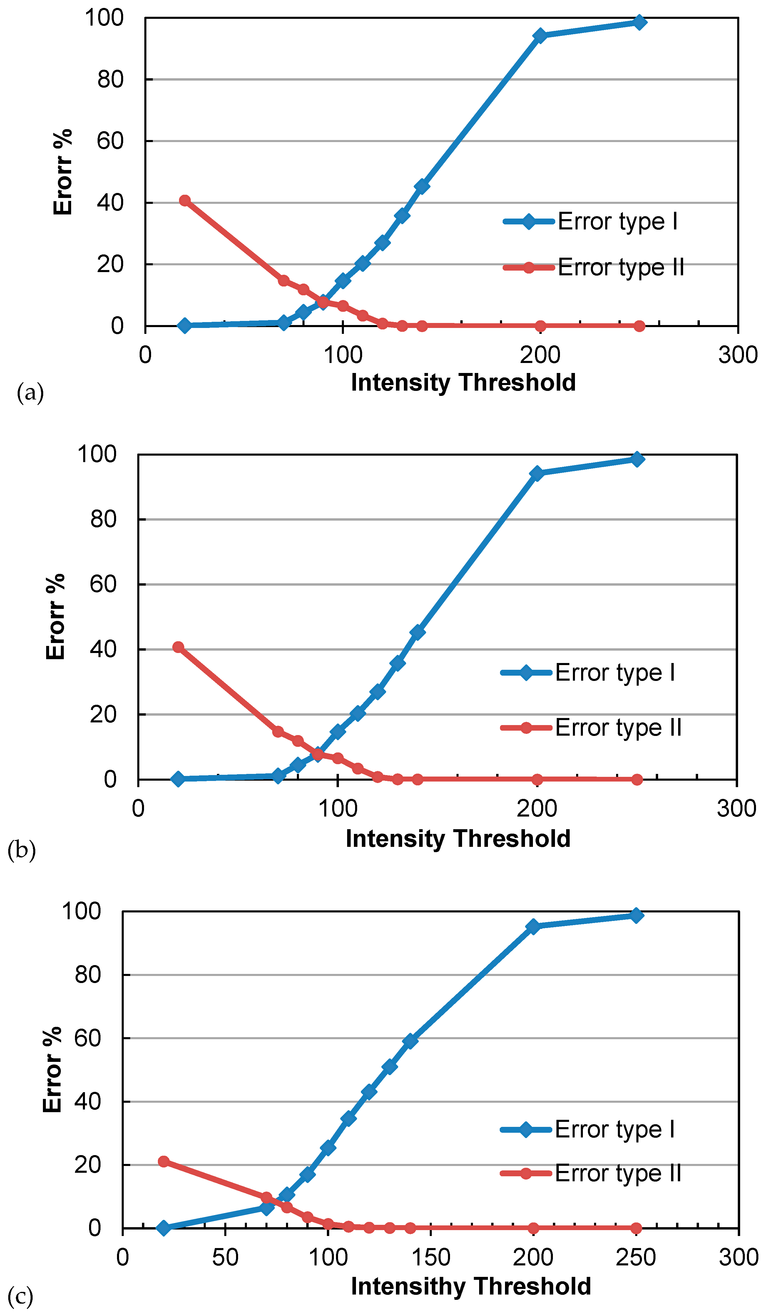
2.4. Accuracy Assessment

The performance of the separation method was assessed using qualitative and quantitative analyses. Qualitative analysis was conducted using 3D PCD demonstration software version 2.6.3 such as Cloud Compare. Both the entire PCD and the separated points were loaded in different colors for visual comparison [70,71,72]. Additionally, the PCD from the leaf off-season were used as a reference for visual comparison with the separated points.
For the quantitative evaluation of the separation method, the Sithole and Vosselman (2004) [72,73] method was utilized. This method involves calculating two types of errors, namely, error type Ι (omission error) and error type ΙΙ (commission error), as expressed in Equation (6):
Error type I = a/GP   
Error type II = b/NGP
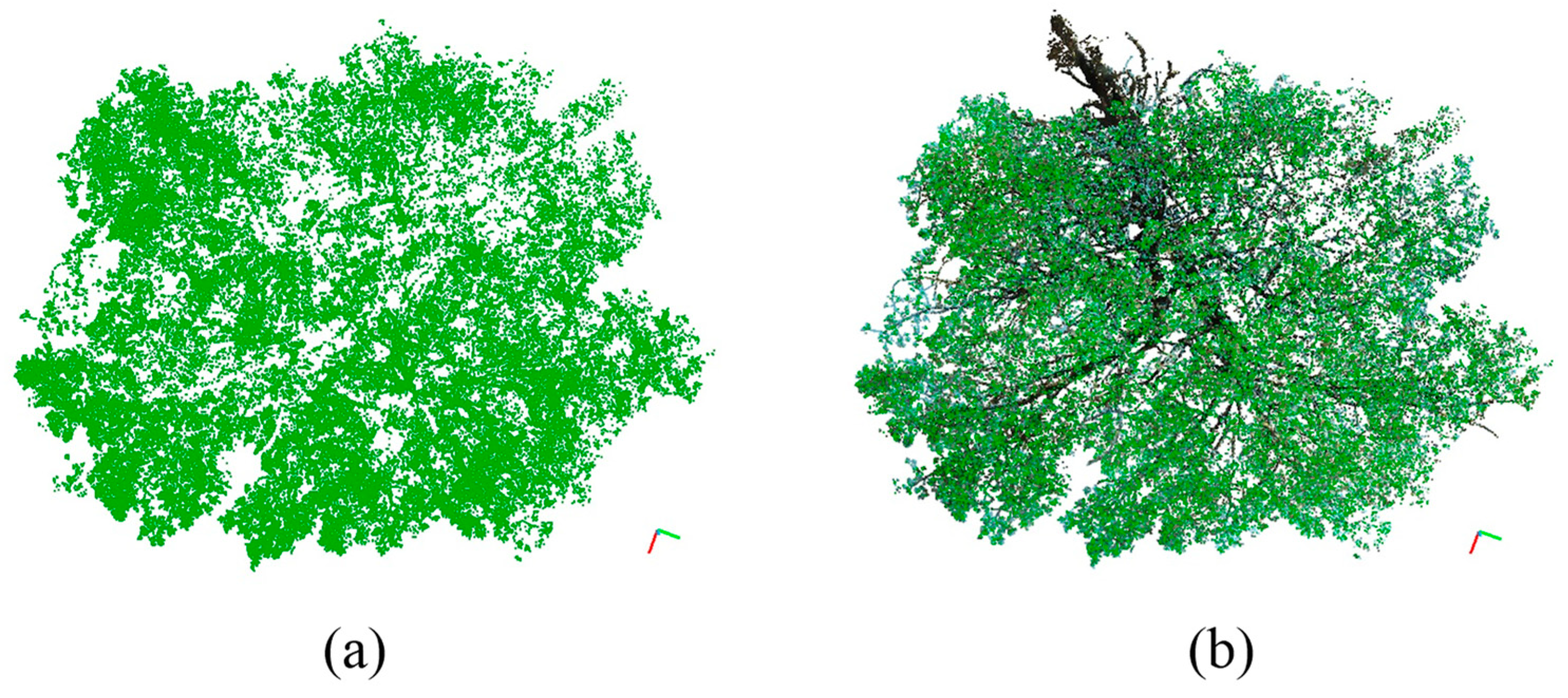
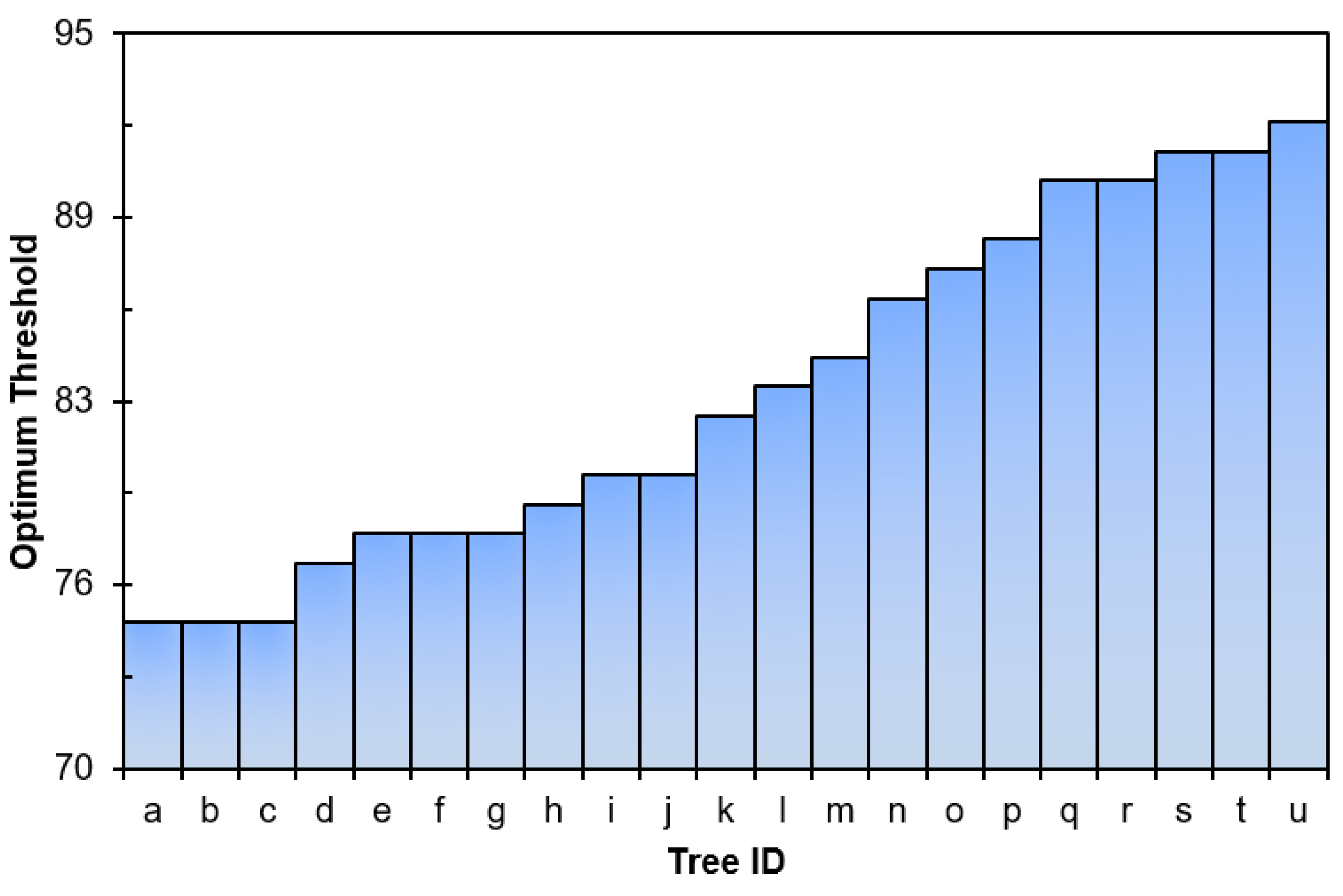
Here, a represents the number of green points erroneously classified as non-green, b represents the number of non-green points incorrectly classified as green, GP is the total count of green points, and NGP is the total count of non-green points during the leaf off-season [73,74]. To count and visualize the different point classes and determine the above parameters, 3D PCD demonstration software, such as Cloud Compare, can be utilized. A computer code written in MATLAB was used to compare the processed PCD with the leaves of PCD and determine the difference between them. The code automatically outputs the number of green and non-green points and, based on these values, calculates the two types of errors: I and II.

3. Results

In this section, the effectiveness of the proposed algorithm in distinguishing between photosynthetic and non-photosynthetic components is evaluated using three PCD of trees during the summer season. The absorption loss varied from 0 to 500, with most values being below 300. The optimal threshold for I_absorption was determined by fine-tuning a range of intensity thresholds, including 250, 200, 90, 86, 70, 50, and 20, as shown in Figure 4. The OIT was then determined by minimizing the commission and omission errors using the proposed algorithm over 21 trees. The average error rates for the type I and type II errors were 5.7% and 4.8%, respectively. Figure 5a–c illustrate the commission and omission errors for the three sample trees (I, II, and III) in the study plot. For instance, the omission error for tree I varied between 2.4% and 99%, whereas the commission error ranged from 0.0008% to 82.8%, as shown in Figure 5a. The OIT values for trees I, II, and III were 80, 90, and 75, respectively.
Figure 6 demonstrates the effectiveness of the OIT value of 80 for tree I, with green-colored photosynthetic points overlaid on the black-colored non-photosynthetic points of tree PCD. Figure 7 shows the side view overlaying of the separated green points (Figure 7b) and brown-colored non-photosynthetic points (Figure 7c) for comparison. The algorithm’s success can be visually confirmed by the complete removal of the trunk and small branches in the crown, as depicted in Figure 6 and Figure 7. Figure 8 illustrates the OIT values determined by minimizing both the commission and omission errors for 21 trees at the stand level. The OIT value varied among different trees; however, it consistently fell within the range of 75–92 for all trees. The mean ± standard deviation of the OIT was 81.5 ± 5.07, determined using a leaf-off scan as a reference. The accuracy of the proposed method was higher than 94%.
It is essential to examine if I_norm is a suitable criterion for separating the photosynthetic components. Figure 9 shows that the PCD are separated based on various values of I_norm: 0.6 (b), 0.5 (c), 0.4 (d), 0.3 (e), 0.25 (f), 0.19 (g), and 0.1 (h). The whole PCD is depicted in Figure 9a. It was observed that regardless of the threshold I_norm, all of the separated PCD included both the non-photosynthetic components and the photosynthetic components. Hence, I_norm is not a suitable criterion.
A series of cumulative scans labeled A through ABCDEF was conducted to assess how scanning location influences point density spatial distribution. Each scan’s point count and contribution to the total in the ABCDEF combination were analyzed. The analysis, shown in Table 1, indicates minimal point cloud data changes after the first five scan stations. Notably, increasing scan stations from five to six did not significantly raise the total point percentage due to point overlap and reduced occlusion effects beyond the fifth station. Therefore, the first five stations sufficed for extensive data collection. These data, including point numbers and their total percentages, are detailed in Table 1.

4. Discussion

Terrestrial LiDAR is gaining wide acceptance as a tool to measure and characterize vegetation and forests. In a LiDAR PCD, the separation of the photosynthetic components is an important task. It allows estimation of the LAI, green biomass, forest carbon storage, and monitoring of the changes in vegetation structure and ecosystem health. The objective of this study was to develop a method for separating photosynthetic and non-photosynthetic components using ground-based LiDAR PCD. The core contribution of our proposed method is the introduction of an absorption intensity parameter. This parameter is calculated solely based on the information collected by the LiDAR apparatus, and no further field measurements are needed. Absorption intensity is different from the commonly known raw point intensity provided by the LiDAR apparatus [49,75]. The absorption intensity was found to be a more effective parameter for separating the photosynthetic components. This is because the raw intensity is affected by a variety of factors, such as the incidence angle, reflectivity of the surface, and path loss. The points with an absorption intensity higher than the threshold intensity belonged to the photosynthetic components due to their different color, texture, and water content. To the best of our knowledge, this is the first time that absorption intensity has been introduced and applied as a criterion for the separation of the photosynthetic components of PCD. The proposed method was applied to 21 trees in a Canadian Boreal Forest, and the photosynthetic components were successfully separated. The optimum intensity threshold was found to be 81.5 ± 5.07 (mean ± standard deviation), which was determined using a leaf-off scan as a reference for assessment. The accuracy of the proposed method was higher than 94%.
The occlusion effect in laser scanning is a potential concern that must be addressed. Occlusion occurs when parts of the tree obstruct or hide the LiDAR scanner’s line of sight, resulting in missing leaves, branches, or portions of the trunk. To minimize occlusion, the researchers scanned the plot from six stations. Both the leaf-on and leaf-off scans were conducted at precisely the same locations. An increase in scan stations, ranging from one to six, results in a higher number of captured points. However, there was no significant increase beyond the five stations. This finding is consistent with previous research by Hancock et al. (2014) [76]. The occlusion effect is expected to have very little impact on the performance of the proposed algorithm. This is because our separation criteria are not based on geometry. Hence, the proposed method can be applied to PCD where some portions of a tree are missing. Also, it can be used for single scan station PCD. This is a significant advantage of the proposed method over other methods that rely heavily on geometrical classification [48].
The proposed method offers several advantages over the state-of-the-art in this area. Firstly, the only dataset needed is the LiDAR PCD. It does not require standard calibration panels or further measurements using other apparatus in the forest. Secondly, there are no default parameters in the algorithm that are based on the tree species (trembling aspen in this study) or the forest type (Canadian Boreal Forest in this study). This makes our method adaptable for application to other cases. Thirdly, the classification is based on a single parameter. This results in a low computational load and less complexity, which reduces the overall assessment costs. Major studies in this area use several parameters in their algorithm, which strongly impact the classification accuracy and need to be fine-tuned for every single tree in a forest. The methods based on machine learning may need a graphical processing unit (GPS) due to the considerable computational load. Fourthly, since the local point density, specific geometry of the leaf, branch, and trunk is not used in our algorithm, under-sampled components will be classified correctly. Under-sampling occurs in laser scanning due to occlusion, high forest density, or the low number of scan stations. In our proposed method, every single point in PCD is evaluated and classified individually and independently from other points, even the ones in close neighborhoods.
Existing research on the separation of photosynthetic components has employed a variety of features, including raw LiDAR intensity [2], color and geometry [39,40,41,42,48], and statistical analysis [26,43,44,45]. Among those, the method proposed by Béland is a significant contribution to the field [2]. They introduced an absorption parameter (α) different from the absorption intensity developed in the present study. The parameter α was not used directly as the classification criterion. Additionally, their data collection procedure required distance calibration using spectral panels with different absorption levels ranging between total reflection and total absorption. This can be time-consuming and adds to the expenses. Furthermore, they utilize the mean distance between the scan station and the tree base in their calculations. This contributes to inaccuracy since the millions of points in PCD from one tree are each at a different distance from the scan station. As an example, for tall tree species such as trembling aspen (10 m), when the tree base is at a distance of 10 m from the LiDAR, the treetop is around 14 m away. On the other hand, the present algorithm considers the exact distance of each point in the scan (using its coordinates) and does not require standard calibration panels.
As an alternative solution to the classification problem, machine learning could be applied [48]; Ferrara et al. (2018) used unsupervised geometrical clustering based on point density and voxelization [48]. Their method was effective in the classification task. However, it suffers from the introduction of many arbitrary parameters that strongly impact accuracy. Some of these parameters are the voxel 3D dimensions, the minimum number of points in an active voxel, radius Eps, and the minimum number of points in an Eps neighborhood of a point. These parameters need to be optimized for each case study. In addition, their method was computationally intensive. On the other hand, our proposed method is based on a single parameter as the criterion where a simple comparison (Iabsorption > OIT) enables the classification task with comparable accuracy.
Future expansion of current research will include testing the proposed algorithm on other tree species, different forests, and the PCD collected from other commercial LiDAR scanners. It is worthwhile to study the range of OIT for other species and forests. There are no default parameters used in the algorithm which are based on the tree species or forest. Hence, modifying the algorithm will not be necessary. However, applying the algorithm on other scanners may need slight modification of the scaling step since Equation (1) is based on the minimum and maximum raw intensity provided by the Leica C10 apparatus.

5. Conclusions

Terrestrial LiDAR can provide PCD with millions of points containing information on individual point coordinates and raw intensity. In order to use the PCD for further assessment of a forest, the PCD points should be classified as photosynthetic and non-photosynthetic. It was hypothesized whether the raw intensity could be utilized or further processed as a criterion for classification. In this investigation, only the PCD are used.
Data visualization clearly proved that the LiDAR raw intensity is not an effective criterion. This is in controversy with the common view about intensity. However, considering the physical phenomena of the propagation of the laser beam and its reflection over the forest components, it allowed for further processing of the raw intensity and extraction of a novel parameter: absorption intensity. To calculate the absorption intensity, the raw intensity had to be rescaled and multiplied by the squared distance between the scan station and the hit point on the tree. Further investigation of the absorption intensity and embedding it into an algorithm allowed for automatic classification of the PCD. Absorption intensity was an effective parameter for classification with an acceptable accuracy. Furthermore, this investigation enhances the common understanding of laser scanning in a forest. The extracted photosynthetic PCD are ready for calculating the LAI, green biomass, forest carbon storage, and monitoring temporal changes in vegetation structure and ecosystem health. These valuable data are critical for the policy making and sustainable management of these natural resources.

Author Contributions

Conceptualization, L.T.; methodology, L.T. and H.M.; software, L.T.; validation, L.T. and A.S.A.; formal analysis, L.T., H.M. and A.S.A.; investigation, L.T. and A.S.A.; resources, L.T. and H.M.; data curation, L.T.; writing—original draft preparation, L.T.; writing—review and editing, L.T., H.M. and A.S.A.; visualization, L.T. and H.M.; supervision, A.S.A.; project administration, A.S.A.; funding acquisition, A.S.A. All authors have read and agreed to the published version of the manuscript.

Funding

This research was funded by National Science and Engineering Research Council of Canada (NSERC-Discovery Grant).

Data Availability Statement

Data available on request due to privacy or ethical restrictions.

Conflicts of Interest

The authors declare no conflict of interest.

References

  1. Sellers, P.J.; Dickinson, R.E.; Randall, D.A.; Betts, A.K.; Hall, F.G.; Berry, J.A.; Collatz, G.J.; Denning, A.S.; Mooney, H.A.; Nobre, C.A.; et al. Modeling the exchanges of energy, water, and carbon between continents and the atmosphere. Science 1997, 275, 502–509. [Google Scholar] [CrossRef] [PubMed]
  2. Béland, M.; Widlowski, J.L.; Fournier, R.A.; Côté, J.F.; Verstraete, M.M. Estimating leaf area distribution in savanna trees from terrestrial LiDAR measurements. Agric. For. Meteorol. 2011, 151, 1252–1266. [Google Scholar] [CrossRef]
  3. Vicari, M.B.M.; Disney, P.; Wilkes, A.; Burt, K.; Calders, K.; Woodgate, W. Leaf and Wood Classification Framework for Terrestrial LiDAR Point Clouds. Methods Ecol. Evol. 2019, 10, 680–694. [Google Scholar] [CrossRef]
  4. Wang, D. Unsupervised Semantic and Instance Segmentation of Forest Point Clouds. ISPRS J. Photogramm. Remote Sens. 2020, 165, 86–97. [Google Scholar] [CrossRef]
  5. Xi, Z.X.; Hopkinson, C.; Rood, S.B.; Peddle, D.R. See the Forest and the Trees: Effective Machine and Deep Learning Algorithms for Wood Filtering and Tree Species Classification from Terrestrial Laser Scanning. ISPRS J. Photogramm. Remote Sens. 2020, 168, 1–16. [Google Scholar] [CrossRef]
  6. Wang, D.; Takoudjou, S.M.; Casella, E. LeWoS: A universal leaf-wood classification method to facilitate the 3D modeling of large tropical trees using terrestrial lidar. Methods Ecol. Evol. 2020, 11, 376–389. [Google Scholar] [CrossRef]
  7. Liang, X.; Hyyppa, J.; Kaartinen, H.; Lehtomaki, M.; Pyorala, J.; Pfeifer, N.; Holopainen, M.; Brolly, G.; Pirotti, F.; Hackenberg, J.; et al. International benchmarking of terrestrial laser scanning approaches for forest inventories. ISPRS J. Photogramm. Remote Sens. 2018, 144, 137–179. [Google Scholar] [CrossRef]
  8. Lau, A.L.P.; Bentley, C.; Martius, A.; Shenkin, H.; Bartholomeus, P.; Raumonen, Y.; Malhi, T.; Jackson, M.; Herold, M. Quantifying Branch Architecture of Tropical Trees Using Terrestrial LiDAR and 3D Modeling. Trees 2018, 32, 1219–1231. [Google Scholar] [CrossRef]
  9. Zeng, Z.Y.; Xu, Y.Y.; Xie, Z.; Tang, J.; Wan, W.; Wu, W.C. LEARD-Net: Semantic Segmentation for Large Scale Point Cloud Scene. Int. J. Appl. Earth Obs. Geoinf. 2022, 112, 102953. [Google Scholar] [CrossRef]
  10. Hillman, S.; Wallace, L.; Lucieer, A.; Reinke, K.; Turner, D.; Jones, S. A Comparison of Terrestrial and UAS Sensors for Measuring Fuel Hazard in a Dry Sclerophyll Forest. Int. J. Appl. Earth Obs. Geoinf. 2021, 95, 102261. [Google Scholar] [CrossRef]
  11. Ashcroft, M.B.; Gollan, J.R.; Ramp, D. Creating Vegetation Density Profiles for a Diverse Range of Ecological Habitats Using Terrestrial Laser Scanning. Methods Ecol. Evol. 2014, 5, 263–272. [Google Scholar] [CrossRef]
  12. Parker, G.G. Structure and microclimate of forest canopies. In Forest Canopies; Lowman, M., Madkarni, N., Eds.; Academic Press: San Diego, CA, USA, 1995; pp. 73–106. [Google Scholar]
  13. Lovell, J.L.; Jupp, D.L.B.; Culvenor, D.S.; Coops, N.C. Using airborne and ground based ranging lidar to measure canopy structure in Australian forests. Can. J. Remote Sens. 2003, 29, 607–622. [Google Scholar] [CrossRef]
  14. Van der Zande, D.; Hoet, W.; Jonckheere, I.; van Aardt, J.; Coppin, P. Influence of measurement set-up of ground based LiDAR for derivation of tree structure. Agric. For. Meteorol. 2006, 141, 147–160. [Google Scholar] [CrossRef]
  15. Morsdorf, F.; Kotz, B.; Meier, E.; Itten, K.; Allgower, B. Estimation of LAI and fractional cover from small footprint airborne laser scanning data based on gap fraction. Remote Sens. Environ. 2006, 104, 50–61. [Google Scholar] [CrossRef]
  16. Hosoi, F.; Omasa, K. Voxel based 3 D modeling of individual trees for estimating leaf area density using high resolution portable scanning lidar. IEEE Trans. Geosci. Remote Sens. 2006, 44, 3610–3618. [Google Scholar] [CrossRef]
  17. Taheriazad, L.; Moghadas, H.; Sanchez, A.A. Calculation of leaf area index in a Canadian boreal forest using adaptive voxelization and terrestrial LiDAR. Int. J. Appl. Earth Obs. Geoinf. 2019, 83, 101923. [Google Scholar] [CrossRef]
  18. Omasa, K.; Hosoi, F.; Konishi, A. 3D lidar imaging for detecting and understanding plant responses and canopy structure. J. Exp. Bot. 2007, 58, 881–898. [Google Scholar] [CrossRef]
  19. Hancock, S.; Lewis, P.; Foster, M.; Disney, M.; Muller, J.P. Measuring forests with dual wavelength lidar: A simulation study over topography. Agric. For. Meteorol. 2012, 161, 123–133. [Google Scholar] [CrossRef]
  20. Hopkinson, C.; Lovell, J.; Chasmer, L.; Jupp, D.; Kljun, N.; van Gorsel, E. Integrating terrestrial and airborne lidar to calibrate a 3D canopy model of effective leaf area index. Remote Sens. Environ. 2013, 136, 301–314. [Google Scholar] [CrossRef]
  21. Greaves, H.E.; Vierling, L.A.; Eitel, J.U.H.; Boelman, N.T.; Magney, T.S.; Prager, C.M.; Griffin, K.L. Estimating aboveground biomass and leaf area of low stature arctic shrubs with terrestrial lidar. Remote Sens. Environ. 2015, 164, 26–35. [Google Scholar] [CrossRef]
  22. Lin, Y.; Herold, M. Tree species classification based on explicit tree structure feature parameters derived from static terrestrial laser scanning data. Agric. For. Meteorol. 2016, 216, 105–114. [Google Scholar] [CrossRef]
  23. Zheng, G.; Moskal, L.M.; Kim, S.H. Retrieval of effective leaf area index in heterogeneous forest with terrestrial laser scanning. IEEE Geosci. Remote Sens. 2013, 51, 777–786. [Google Scholar] [CrossRef]
  24. Zheng, G.; Ma, L.; He, W.; Eitel, J.U.; Moskal, L.M.; Zhang, Z. Assessing the contribution of woody materials to forest angular gap fraction and effective leaf area index using terrestrial laser scanning data. IEEE Trans. Geosci. Remote Sens. 2016, 54, 1475–1487. [Google Scholar] [CrossRef]
  25. Ma, L.; Zheng, G.; Eitel, J.U.; Magney, T.S.; Moskal, L.M. Determining woody to total area ratio using terrestrial laser scanning (TLS). Agric. For. Meteorol. 2016, 228, 217–228. [Google Scholar] [CrossRef]
  26. Ma, L.; Zheng, G.; Eitel, J.U.; Moskal, L.M.; He, W.; Huang, H. Improved salient feature based approach for automatically separating photosynthetic and non photosynthetic components within terrestrial LiDAR point cloud data of forest canopies. IEEE Trans. Geosci. Remote Sens. 2016, 54, 679–696. [Google Scholar] [CrossRef]
  27. Takeda, T.; Oguma, H.; Sano, T.; Yone, Y.; Fujinuma, Y. Estimating the plant area density of a Japanese larch (Larix kaempferi Sarg.) plantation using a ground-based laser scanner. Agric. For. Meteorol. 2008, 148, 428–438. [Google Scholar] [CrossRef]
  28. Olivas, P.C.; Oberbauer, S.F.; Clark, D.B.; Clark, D.A.; Ryan, M.G.; O’Brien, J.J.; Ordonez, H. Comparison of direct and indirect methods for assessing leaf area index across a tropical rain forest landscape. Agric. For. Meteorol. 2013, 177, 110–116. [Google Scholar] [CrossRef]
  29. Pueschel, P.; Newnham, G.; Hill, J. Retrieval of Gap Fraction and Effective Plant Area Index from Phase-Shift Terrestrial Laser Scans. Remote Sens. 2014, 6, 2601–2627. [Google Scholar] [CrossRef]
  30. Whitford, K.; Colquhoun, I.; Lang, A.; Harper, B. Measuring leaf area index in a sparse eucalypt forest: A comparison of estimates from direct measurement, hemispherical photography, sunlight transmittance, and allometric regression. Agric. For. Meteorol. 1995, 74, 237–249. [Google Scholar] [CrossRef]
  31. Chen, J.M.; Rich, P.M.; Gower, S.T.; Norman, J.M.; Plummer, S. Leaf area index of boreal forests: Theory, techniques, and measurements. J. Geophys. Res. Atmos. 1997, 102, 29429–29443. [Google Scholar] [CrossRef]
  32. Liu, Z.; Jin, G. Importance of woody materials for seasonal variation in leaf area index from optical methods in a deciduous needle leaf forest. Scand. J. For. Res. 2017, 32, 726–736. [Google Scholar] [CrossRef]
  33. Hosoi, F.; Omasa, K. Factors contributing to accuracy in the estimation of the woody canopy leaf area density profile using 3D portable lidar imaging. J. Exp. Bot. 2007, 58, 3463–3473. [Google Scholar] [CrossRef] [PubMed]
  34. Clawges, R.; Vierling, L.; Calhoon, M.; Toomey, M. Use of a ground-based scanning lidar for estimation of biophysical properties of western larch (Larix occidentalis). Int. J. Remote Sens. 2007, 28, 4331–4344. [Google Scholar] [CrossRef]
  35. Moorthy, I.; Miller, J.R.; Hu, B.X.; Chen, J.; Li, Q.M. Retrieving crown leaf area index from an individual tree using ground based LiDAR data. Can. J. Remote Sens. 2008, 34, 320–332. [Google Scholar] [CrossRef]
  36. Margolis, H.A.; Nelson, R.F.; Montesano, P.M.; Beaudoin, A.; Sun, G.; Andersen, H.E.; Wulder, M.A. Combining satellite lidar, airborne lidar, and ground plots to estimate the amount and distribution of aboveground biomass in the boreal forest of North America. Can. J. For. Res. 2015, 45, 838–855. [Google Scholar] [CrossRef]
  37. Woodgate, W.; Armston, J.D.; Disney, M.; Jones, S.D.; Suarez, L.; Hill, M.J.; Soto Berelov, M. Quantifying the impact of woody material on leaf area index estimation from hemispherical photography using 3D canopy simulations. Agric. For. Meteorol. 2016, 226–227, 1–12. [Google Scholar] [CrossRef]
  38. Zhu, X.; Skidmore, A.K.; Darvishzadeh, R.; Niemann, K.O.; Liu, J.; Shi, Y.; Wang, T. Foliar and woody materials discriminated using terrestrial LiDAR in a mixed natural forest. Int. J. Appl. Earth Obs. Geoinf. 2018, 64, 43–50. [Google Scholar] [CrossRef]
  39. Watt, P.J.; Donoghue, D.N.M. Measuring forest structure with terrestrial laser scanning. Int. J. Remote Sens. 2005, 26, 1437–1446. [Google Scholar] [CrossRef]
  40. Hosoi, F.; Nakai, Y.; Omasa, K. Estimation and error analysis of woody canopy leaf area density profiles using 3D airborne and ground based scanning lidar remote-sensing techniques. IEEE Trans. Geosci. Remote Sens. 2010, 48, 2215–2223. [Google Scholar] [CrossRef]
  41. Holopainen, M.; Vastaranta, M.; Kankare, V.; Räty, M.; Vaaja, M.; Liang, X.; Yu, X.; Hyyppä, J.; Hyyppä, H.; Viitala, R.; et al. Biomass estimation of individual trees using stem and crown diameter TLS measurements. ISPRS Int. Arch. Photogramm. Remote Sens. Spat. Inf. Sci. 2011, 38, 91–95. [Google Scholar] [CrossRef]
  42. Hauglin, M.; Astrup, R.; Gobakken, T.; Næsset, E. Estimating single tree branch biomass of Norway spruce with terrestrial laser scanning using voxel-based and crown dimension features. Scand. J. For. Res. 2013, 28, 456–469. [Google Scholar] [CrossRef]
  43. Hebert, M.; Vandapel, N. Terrain classification techniques from ladar data for autonomous navigation. Robot. Inst. 2003, 411, 1–6. [Google Scholar]
  44. Vandapel, N.; Huber, D.F.; Kapuria, A.; Hebert, M. Natural terrain classification using 3D lidar data. In Proceedings of the IEEE International Conference on Robotics and Automation (ICRA), New Orleans, LA, USA, 26 April–1 May 2004; pp. 5117–5122. [Google Scholar]
  45. Lalonde, J.F.; Vandapel, N.; Huber, D.F.; Hebert, M. Natural terrain classification using three dimensional lidar data for ground robot mobility. J. Field Robot. 2006, 23, 839–861. [Google Scholar] [CrossRef]
  46. Martin-Ducup, O.; Schneider, R.; Fournier, R. Analyzing the Vertical Distribution of Crown Material in Mixed Stands Composed of Two Temperate Tree Species. Forests 2018, 9, 673. [Google Scholar] [CrossRef]
  47. Hui, Z.; Jin, S.; Xia, Y.; Wang, L.; Ziggah, Y.Y.; Cheng, P. Wood and leaf separation from terrestrial LiDAR point clouds based on mode points evolution. ISPRS J. Photogramm. Remote Sens. 2021, 178, 219–239. [Google Scholar] [CrossRef]
  48. Ferrara, R.; Virdis, S.G.; Ventura, A.; Ghisu, T.; Duce, P.; Pellizzaro, G. An automated approach for wood leaf separation from terrestrial LIDAR point clouds using the density based clustering algorithm DBSCAN. Agric. For. Meteorol. 2018, 262, 434–444. [Google Scholar] [CrossRef]
  49. Eitel, J.U.H.; Long, D.S.; Gessler, P.E.; Hunt, E.R.; Brown, D.J. Sensitivity of ground based remote sensing estimates of wheat chlorophyll content to variation in soil reflectance. Soil Sci. Soc. Am. J. 2009, 73, 1715–1723. [Google Scholar] [CrossRef]
  50. Eitel, J.U.H.; Vierling, L.A.; Long, D.S. Simultaneous measurements of plant structure and chlorophyll content in broadleaf saplings with a terrestrial laser scanner. Remote Sens. Environ. 2010, 114, 2229–2237. [Google Scholar] [CrossRef]
  51. Eitel, J.U.H.; Magney, T.S.; Vierling, L.A.; Dittmar, G. Assessment of crop foliar nitrogen using a novel dual wavelength laser system and implications for conducting laser based plant physiology. ISPRS J. Photogramm. Remote Sens. 2014, 97, 229–240. [Google Scholar] [CrossRef]
  52. Donoghue, D.N.M.; Watt, P.J.; Cox, N.J.; Wilson, J. Remote sensing of species mixtures in conifer plantations using LiDAR height and intensity data. Remote Sens. Environ. 2007, 110, 509–522. [Google Scholar] [CrossRef]
  53. Béland, M.; Baldocchi, D.D.; Widlowski, J.L.; Fournier, R.A.; Verstraete, M.M. On seeing the wood from the leaves and the role of voxel size in determining leaf area distribution of forests with terrestrial Lidar. Agric. For. Meteorol. 2014, 184, 82–97. [Google Scholar] [CrossRef]
  54. Pozar, D.M. Microwave Engineering; Publishing House of Electronics Industry: Beijing, China, 2006. [Google Scholar]
  55. Gao, B. NDWI—A normalized difference water index for remote sensing of vegetation liquid water from space. Remote Sens. Environ. 1996, 58, 257–266. [Google Scholar] [CrossRef]
  56. Sims, D.A.; Gamon, J.A. Estimation of vegetation water content and photosynthetic tissue area from spectral reflectance: A comparison of indices based on liquid water and chlorophyll absorption features. Remote Sens. Environ. 2003, 84, 526–537. [Google Scholar] [CrossRef]
  57. Pfennigbauer, M.; Ullrich, A. Improving quality of laser scanning data acquisition through calibrated amplitude and pulse deviation measurement. In Proceedings of the SPIE 2010, Orlando, FL, USA, 5–9 April 2010; p. 7684. [Google Scholar]
  58. Wu, J.Y.; Cawse-Nicholson, K.; Aardt, J.V. 3D Tree reconstruction from simulated small footprint waveform lidar. Photogramm. Eng. Remote Sens. 2013, 79, 1147–1157. [Google Scholar] [CrossRef]
  59. Li, Z.; Douglas, E.; Strahler, A.; Schaaf, C.; Yang, X.; Wang, Z.; Yao, T.; Zhao, F.; Saenz, E.J.; Paynter, I.; et al. Separating leaves from trunks and branches with Dual Wavelength Terrestrial Lidar Scanning. In Proceedings of the IEEE Geoscience and Remote Sensing Symposium (IGARSS) 2013, Melbourne, Australia, 21–26 July 2013; pp. 3383–3386. [Google Scholar]
  60. Li, Z.; Strahler, A.; Schaaf, C.; Jupp, D.; Schaefer, M.; Olofsson, P. Seasonal change of leaf and woody area profiles in a midlatitude deciduous forest canopy from classified dual-wavelength terrestrial lidar point clouds. Agric. For. Meteorol. 2018, 262, 279–297. [Google Scholar] [CrossRef]
  61. Horaud, R.; Hansard, M.; Evangelidis, G.; Ménier, C. An overview of depth cameras and range scanners based on time of flight technologies. Mach. Vis. Appl. 2016, 27, 1005–1020. [Google Scholar] [CrossRef]
  62. Leica C10 Manual. Leica Geosystems Scanstation C10 Scanner User Manual; ManualsLib; Leica: Wetzlar, Germany, 2009. [Google Scholar]
  63. Dai, W.; Jiang, Y.; Zeng, W.; Chen, R.; Xu, Y.; Zhu, N.; Xiao, W.; Dong, Z.; Guan, Q. Multi directional constrained and prior assisted neural network for wood and leaf separation from terrestrial laser scanning. Int. J. Digit. Earth 2023, 16, 1224–1245. [Google Scholar] [CrossRef]
  64. Le, W.; Gong, P.; Biging, G.S. Individual tree crown delineation and treetop detection in high spatial resolution aerial imagery. Photogramm. Eng. Remote Sens. 2004, 70, 351–357. [Google Scholar]
  65. Wulder, M.A.; Coops, N.C.; Hudak, A.T.; Morsdorf, F.; Nelson, R.; Newnham, G.; Vastaranta, M. Status and prospects for LiDAR remote sensing of forested ecosystems. Can. J. Remote Sens. 2013, 39, S1–S5. [Google Scholar] [CrossRef]
  66. Calders, K.; Newnham, G.; Burt, A.; Murphy, S.; Raumonen, P.; Herold, M.; Culvenor, D.; Avitabile, V.; Disney, M.; Armston, J.; et al. Nondestructive estimates of above ground biomass using terrestrial laser scanning. Methods Ecol. Evol. 2015, 6, 198–208. [Google Scholar] [CrossRef]
  67. Næsset, E.; Gobakken, T. Estimation of above and below ground biomass across regions of the boreal forest zone using airborne laser. Remote Sens. Environ. 2008, 112, 3079–3090. [Google Scholar] [CrossRef]
  68. Mücke, W.; Hollaus, M. Modelling light conditions in forests using airborne laser scanning data. In Proceedings of the SilviLaser 2011, Hobart, Australia, 16–20 October 2011. [Google Scholar]
  69. Disney, M. Terrestrial LiDAR: A three dimensional revolution in how we look at trees. New Phytol. 2019, 222, 1736–1741. [Google Scholar] [CrossRef]
  70. MATLAB. R2016b; The MathWorks Inc.: Natick, MA, USA, 2016. [Google Scholar]
  71. Zhang, K.; Whitman, D. Comparison of three algorithms for filtering airborne LiDAR data. Photogramm. Eng. Remote Sens. 2005, 71, 313–324. [Google Scholar] [CrossRef]
  72. Serifoglu, C.; Gungor, O.; Yilmaz, V. Performance evaluation of different ground filtering algorithms for UAV based point clouds. Int. Arch. Photogramm. Remote Sens. Spat. Inf. Sci. 2016, 41, 245–251. [Google Scholar] [CrossRef]
  73. Sithole, G.; Vosselman, G. Experimental comparison of filter algorithms for bare earth extraction from airborne laser scanning point clouds. ISPRS J. Photogramm. Remote Sens. 2004, 59, 85–101. [Google Scholar] [CrossRef]
  74. Montealegre, A.L.; Lamelas, M.T.; de la Riva, J. A Comparison of Open Source LiDAR Filtering Algorithms in a Mediterranean Forest Environment. IEEE J. Sel. Top. Appl. Earth Obs. Remote Sens. 2015, 8, 4072–4085. [Google Scholar] [CrossRef]
  75. Thoren, D.; Schmidhalter, U. Nitrogen status and biomass determination of oilseed rape by laser induced chlorophyll fluorescence. Eur. J. Agron. 2009, 30, 238–242. [Google Scholar] [CrossRef]
  76. Hancock, S.; Essery, R.; Reid, T.; Carle, J.; Baxter, R.; Rutter, N.; Huntley, B. Characterizing forest gap fraction with terrestrial LiDAR and photography: An examination of relative limitations. Agric. For. Meteorol. 2014, 189–190, 105–114. [Google Scholar] [CrossRef]
Figure 1. A comprehensive overview of the study area.
Forests 15 00070 g001
Figure 2. Illustration of the steps involved in the separation of photosynthetic and non-photosynthetic components from the LiDAR PCD.
Forests 15 00070 g002
Figure 3. Schematic representation of the path loss and absorption loss. R denotes the distance between the scanner and the hit point.
Forests 15 00070 g003
Figure 4. Illustration of the separation of photosynthetic components using the proposed algorithm with TLS data at various intensity thresholds. The raw point cloud for a single tree is shown in (a). (bh) show the point clouds of the separated photosynthetic components with different intensity thresholds, namely 250, 200, 90, 80, 70, 50, and 20.
Forests 15 00070 g004
Figure 5. The accuracy assessment of the PCD classification vs. the intensity threshold for a tree. (a) Tree I, (b) tree II, and (c) tree III.
Forests 15 00070 g005
Figure 6. Exhibition of outcomes from the separation process of photosynthetic and non-photosynthetic components using OIT from a top-down perspective. The figure comprises two parts: (a) presents only the separated photosynthetic points denoted as green dots, while (b) showcases the separated photosynthetic points along with the non-photosynthetic points.
Forests 15 00070 g006
Figure 7. Showcases an illustrative example of the PCD obtained by isolating a tree from the Boreal Forest, as viewed from the side. This representation depicts the photosynthetic points in green and the non-photosynthetic points in brown. The figure is divided into three parts: (a) exhibits the entire tree PCD, while (b) showcases only the separated photosynthetic points, and (c) displays both the separated photosynthetic points and non-photosynthetic points together.
Forests 15 00070 g007
Figure 8. Depiction of OIT results for 21 trees at the stand level. Trees are labelled a to u.
Forests 15 00070 g008
Figure 9. Illustration of the process for separating non-photosynthetic and photosynthetic points based on the normalized intensity (Inorm) threshold. Part (a) displays the complete point cloud of a single tree, while parts (bh) illustrate the separated point clouds obtained using various threshold values, including 0.6, 0.5, 0.4, 0.3, 0.25, 0.19, and 0.1.
Forests 15 00070 g009
Table 1. Presentation of the correlation between the number of scans and the corresponding points earned at each stage.
Number of Scan StationsNumber of PointsPercentage of Total Points (%)
A180,60831.04
AC359,66261.82
ABC412,07770.83
ABCD534,94192
ABCDE579,99299.7
ABCDEF581,791100
Disclaimer/Publisher’s Note: The statements, opinions and data contained in all publications are solely those of the individual author(s) and contributor(s) and not of MDPI and/or the editor(s). MDPI and/or the editor(s) disclaim responsibility for any injury to people or property resulting from any ideas, methods, instructions or products referred to in the content.

