Article

Acacia Density, Edaphic, and Climatic Factors Shape Plant Assemblages in Regrowth Montane Forests in Southeastern Australia

1
School of Agriculture, Food and Ecosystem Sciences, Faculty of Science, The University of Melbourne, 500 Yarra Boulevard, Burnley, VIC 3121, Australia
2
Research School of Finance, Actuarial Studies & Statistics, Australian National University, Acton, ACT 2601, Australia
*
Author to whom correspondence should be addressed.
Forests 2023, 14(6), 1166; https://doi.org/10.3390/f14061166
Submission received: 16 April 2023 / Revised: 29 May 2023 / Accepted: 2 June 2023 / Published: 5 June 2023
(This article belongs to the Section Forest Ecology and Management)

Abstract

:
A fundamental requirement of sustainable forest management is that stands are adequately regenerated after harvesting. To date, most research has focused on the regeneration of the dominant timber species and to a lesser degree on plant communities. Few studies have explored the impact of the regeneration success of dominant tree species on plant community composition and diversity. In this study, we quantified the influence of variability in tree density and climatic and edaphic factors on plant species diversity in montane regrowth forests dominated by Eucalyptus regnans in the Central Highlands of Victoria in southeastern Australia. We found that Acacia density shaped plant biodiversity more than Eucalyptus density. Edaphic factors, particularly soil nutrition and moisture availability, played a significant role in shaping species turnover and occurrence. Our findings suggest that the density of Acacia is a key biotic filter that influences the occurrence of many understorey plant species and shapes plant community turnover. This should be considered when assessing the impacts of both natural and anthropogenic disturbances on plant biodiversity in the montane forests of southeastern Australia.

1. Introduction

Plant diversity is influenced by the competitive and reproductive abilities and environmental tolerances of species [1]. The environmental tolerance of a species, i.e., the range of environmental conditions where a species can grow, based on biological, climatic and edaphic properties, is typically described as a species’ fundamental niche [2]. A species typically occupies a subset of its fundamental niche due to competition from other species. This is typically known as the realised niche [2,3]. Competition occurs between plants when the growth and survival of a plant are negatively influenced by other plants, regardless of whether they are of the same species or different species [4,5,6]. Other species may also have a positive (i.e., facilitative) effect on a species [7]. The interactions between plants, competitive or facilitative, influence the coexistence of species within a community and shape plant diversity through influences on resource availability [8]. Resource availability in forests is also shaped by changes in the chemical properties of soils and structural changes in the canopy due to stand development and disturbances [9]. Characterizing and understanding the link between species occurrence and resource availability over time and space is, therefore, important for understanding plant diversity and plant species turnover.
Environmental heterogeneity shapes resource availability and can increase the abundance and diversity of organisms in a landscape [10,11] by permitting coexistence at a variety of scales. However, it will also lead to temporal and spatial variations in species composition that are likely scale dependent [12]. For example, Chick et al. [13] found that plant community composition in southeastern Australian heath was strongly related to both broad-scale climatic gradients and fine-scale variability in soil moisture and nutrient availability. Species diversity and abundance in forests are also affected by soil nutrients [14,15] that are in turn related to stand age and overstorey composition via plant–soil feedback [10,14]. Canopy composition and structure also control light availability, which also shapes understorey species composition [16] and turnover [17] at fine spatial scales.
Disturbances can have a significant influence on species composition and vegetation and can lead to different developmental pathways through their effect on stand structure [18,19,20,21]. Changes in stand structure following disturbance influence resource availability [4,22,23] by affecting nutrient and light availability [4,24,25]. These changes interact with the autecology of different plant species to shape the community composition over time and space [8,26,27,28]. The response of plant communities to changes in resource availability caused by anthropogenic or natural disturbances can vary. Kasel et al. [17] found that structural complexity and nutrient availability explained more of the variation in understorey plant community composition than fire regimes in temperate forests of southeastern Australia. Ough [29], Blair et al. [30], and Bowd et al. [31] found that timber harvesting led to different post-disturbance communities than those resulting from wildfire in regrowth forests. However, they did not consider the role of climate, light, moisture, or nutrient availability on species turnover within these disturbed areas [29,30,31]. They did find an increase in Acacia and Eucalyptus abundance in logged forests [29,30,31], which can lead to more homogenous stands with reduced structural variability [32]. A simplified stand structure would likely result in reduced heterogeneity in resource availability and, therefore, reduced diversity, including species turnover, in the understorey plant community [17,33]. Understanding the relationships between resource availability, disturbance history, and species turnover in regrowth forests of southeastern Australia is important since the canopy composition of these forests is largely determined by the initial pulse of regeneration that occurs after a disturbance [34].
Few studies have examined the effect of regenerating tree species on the plant community composition after timber harvesting. In this study, we aimed to identify the relative influence of climatic, topographic, and edaphic factors on plant species composition and occurrence in young regrowth stands (1.5–16 years). We focused on young regrowth stands following harvesting because plant communities in the region follow the initial floristics model [17,33,35], where most species are present soon after disturbance. Determining the role that edaphic, climatic, topographic, and stand structure play in shaping plant communities in the reinitiation phase of stand development will provide key insights into the mechanisms that govern plant community dynamics over time and space. Specifically, we aimed to obtain a greater understanding of the following: (i) the role of regenerating tree species density in shaping understorey communities, (ii) the impact of edaphic factors in shaping plant community composition, (iii) the role of climate in shaping plant community composition, and (iv) the relative contributions of tree density and edaphic and climatic factors in shaping plant community composition using variance partitioning.

2. Materials and Methods

2.1. Study Area

The Central Highlands of Victoria span over 1.1 million ha in southeastern Australia (Figure 1) and include 699,000 ha of native forest [36]. Annual rainfall ranges from 600–2000 mm and mean annual temperature from 5.4–14.2 °C (1981–2021) [37], both reflecting the elevation range (75–1980 m asl) across the landscape. This climate gradient supports 10 major forested ecosystems that range from dry to wet forests and are primarily dominated by Eucalyptus species [38].
This study was conducted in the tall wet sclerophyll forests of the Central Highlands which are typically found in deep, fertile, and friable soils in moist mountain valleys, between 150–1100 m elevation, where mean annual temperatures range from 10–20 °C and mean annual rainfall is 700–2000 mm [39]. When mature, these forests form three distinct layers: (1) a tall (60–80 m) overstorey typically dominated by a single species: Eucalyptus regnans (mountain ash) [40,41,42], (2) a tall midstorey dominated by Acacia species [39], and (3) an understorey with a diverse and variable mixture of shrubs, ferns, and herbaceous species.

2.2. Site Selection

This study was conducted in 1.5 to 16-year-old E. regnans regrowth stands that were logged using the Clearfell, Burn, and Sow (CBS) silvicultural system. In CBS, a forested area of 15–40 ha that has reached a harvestable age (typically 60 to 100 years) is clearfelled, where all merchantable timber within a harvest unit is removed in one operation. Regeneration is then achieved by burning the logging slash (leaves, branches, understorey, bark, and unmerchantable timber) to create a mineral-earth seedbed that is suitable for the germination and establishment of eucalypts. The eucalypt seed is then artificially sown [43,44]. We selected 32 management coupes (Table S1). These ranged from 340–1100 m asl and occupied a broad range of topographic settings (slope 2–52%, aspect 45–321°). Three plots were established within each coupe using a stratified random sampling design to capture the range of stem densities within the stand. Stand density maps were generated from survey data collected on the density of regenerating E. regnans 1.5 years following regeneration treatments within each coupe. The overstorey in these forests was co-dominated by post-harvest regenerated E. regnans and/or Acacia dealbata, A. frigescens, and A. obliquinervia. Common understorey species were: Cassinia aculeata, Tetrarrhena juncea, and Pteridium esculentum (Table S2).

2.3. Field Data Collection

Within each coupe, three 40 m2 circular plots (radius of 3.57 m) plots were located at least 50 m from roads and 100 m from forest edges to ensure plots were outside the range of ‘forest influence’ sensu [45]. Plots were also located 100 m from each other to ensure independence of canopy effects among plots. Stem density and diameter at breast height (DBH; 1.3 m) were recorded for all live stems with a DBH ≥ 5 cm. Each circular plot was divided into quadrants, and the density of shrubs and cover of non-woody species were recorded in each quadrant. Density counts of shrubs were limited to those with DBH ≥ 5 cm or height 0.25–5 m and which were understorey or midstorey species. Within each plot, the projected foliage cover (%) of non-woody species such as herbs, ferns, and grasses were visually estimated using the following categories: <1, 1–5, 5–10, 10–20, 20–30, … 90–100%. All vascular plants were identified at the species level, and data were aggregated to the plot level. Nomenclature follows VicFlora (www.vicflora.rbg.vic.gov.au/ accessed on 28 May 2023).

2.4. Climate, Landform, and Soil

Temperature and precipitation data were collected from a fine temporal (daily) and spatial (250 m) resolution Victorian climate dataset [37,46]. To explore the role of climatic variability on species diversity, we calculated the annual heat moisture index (AHMI: [Mean annual temperature + 10]/[mean annual precipitation/1000] [47], a measure of aridity [15]. We used AHMI as it represents the interactive effects of temperature and precipitation on plant communities [15,47]. To understand the influence of topography, we used the topographic wetness index (TWI), which represents the relative water availability within a specific catchment area based on topographic position [48].
At each plot, two sub-samples of soil were collected for each quadrant and combined into one composite sample. Litter was removed to expose the mineral soil prior to sampling and soil was collected with a hand corer (diameter 6.3 cm) to a depth of 10 cm. All soil samples were placed in airtight plastic bags for transport, then air-dried and stored in a cool, dry place in the laboratory. Soil samples were sieved to either <0.5 mm (total C, N) or <2 mm prior to analysis. Total carbon and nitrogen were analysed using a LECO Trumac Carbon Nitrogen (CN) at a furnace temperature of 1350 °C. Exchangeable cations (Ca2+, Mg2+, Na+, and K+) were extracted in 1 M ammonium acetate [49] and analysed with a Perkin Elmer 8300 DV ICP-Optical Emission Spectroscopy. Available nitrate and ammonia were extracted in 1 M KCl and available phosphorus using fluoride-extractable Bray 2 as a reagent [50] and then analysed using a Skalar San++ Segmented Flow Analysis (SFA). Soil pH and electrical conductivity were measured in 1:5 soil/solution [50].

2.5. Statistical Analysis
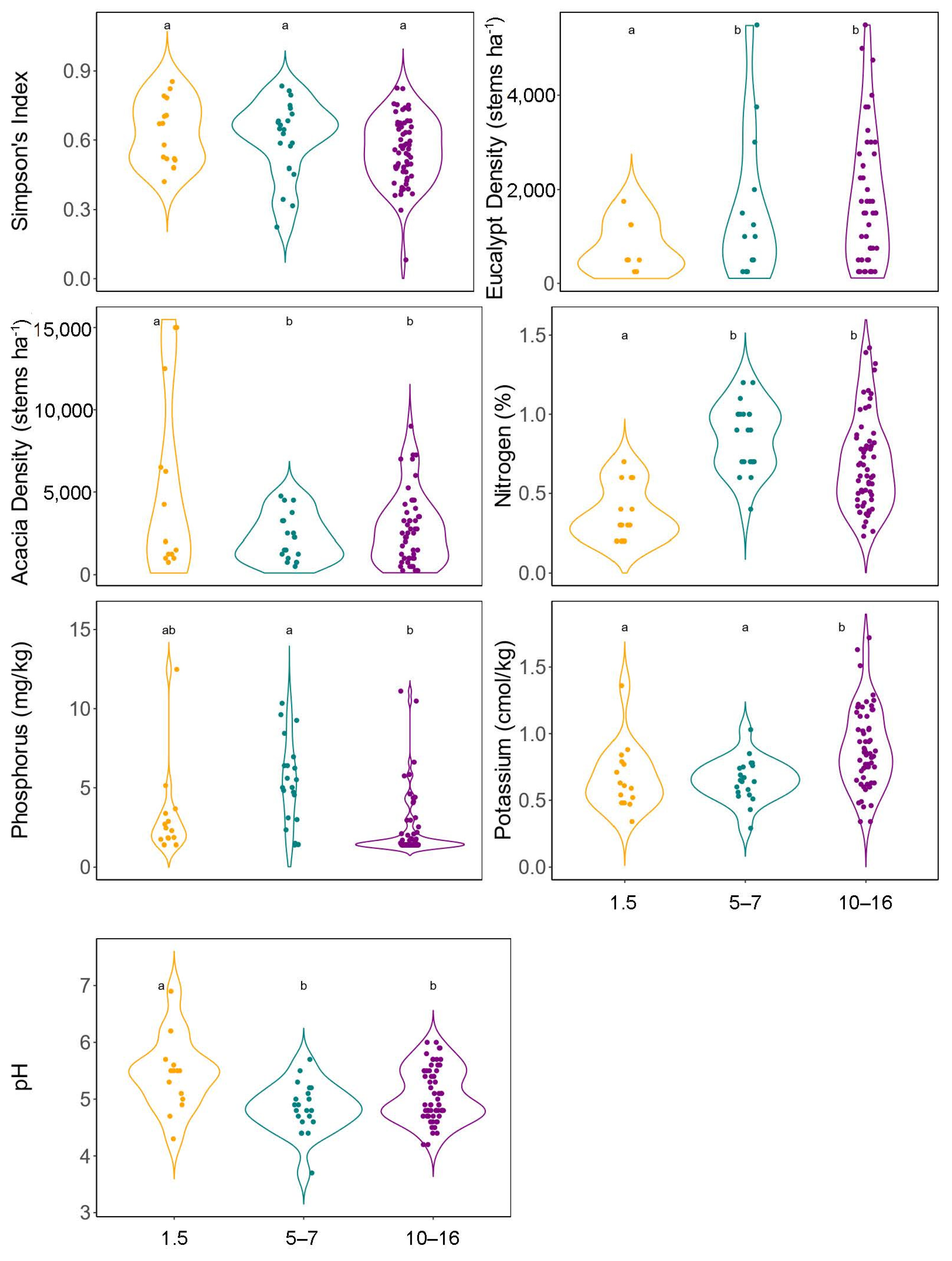
We assessed the effect of stand age on species diversity (Simpson’s index), vegetation structure (Eucalyptus and Acacia density), and soil nutrients on species richness using linear models. All linear models were checked to ensure key modelling assumptions such as normality of the errors and homogeneity of variance were met, and log transformations were applied when appropriate. The Tukey–Kramer test was used to assess pairwise differences between the means when the overall null hypothesis of no differences between any of the means was rejected. All analyses were performed using R [51].
We conducted a joint analysis of the species communities in three stages. First, we used the mvabund package [52] to test the statistical effects of environmental predictors on plant community composition (presence–absence). The environmental predictors used were selected by generating a correlation matrix and eliminating variables that were highly correlated (Pearson correlations > |0.6|; [53], see Table S3). The selected variables were Acacia density, Eucalyptus density, annual heat moisture index (AHMI), topographic wetness index (TWI), nitrogen, phosphorus, and potassium. These selected variables represented structural, climatic, and edaphic factors; hereafter referred to as “environmental predictors” unless otherwise specified. Stand structure was selected over stand age as it more fully captures disturbance history and constraints on resource availability than broad-scale classification of stand age [17].
In the second part of the analysis, we used the boral package [54] to quantify the relative importance of environmental gradients on individual species occurrence and community composition. Briefly, boral used a generalised linear latent variable modelling framework to quantify multivariate and correlated responses through the inclusion of a small number of latent variables. Generalised linear latent variable models (GLLVMs) can account for and quantify the covariation between species beyond that explained by measured environmental predictors, which can arise because of direct associations between species and sites. By jointly estimating latent variable values per site and species response to these latent variables, we can explicitly model the total covariation of the plant community (as well as on a per-species basis) in a component explained by the measured predictors versus a residual component explained by the latent variables. This can subsequently be used to infer the relative roles of environmental filtering and biotic processes (say) in driving community composition [55]. Hui [54], Niku et al. [56], Warton et al. [57], and Ovaskainen et al. [58] provide a useful general introduction to using GLLVMs for joint modelling of communities. We fitted binomial GLLVMs to presence–absence data of the plant species from our 96 plots, where a Bernoulli distribution was assumed for the binary responses. Since the effect of environmental predictors can only be estimated when we have sufficient observations, we removed rare species (defined as occurring in ≤10% of the plots). This reduced the number of species available for analysis in the GLLVMs from 108 to 40. Rare species are often difficult to model, as there is typically insufficient information in the dataset to quantify their species–environment relationships. As we were interested in studying the influence of overstorey density on understorey species composition, we excluded post-harvest regenerated overstorey species (Acacia and Eucalyptus spp.) from the analysis. We selected a 90% credible interval as a suitable balance between precision and confidence and the cost-prohibitive alternative of increasing sample size [59].
Furthermore, we built multiple univariate and multivariate models in combination to quantify the effect of environmental predictors on species occurrence and community composition. We developed multiple models with two latent variables (Figure S1) where the environmental predictors were linear and calculated the Widely Applicable Information Criterion (WAIC) for the fitted models to select the best combination of predictors explaining community composition [60]. We performed variance partitioning using boral to quantify the variance explained by the measured predictors versus the latent variable, which is used for developing multiple environmental predictors on each species as well as on community composition.

3. Results

A total of 108 plant species from 45 families were recorded across 96 plots (Table S2). Of these, 61 were trees and shrubs (phanerophytes), and 48 were herbs, ferns, grasses, and sedges (non-phanerophytes). The family Asteraceae had the most species (n = 21), followed by Poaceae (n = 8). In the 5–16-year-old stands, the most frequent understorey species were in the families Poaceae (n = 8) and Dennstaedtiaceae (n = 2). The species with the highest abundances were Tetrarrhena juncea and Pteridium esculentum. Phanerophytes were most represented by the families Myrtaceae (n = 5) and Fabaceae (n = 7). Eucalyptus regnans was present in 95% of the studied plots followed by Acacia dealbata in 92% of all plots.
There were no significant differences in Simpson’s index of diversity among stand age classes (p ≥ 0.61). Both Eucalyptus and Acacia density increased with age (Figure 2). Soil phosphorus in 5–7-year-old stands exceeded those in the oldest stands, while potassium concentrations in the 10–16-year-old stands exceeded those in the two younger age classes (Figure 2). Nitrogen concentrations in the two older age classes were greater than in the youngest (1.5 years) stand (Figure 2). Soil pH in the youngest stands (1.5 years) exceeded that in the two older age classes (Figure 2).

3.1. Plant Community Composition and Response to Environmental Predictors

Plant community composition was significantly correlated with six out of the seven environmental predictors examined (Table 1). AHMI was the strongest predictor followed by TWI. Phosphorus was the best of the soil nutrient predictors, followed by potassium. Plant community composition was significantly related to Acacia density but not to Eucalyptus density (Table 1). We found that the best model that included all environmental predictors had a WAIC of 3139, which was lower than the null model WAIC (3236). Details of all models that performed better than the null model are provided in Table S4.

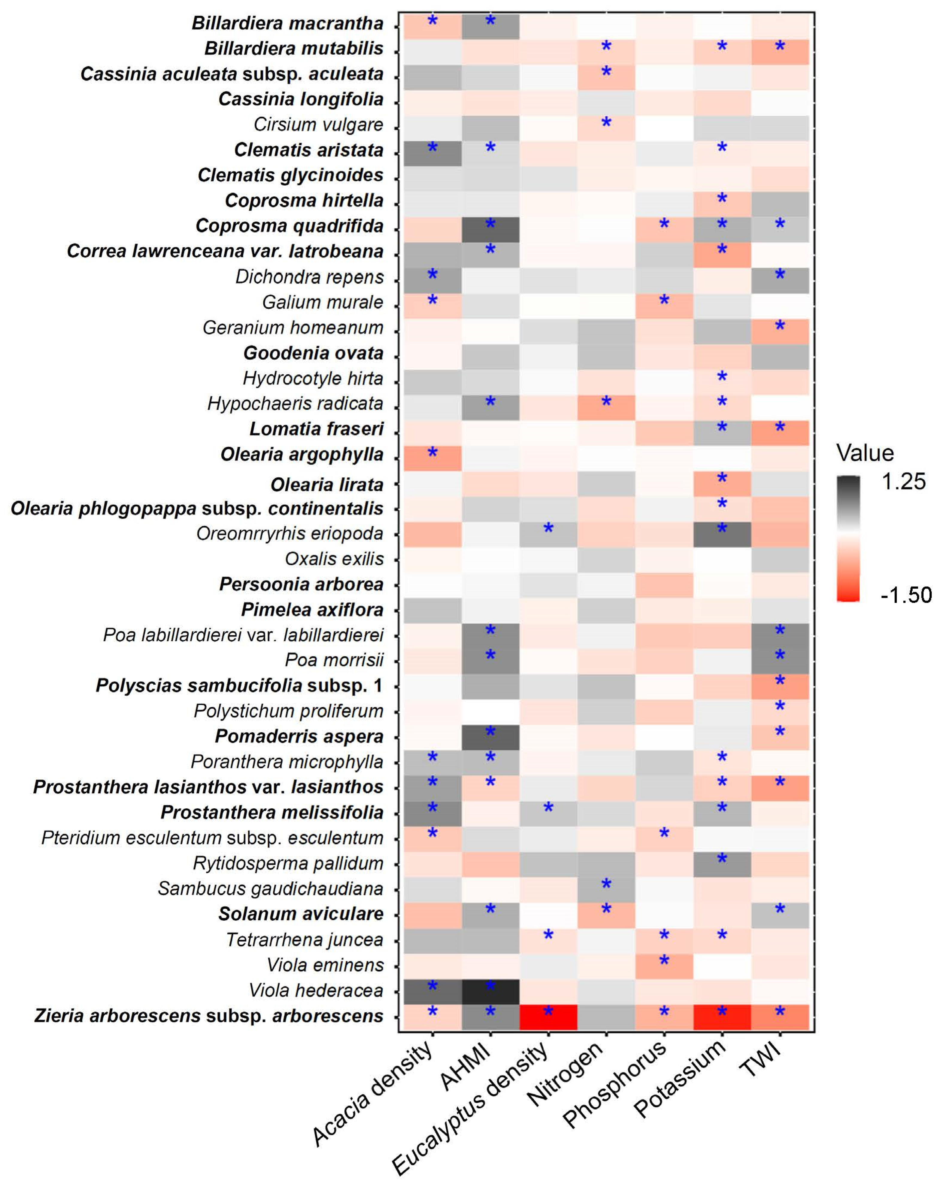
3.2. Species-Specific Responses to Environmental Predictors

Of the 40 species studied, 34 had statistically significant relationships with one or more of the model predictors. Of the seven predictors selected by WAIC for model inclusion, potassium had the strongest effect, followed by AHMI and TWI. Of the 17 species with significant responses to potassium, 13 also responded significantly to either AHMI or TWI (Figure 3). Six species responded positively, and five species responded negatively to an increase in Acacia density. Six species (Cassinia longifolia, Clematis glycinoides, Goodenia ovata, Oxalis exilis, Persoonia arborea, and Pimelea axiflora) were not associated with any of the predictors. Coprosma quadrifida and Prostanthera lasianthos var. lasianthos had relationships with four of the seven predictors. Zieria arborescens subsp. arborescens had a significant relationship with six of the seven predictors. Out of 40 species, 18 had either a positive or negative relationship with the moisture availability variables AHMI and TWI (Figure 3). A total of 13 species were significantly influenced by TWI, 8 negatively and 5 positively. Twelve species responded positively to AHMI and Prostanthera lasianthos var. lasianthos responded negatively with this species also negatively affected by TWI (Figure 3).
For the fitted GLLVM, environmental predictors explained more than 50% of the variance for 14 species with the latent variables accounting for the residual variance not explained by the measured environmental covariates (Figure 4). Across the 40 species, the environmental factors accounted for an average of 41% of the total covariation in the species community. On average, AHMI and TWI each explained 7% of the variance, overstorey explained 11%, and soil nutrients explained 14%. Overstorey explained 30% of the variance on average for the species, which had a significant response to the variable (Figure 4). The highest variance explained was for Billardiera macrantha (80%), with structure accounting for 31% of the variance. AHMI explained 29% of the variance for Coprosma quadrifida, Viola hederacea, and Pomaderris aspera. TWI explained 26% of the variance for Lomatia fraseri. Soil nutrients had the strongest influence on Viola eminens (41%) and Zieria arborescens subsp. arborescens (33%, Figure 4).

4. Discussion

Multiple factors shape the community composition of post-logging regrowth forests in temperate forests of southeastern Australia. Our findings highlight that during the earliest stages of the stand initiation phase of stand development, the plant community is systematically shaped by edaphic and climatic factors, and further filtered by stand structure and composition of the canopy species. Aridity, edaphic, topographic, and structural factors all contribute to shaping species occurrence and turnover. Aridity and topography filtered species across moisture gradients both within and across sites, while nutrients filtered species across gradients of N, P, and K availability. However, species occurrence and composition patterns associated with these gradients were also modified by Acacia density. The potential for Acacia in shaping plant composition in the region is the subject of increasing attention, particularly with respect to regeneration following forest harvesting [61] and the potential loss of obligate seeding forests and conversion to alternative states associated with increases in fire frequency due to climate change [62]. Bowd et al. [63], using an experimental manipulative approach, demonstrated a decline in understorey species richness resulting from Eucalyptus regeneration failure and increased dominance of Acacia in the overstorey. Furthermore, using remote sensing techniques, Singh et al. [61] demonstrated that increasing aggregation and number of patches of Acacia had a significant negative effect on plant beta diversity. The significant influence of Acacia has implications for comparing plant diversity between young stands that establish after logging or fire since logged areas typically have greater densities of Acacia than those subject to wildfire [29,30,31]. Increased abundance of Acacia in post-logging regrowth forests may act as a filter, encouraging the recruitment of some species and reducing the recruitment of other species within sites where abiotic factors (i.e., soil nutrition, climate, and soil moisture availability) are suitable for species to occur. This requires further work explicitly examining the interaction between Acacia density and environmental factors.

4.1. Canopy Structure and Density in Mediating Resource Availability

The lack of response to Eucalyptus density in our study suggests that the density of Eucalyptus may not have a significant impact on plant diversity during the earliest stages of stand development. This contrasts with the significant influence of Acacia density on plant community composition and turnover. Furthermore, using remote sensing imagery, Singh et al. [61] demonstrated that at the coupe scale, increasing aggregation of Acacia had a negative influence, and a number of patches of Eucalyptus had a positive influence on beta diversity in 10–16-year-old regrowth stands. In Australian eucalypt forests, light availability on the forest floor can reach high levels (~50%, [64]) compared to many other temperate closed canopy forests because of the vertical foliage and shallow leaf angles in Eucalyptus [65]. This contrasts with greater light interception under mixed to pure stands of Acacia, where light interception can reach 80% [66]. This finding has implications for future understanding of plant diversity and community composition in these forests, as more frequent fires are expected to cause a shift towards greater Acacia dominance in the region, e.g., [62]. Trouvé et al. [32] found that Eucalyptus regeneration in post-logging regrowth forests was less dense and more homogeneous than in post-fire regrowth. They suggested these differences could lead to different patterns in structural variability and consequences for stand development and associated understorey species composition [32].
Overstorey structure has been found to influence understorey plant species diversity in many ecosystems [67], including Australian temperate forests [33,68]. The wet sclerophyll forests of the Central Highlands are dominated by shade-intolerant Acacia and Eucalyptus species, which establish and grow rapidly (1–2 m in height per year) in the first decade post-disturbance [69]. In many stands, Acacia and Eucalyptus co-occur; however, as the stand matures, they often co-vary in abundance [70]. This is due to the difference in height of mature trees of each species (70–90 m for Eucalyptus vs. 20–25 m for Acacia) and the consequent overtopping and suppressive effect of the Eucalyptus. In this study, we examined forests in the earliest stages of stand development when the heights of Eucalyptus and Acacia are roughly equivalent and canopy stratification has not yet occurred. During this period, the canopy of the dense regrowth stands that develop reduces the amount of light reaching the forest floor while belowground competition for resources increases [71,72,73,74].

4.2. Species Responses

Species-specific responses were complex and variable. Our discussion focuses on species with the strongest model response, those common to this forest type, contrasting fire response strategies, and the response of threatened species.
Our model explained the greatest variance for Billardiera macrantha (80%), a climber that was negatively associated with Acacia density and positively related to AHMI. This species, however, only occupied 8% of sites, so in this case, the strong effect reflects just a slight decline in frequency with Acacia from a low base with similar low frequency reported by White and Vesk [75]. In contrast, Clematis aristata, another climber with a high proportion of explained variance (70%) was common to the study sites (46%) and responded positively to Acacia density. The difference in response in these two climbers may be explained by contrasting responses to logging disturbance [75], an association of B. macrantha with earlier successional stages and associated higher light environments, and for C. aristata as shade tolerant and common in early to mature successional stages in this forest type [33].
Tetrrahena juncea was the most common understorey species (85% of sites) across our study sites and is common to E. regnans forests, where it typically increases in abundance following disturbance [76,77]. The species was negatively associated with Eucalyptus density which explained the greatest proportion of variation, consistent with other work reporting an increase in abundance in T. juncea with a decline in canopy cover and associated increases in light availability and decline in soil moisture [76,78]. This positive association between reduction in canopy cover and increased dominance of T. juncea may increase forest flammability [76]. Combined with our earlier findings that regeneration failure of Eucalyptus was associated with drought at the landscape scale [61], this study lends further support to the potential for T. juncea to create positive, fire-flammability feedback in E. regnans forests under warmer and drier conditions associated with climate change [76], providing that moisture availability does not also become limiting to T. juncea [79].
The obligate seeder Zieria arborescens was negatively associated with Acacia and Eucalyptus density and occurred on drier sites lower in phosphorus and potassium. In contrast, Kasel et al. [33] and White and Vesk [75] found that the species occurred on microsites with higher moisture and shading, suggesting that Zieria arborescens is shade tolerant and likely not affected by overstorey composition. White and Vesk [75] noted that this species was typically absent in regrowth coupes and attributed this to seed death from high-intensity regeneration fires. In contrast, we found Zieria arborescens in 5–16-year-old harvested regrowth stands, consistent with Ough [29], who found the species was similarly frequent in 5–13-year-old clearfell sites and 10-year-old wildfire sites. The discrepancy in shade tolerance versus our negative association with overstorey density may be due to differences in edaphic and climatic conditions among the studies, as well as differences in stocking of Eucalyptus with poorly stocked coupes providing for higher densities of Acacia [30,61,63].
Pomaderris aspera is an obligate seeder that regenerates on a mass following fire from large soil seed banks [33,80]. Consistent with other studies [29,31,81], this species was the most frequently recorded understorey tree in our harvested regrowth stands. Like Zieria arborescens, Pomaderris aspera was located on drier sites but was not associated with an overstorey canopy. Pomaderris aspera was most common in the 10–16-year-old stands, where it competes with Acacia and Eucalyptus for resources until being overtopped and becoming suppressed; however, it can persist under low-light conditions for more than 50 years [73,82,83].
Resprouting species such as Olearia argophylla are often more abundant in wildfire regeneration than after clearfell [29,84] or salvage harvesting [31]. This is often explained by the increased sensitivity of resprouting organs to damage, desiccation, and death from mechanical disturbance, soil compaction, and displacement associated with harvesting [85,86]. We found Olearia argophylla across many of our plots in logged regrowth forests. However, like many other species, it was negatively affected by Acacia density. The higher density of Acacia in post-logging regrowth forests that Bowd et al. [31,63] observed may help explain the decline in Olearia argophylla they found in harvested sites relative to wildfire-impacted sites.
Persoonia arborea is a threatened species, endemic to the Central Highlands of Victoria and classified as critically endangered under the IUCN red list [87]. We found this species regenerates following disturbance associated with harvesting, which is consistent with other studies for this species [84,88] and additional species in this genus more broadly (e.g., P. hirsuta [89]). Although P. arborea was not significantly associated with any one variable, our model explained 34% of the variance in Persoonia arborea, with soil nutrition (14%) and canopy structure (10%) making the greatest contribution.
Together, these results suggest that patterns of species occurrence or turnover do not respond to the management of the forests in a simple manner but that environmental filtering plays a significant role in shaping community composition.

4.3. Effect of Soil Nutrients on Plant Community Composition

Australian soils are old and highly weathered, with low soil available phosphorus (P) [90,91]. Phosphorus availability had a strong influence on plant community composition in these regrowth stands. Kasel et al. [17] also found that available soil P, in combination with magnesium (Mg) and nitrogen (N), acted as edaphic filters in shaping the community composition across a range of fire histories in temperate forests across the Central Highlands. Nitrogen varied across different stand age classes, which may be due to an influx of nutrients in the early stages of stand development [92,93,94]. We found no relationship between soil nitrogen and the density of N-fixing Acacia. Our findings indicate that plant species composition is driven more by soil nutrients (especially N, P, and K) than stand structure, consistent with findings for the 1939 cohort of these forest types regenerating from wildfire [33]. This relationship raises important questions about how the variability in nutrients across time and scale explains species turnover and occurrence. This likely represents an ultimately limiting factor in combination with other variables, such as moisture, for filtering species composition.

4.4. Effect of Moisture Variables on the Plant Community Composition

AHMI and TWI were the environmental variables most strongly associated with plant community composition in post-logging regrowth in the Central Highlands. These factors represent moisture availability at two scales. Aridity (AHMI) has been found to be an important factor in shaping plant diversity [95]. More recently, Kasel et al. [17,33] found that climate was important in explaining the beta diversity of plant communities in the Central Highlands and more important for phanerophytes than non-phanerophytes. We found that TWI and AHMI (proxies for moisture availability) explained the most variance for phanerophytes. This suggests that non-phanerophytes are more affected by local microclimatic and edaphic conditions than phanerophytes, a finding that is supported by other studies, e.g., [13,17,33,96,97].

5. Conclusions

While many studies on plant community composition in the young forests developing after timber harvesting have discussed the role of biological legacies and their influence on plant diversity, few have considered the influence of environmental factors that may be filtering plant community composition. Our study demonstrated the initial community compositions were shaped by soil nutrient and moisture availability at fine scales and climatic conditions at broad scales. In addition, variability in the density of Acacia in these young stands further influences community composition by favouring some species and disadvantaging others, leading to complex patterns across scales in plant community composition. Forest dynamics are complex, and our study highlights how different factors affect the development of the vegetation communities for stand development in post-logging regrowth forests. Future studies which explore interactions among biotic and abiotic factors and how regeneration patterns diverge between forests affected by logging or by fire should account for these factors. This will provide more rigorous insights into how stand development after timber harvesting may [30,31] or may not [35] diverge from stand development patterns. From a management perspective, interventions such as thinning could be used to promote plant species diversity in areas supporting dense patches of Acacia in the early stages of stand development. However, any manipulation of Acacia density must also consider the importance of this species as a habitat for the critically endangered Leadbeater’s Possum [70,98].

Supplementary Materials

The following supporting information can be downloaded at: https://www.mdpi.com/article/10.3390/f14061166/s1, Figure S1: Model-based unconstrained and residual ordination biplot for the plant. Each of the 96 sites is labelled by number starting from 1 to 96. Dark green colour represents 1.5 years, brown colour represents 5–7-year-old, and black represents 10–16-year-old plot; Table S1: Coupe number, coupe age class (time since harvesting), and associated environmental variables. There were three plots within each coupe; Table S2: Summary of family and species recorded across all plots. Life form: phanerophytes (woody) and non-phanerophytes (non-woody) and frequency are provided. There were 96 plots across three different age classes, and total number of species present was 108. Species are ordered by Family; Table S3: Mean and standard deviation of the covariate predictors within each age group. Those not correlated (r < |0.6|) with other covariates (and used in model predictions) are indicated in bold. SD, standard deviation; Table S4: Widely applicable Information Criterion (WAIC) for various binomial GLLVMs fitted using boral.

Author Contributions

Conceptualization, A.S., C.R.N., P.J.B. and S.K.; methodology, all authors; formal analysis, A.S., F.K.C.H. and R.T.; investigation, A.S.; resources, C.R.N., P.J.B. and S.K.; data curation, A.S.; writing—original draft preparation, A.S.; writing—review and editing, all authors; visualization, A.S.; supervision, C.R.N., P.J.B. and S.K.; project administration, C.R.N.; funding acquisition, A.S., C.R.N., P.J.B. and S.K. All authors have read and agreed to the published version of the manuscript.

Funding

This research was funded by the Australian Research Council (LP140100580 to CN and PJB, FT120100715 to P.J.B.). A.S. was supported by the University of Melbourne through a Melbourne Research Scholarship. C.N. and S.K. were additionally funded through the Integrated Forest Ecosystem Research (IFER) program of the Victoria government Department of Energy, Environment and Climate Action, agreement number 301103. Additional funding was generously provided to A.S., S.K. and C.N. by Eucalypt Australia.

Data Availability Statement

Please contact the corresponding author regarding the availability of underlying data.

Acknowledgments

We would like to thank Benjamin Smith, Benjamin Wagner, Carola Pritzkow, Linda Parker, Zheng Zhang, Thiet Van Nguyen, and Kaitlyn Hammond for their help with the fieldwork.

Conflicts of Interest

The authors declare no conflict of interest. The funders had no role in the design of this study; in the collection, analyses, or interpretation of data; in the writing of the manuscript; or in the decision to publish the results.

References

  1. Chase, J.M.; Myers, J.A. Disentangling the importance of ecological niches from stochastic processes across scales. Philos. Trans. R. Soc. Lond. B Biol. Sci. 2011, 366, 2351–2363. [Google Scholar] [CrossRef] [PubMed] [Green Version]
  2. Hutchinson, G.E. Concluding remarks in Populations studies: Animal Ecology and Demography. In Cold Spring Harbor Symposia on Quantitative Biology; Cold Spring Harbor: New York, NY, USA, 1957; pp. 415–427. [Google Scholar]
  3. Austin, M.P. A silent clash of paradigms: Some inconsistencies in community ecology. Oikos 1999, 86, 170–178. [Google Scholar] [CrossRef]
  4. Eilts, J.A.; Mittelbach, G.G.; Reynolds, H.L.; Gross, K.L. Resource heterogeneity, soil fertility, and species diversity: Effects of clonal species on plant communities. Am. Nat. 2011, 177, 574–588. [Google Scholar] [CrossRef] [PubMed]
  5. Forrester, D.I. The spatial and temporal dynamics of species interactions in mixed-species forests: From pattern to process. For. Ecol. Manag. 2014, 312, 282–292. [Google Scholar] [CrossRef]
  6. Gosper, C.R.; Yates, C.J.; Prober, S.M. Floristic diversity in fire-sensitive eucalypt woodlands shows a “U”-shaped relationship with time since fire. J. Appl. Ecol. 2013, 50, 1187–1196. [Google Scholar] [CrossRef]
  7. Bruno, J.F.; Stachowicz, J.J.; Bertness, M.D. Inclusion of facilitation into ecological theory. Trends Ecol. Evol. 2003, 18, 119–125. [Google Scholar] [CrossRef]
  8. Kumar, P.; Chen, H.Y.; Thomas, S.C.; Shahi, C. Linking resource availability and heterogeneity to understorey species diversity through succession in boreal forest of Canada. J. Ecol. 2018, 106, 1266–1276. [Google Scholar] [CrossRef]
  9. Su, X.; Wang, M.; Huang, Z.; Fu, S.; Chen, H.Y. Forest understorey vegetation: Colonization and the Availability and Heterogeneity of resources. Forests 2019, 10, 944. [Google Scholar] [CrossRef] [Green Version]
  10. Reich, P.B.; Frelich, L.E.; Voldseth, R.A.; Bakken, P.; Adair, E.C. Understorey diversity in southern boreal forests is regulated by productivity and its indirect impacts on resource availability and heterogeneity. J. Ecol. 2012, 100, 539–545. [Google Scholar] [CrossRef]
  11. Veldman, J.W.; Brudvig, L.A.; Damschen, E.I.; Orrock, J.L.; Mattingly, W.B.; Walker, J.L. Fire frequency, agricultural history and the multivariate control of pine savanna understorey plant diversity. J. Veg. Sci. 2014, 25, 1438–1449. [Google Scholar] [CrossRef]
  12. Siefert, A.; Ravenscroft, C.; Althoff, D.; Alvarez-Yépiz, J.C.; Carter, B.E.; Glennon, K.L.; Heberling, J.M.; Jo, I.S.; Pontes, A.; Sauer, A.; et al. Scale dependence of vegetation-environment relationships: A meta-analysis of multivariate data. J. Veg. Sci. 2012, 23, 942–951. [Google Scholar] [CrossRef]
  13. Chick, M.P.; Nitschke, C.R.; Cohn, J.S.; Penman, T.D.; York, A. Factors influencing above-ground and soil seed bank vegetation diversity at different scales in a quasi-Mediterranean ecosystem. J. Veg. Sci. 2018, 29, 684–694. [Google Scholar] [CrossRef]
  14. Bartels, S.F.; Chen, H.Y. Is understory plant species diversity driven by resource quantity or resource heterogeneity? Ecology 2010, 91, 1931–1938. [Google Scholar] [CrossRef] [PubMed]
  15. Paudel, S.K.; Waeber, P.O.; Simard, S.W.; Innes, J.L.; Nitschke, C.R. Multiple factors influence plant richness and diversity in the cold and dry boreal forest of southwest Yukon, Canada. Plant. Ecol. 2016, 217, 505–519. [Google Scholar] [CrossRef]
  16. Barbier, S.; Gosselin, F.; Balandier, P. Influence of tree species on understory vegetation diversity and mechanisms involved—A critical review for temperate and boreal forests. For. Ecol. Manag. 2008, 254, 1–15. [Google Scholar] [CrossRef]
  17. Kasel, S.; Bennett, L.T.; Aponte, C.; Fedrigo, M.; Nitschke, C.R. Environmental heterogeneity promotes floristic turnover in temperate forests of south-eastern Australia more than dispersal limitation and disturbance. Landsc. Ecol. 2017, 32, 1613–1629. [Google Scholar] [CrossRef]
  18. Harvey, B.J.; Holzman, B.A. Divergent successional pathways of stand development following fire in a California closed-cone pine forest. J. Veg. Sci. 2014, 25, 88–99. [Google Scholar] [CrossRef]
  19. Connell, J.H.; Slatyer, R.O. Mechanisms of succession in natural communities and their role in community stability and organization. Am. Nat. 1977, 111, 1119–1144. [Google Scholar] [CrossRef]
  20. Clements, F.E. Plant Succession: An Analysis of the Development of Vegetation; Carnegie Institution of Washington: Washington, DC, USA, 1916. [Google Scholar]
  21. Egler, F.E. Vegetation science concepts I. Initial floristic composition, a factor in old-field vegetation development with 2 figs. Plant. Ecol. 1954, 4, 412–417. [Google Scholar] [CrossRef]
  22. Cole, D.; Rapp, M. Elemental cycling in forest ecosystems. In Dynamic Properties of Forest Ecosystems; Reichle, D.E., Ed.; International Biological Programme; Cambridge University Press: Cambridge, UK, 1981; pp. 341–409. [Google Scholar]
  23. Wilson, S.D.; Tilman, D. Plant competition and resource availability in response to disturbance and fertilization. Ecology 1993, 74, 599–611. [Google Scholar] [CrossRef]
  24. Forrester, D.I.; Bauhus, J. A Review of Processes Behind Diversity-Productivity Relationships in Forests. Curr. Rep. 2016, 2, 45–61. [Google Scholar] [CrossRef] [Green Version]
  25. Richards, A.E.; Forrester, D.I.; Bauhus, J.; Scherer-Lorenzen, M. The influence of mixed tree plantations on the nutrition of individual species: A review. Tree Physiol. 2010, 30, 1192–1208. [Google Scholar] [CrossRef] [Green Version]
  26. Bartels, S.F.; Chen, H.Y. Interactions between overstorey and understorey vegetation along an overstorey compositional gradient. J. Veg. Sci. 2013, 24, 543–552. [Google Scholar] [CrossRef]
  27. Bartemucci, P.; Messier, C.; Canham, C.D. Overstory influences on light attenuation patterns and understory plant community diversity and composition in southern boreal forests of Quebec. Can. J. For. Res. 2006, 36, 2065–2079. [Google Scholar] [CrossRef] [Green Version]
  28. Bratton, S.P. Resource division in an understory herb community: Responses to temporal and microtopographic gradients. Am. Nat. 1976, 110, 679–693. [Google Scholar] [CrossRef]
  29. Ough, K. Regeneration of Wet Forest flora a decade after clear-felling or wildfire-is there a difference? Aust. J. Bot. 2001, 49, 645–664. [Google Scholar] [CrossRef]
  30. Blair, D.P.; McBurney, L.M.; Blanchard, W.; Banks, S.C.; Lindenmayer, D.B. Disturbance gradient shows logging affects plant functional groups more than fire. Ecol. Appl. 2016, 26, 2280–2301. [Google Scholar] [CrossRef] [Green Version]
  31. Bowd, E.J.; Lindenmayer, D.B.; Banks, S.C.; Blair, D.P. Logging and fire regimes alter plant communities. Ecol. Appl. 2018, 28, 826–841. [Google Scholar] [CrossRef] [Green Version]
  32. Trouvé, R.; Sherriff, R.M.; Holt, L.M.; Baker, P.J. Differing regeneration patterns after catastrophic fire and clearfelling: Implications for future stand dynamics and forest management. For. Ecol. Manag. 2021, 498, 119555. [Google Scholar] [CrossRef]
  33. Kasel, S.; Nitschke, C.R.; Baker, S.C.; Pryde, E.C. Concurrent assessment of functional types in extant vegetation and soil seed banks informs environmental constraints and mechanisms of plant community turnover in temperate forests of south-eastern Australia. For. Ecol. Manag. 2022, 519, 14. [Google Scholar] [CrossRef]
  34. Pulsford, S.A.; Lindenmayer, D.B.; Driscoll, D.A. A succession of theories: Purging redundancy from disturbance theory. Biol. Rev. 2016, 91, 148–167. [Google Scholar] [CrossRef]
  35. Attiwill, P.M. Ecological disturbance and the conservative management of eucalypt forests in Australia. For. Ecol. Manag. 1994, 63, 301–346. [Google Scholar] [CrossRef]
  36. ABARES. Australia’s State of the Forest Report 2018; ABARES: Canberra, ACT, Australia, 2018. [Google Scholar]
  37. Stewart, S.B.; Nitschke, C.R. Improving temperature interpolation using MODIS LST and local topography: A comparison of methods in south east Australia. Int. J. Climatol. 2017, 37, 3098–3110. [Google Scholar] [CrossRef]
  38. Keenan, R.J.; Nitschke, C. Forest management options for adaptation to climate change: A case study of tall, wet eucalypt forests in Victoria’s Central Highlands region. Aust. For. 2016, 79, 96–107. [Google Scholar] [CrossRef]
  39. Booth, T.H.; Pryor, L.D. Climatic requirements of some commercially important eucalypt species. For. Ecol. Manag. 1991, 43, 47–60. [Google Scholar] [CrossRef]
  40. Adams, M.A.; Attiwill, P.M. Nutrient cycling and nitrogen mineralization in eucalypt forests of south-eastern Australia. Plant. Soil. 1986, 92, 341–362. [Google Scholar] [CrossRef]
  41. Ashton, D.H. Studies on the Autecology of Eucalyptus regnans F.v. M. Ph.D. Thesis, The University of Melbourne, Melbourne, VIC, Australia, 1956. [Google Scholar]
  42. Squire, R.; Geary, P.; Lutze, M. The East Gippsland Silvicultural Systems Project. I: The establishment of the project in lowland forest. Aust. For. 2006, 69, 167–181. [Google Scholar] [CrossRef]
  43. Dignan, P. Wood Production in Mountain Ash Forests: Implications of Alternative Systems for Harvesting Operations; VSP Technical Report. No. 22; Department of Conservation and Natural Resources: East Melbourne, VIC, Australia, 1993. [Google Scholar]
  44. Squire, R.O.; Campbell, R.G.; Wareing, K.J.; Featherston, G.R. The mountain ash forests of Victoria: Ecology, silviculture and management for wood production. In Forest Management in Australia, Proceedings of the Conference of the Institute of Foresters of Australia, Perth, WA, Australia, 18–22 September 1987; McKinnell, F.H., Hopkins, E.R., Fox, J.E.P., Eds.; Surrey Beatty & Sons: Chipping Norton, NSW, Australia, 1991; pp. 36–57. [Google Scholar]
  45. Keenan, R.J.; Kimmins, J.P. The ecological effects of clear-cutting. Environ. Rev. 1993, 1, 121–144. [Google Scholar] [CrossRef]
  46. Fedrigo, M.; Stewart, S.B.; Roxburgh, S.H.; Kasel, S.; Bennett, L.T.; Vickers, H.; Nitschke, C.R. Predictive Ecosystem Mapping of South-Eastern Australian Temperate Forests Using Lidar-Derived Structural Profiles and Species Distribution Models. Remote. Sens. 2019, 11, 93. [Google Scholar] [CrossRef] [Green Version]
  47. Wang, T.; Hamann, A.; Yanchuk, A.; O’neill, G.; Aitken, S.N. Use of response functions in selecting lodgepole pine populations for future climates. Glob. Change Biol. 2006, 12, 2404–2416. [Google Scholar] [CrossRef]
  48. Raduła, M.W.; Szymura, T.H.; Szymura, M. Topographic wetness index explains soil moisture better than bioindication with Ellenberg’s indicator values. Ecol. Indic. 2018, 85, 172–179. [Google Scholar] [CrossRef]
  49. Rayment, G.E.; Lyons, D.J. Soil Chemical Methods: Australasia; CSIRO Publishing: Collingwood, VIC, Australia, 2010. [Google Scholar]
  50. Rayment, G.E.; Higginson, F.R. Australian Laboratory Handbook of Soil and Water Chemical Methods; Inkata Press: Port Melbourne, VIC, Australia, 1992. [Google Scholar]
  51. R Core Team. R: A Language and Environment for Statistical Computing; R Foundation for Statistical Computing: Vienna, Austria, 2019. [Google Scholar]
  52. Wang, Y.; Naumann, U.; Wright, S.T.; Warton, D.I. mvabund—An R package for model-based analysis of multivariate abundance data. Methods Ecol. Evol. 2012, 3, 471–474. [Google Scholar] [CrossRef]
  53. Dormann, C.F.; Elith, J.; Bacher, S.; Buchmann, C.; Carl, G.; Carré, G.; Marquéz, J.R.G.; Gruber, B.; Lafourcade, B.; Leitão, P.J.; et al. Collinearity: A review of methods to deal with it and a simulation study evaluating their performance. Ecography 2013, 36, 27–46. [Google Scholar] [CrossRef]
  54. Hui, F.K.C. boral—Bayesian Ordination and Regression Analysis of Multivariate Abundance Data in r. Methods Ecol. Evol. 2016, 7, 744–750. [Google Scholar] [CrossRef] [Green Version]
  55. Björk, J.R.; Hui, F.K.C.; O’Hara, R.B.; Montoya, J.M. Uncovering the drivers of host-associated microbiota with joint species distribution modelling. Mol. Ecol. 2018, 27, 2714–2724. [Google Scholar] [CrossRef] [PubMed]
  56. Niku, J.; Hui, F.K.C.; Taskinen, S.; Warton, D.I.; Goslee, S. gllvm: Fast analysis of multivariate abundance data with generalized linear latent variable models in R. Methods Ecol. Evol. 2019, 10, 2173–2182. [Google Scholar] [CrossRef] [Green Version]
  57. Warton, D.I.; Blanchet, F.G.; O’Hara, R.B.; Ovaskainen, O.; Taskinen, S.; Walker, S.C.; Hui, F.K.C. So Many Variables: Joint Modeling in Community Ecology. Trends Ecol. Evol. 2015, 30, 766–779. [Google Scholar] [CrossRef] [PubMed]
  58. Ovaskainen, O.; Tikhonov, G.; Norberg, A.; Guillaume Blanchet, F.; Duan, L.; Dunson, D.; Roslin, T.; Abrego, N. How to make more out of community data? A conceptual framework and its implementation as models and software. Ecol. Lett. 2017, 20, 561–576. [Google Scholar] [CrossRef] [Green Version]
  59. Di Stefano, J. How Much Power Is Enough? Against the Development of an Arbitrary Convention for Statistical Power Calculations. Funct. Ecol. 2003, 17, 707–709. [Google Scholar] [CrossRef]
  60. Watanabe, S.; Opper, M. Asymptotic equivalence of Bayes cross validation and widely applicable information criterion in singular learning theory. J. Mach. Learn. Res. 2010, 11, 3571–3594. [Google Scholar]
  61. Singh, A.; Wagner, B.; Kasel, S.; Baker, P.J.; Nitschke, C.R. Canopy Composition and Spatial Configuration Influences Beta Diversity in Temperate Regrowth Forests of Southeastern Australia. Drones 2023, 7, 155. [Google Scholar] [CrossRef]
  62. Fairman, T.A.; Nitschke, C.R.; Bennett, L.T. Too much, too soon? A review of the effects of increasing wildfire frequency on tree mortality and regeneration in temperate eucalypt forests. Int. J. Wildland Fire 2016, 25, 831–848. [Google Scholar] [CrossRef]
  63. Bowd, E.J.; McBurney, L.; Lindenmayer, D.B. The characteristics of regeneration failure and their potential to shift wet temperate forests into alternate stable states. For. Ecol. Manag. 2023, 529, 120673. [Google Scholar] [CrossRef]
  64. Anderson, M.C. The geometry of leaf distribution in some south-eastern Australian forests. Agric. Meteorol. 1981, 25, 195–206. [Google Scholar] [CrossRef]
  65. King, D.A. The functional significance of leaf angle in Eucalyptus. Aust. J. Bot. 1997, 45, 619–639. [Google Scholar] [CrossRef]
  66. Bauhus, J.; Van Winden, A.P.; Nicotra, A.B. Aboveground interactions and productivity in mixed-species plantations of Acacia mearnsii and Eucalyptus globulus. Can. J. For. Res. 2004, 34, 686–694. [Google Scholar] [CrossRef]
  67. Thomas, S.C.; Halpern, C.B.; Falk, D.A.; Liguori, D.A.; Austin, K.A. Plant diversity in managed forests: Understory responses to thinning and fertilization. Ecol. Appl. 1999, 9, 864–879. [Google Scholar] [CrossRef]
  68. Baker, S.C.; Kasel, S.; van Galen, L.G.; Jordan, G.J.; Nitschke, C.R.; Pryde, E.C. Identifying regrowth forests with advanced mature forest values. For. Ecol. Manag. 2019, 433, 73–84. [Google Scholar] [CrossRef]
  69. May, B. Silver Wattle (Acacia dealbata): Its Role in the Ecology of the Mountain Ash Forest and the Effect of Alternative Silvicultural Systems on Its Regeneration. Ph.D. Thesis, The University of Melbourne, Melbourne, VIC, Australia, 1999. [Google Scholar]
  70. Trouvé, R.; Nitschke, C.R.; Andrieux, L.; Willersdorf, T.; Robinson, A.P.; Baker, P.J. Competition drives the decline of a dominant midstorey tree species. Habitat implications for an endangered marsupial. For. Ecol. Manag. 2019, 447, 26–34. [Google Scholar] [CrossRef]
  71. Ashton, D.H. The root and shoot development of Eucalyptus regnans F. Muell. Aust. J. Bot. 1975, 23, 867–887. [Google Scholar] [CrossRef]
  72. Ashton, D.H. The development of even-aged stands of Eucalyptus regnans F. Muell. in central Victoria. Aust. J. Bot. 1976, 24, 397–414. [Google Scholar] [CrossRef]
  73. Ashton, D.H. The big ash forest, Wallaby Creek, Victoria—Changes during one lifetime. Aust. J. Bot. 2000, 48, 1–26. [Google Scholar] [CrossRef]
  74. Forrester, D.I. Growth responses to thinning, pruning and fertiliser application in Eucalyptus plantations: A review of their production ecology and interactions. For. Ecol. Manag. 2013, 310, 336–347. [Google Scholar] [CrossRef]
  75. White, D.J.; Vesk, P.A. Fire and legacy effects of logging on understorey assemblages in wet-sclerophyll forests. Aust. J. Bot. 2019, 67, 341–357. [Google Scholar] [CrossRef]
  76. Cadiz, G.O.; Cawson, J.G.; Penman, T.D.; York, A.; Duff, T.J. Environmental factors associated with the abundance of forest wiregrass (Tetrarrhena juncea), a flammable understorey grass in productive forests. Aust. J. Bot. 2000, 68, 37–48. [Google Scholar] [CrossRef]
  77. Penman, T.D.; Binns, D.L.; Shiels, R.J.; Allen, R.M.; Kavanagh, R.P. Changes in understorey plant species richness following logging and prescribed burning in shrubby dry sclerophyll forests of south-eastern Australia. Austral Ecol. 2008, 33, 197–210. [Google Scholar] [CrossRef]
  78. Ashwell, D. The Importance of Tetrarrhena juncea in the Ecology of Eucalyptus regnans Stands. Master’s Thesis, The University of Melbourne, Parkville, VIC, Australia, 1985. [Google Scholar]
  79. Cadiz, G.O.; Cawson, J.G.; Duff, T.J.; Penman, T.D.; York, A.; Farrell, C. Independent effects of drought and shade on growth, biomass allocation and leaf morphology of a flammable perennial grass Tetrarrhena juncea R.Br. Plant. Ecol. 2021, 222, 877–895. [Google Scholar] [CrossRef]
  80. Younis, S.; Kasel, S. Do Fire Cues Enhance Germination of Soil Seed Stores across an Ecotone of Wet Eucalypt Forest to Cool Temperate Rainforest in the Central Highlands of South-Eastern Australia? Fire 2023, 6, 138. [Google Scholar] [CrossRef]
  81. Wang, L. The soil seed bank and understorey regeneration in Eucalyptus regnans forest, Victoria. Aust. J. Ecol. 1997, 22, 404–411. [Google Scholar] [CrossRef]
  82. Ashton, D. The seasonal growth of Eucalyptus regnans F. Muell. Aust. J. Bot. 1975, 23, 239–252. [Google Scholar] [CrossRef]
  83. Vickers, H.; Kasel, S.; Duff, T.; Nitschke, C. Recruitment and growth dynamics of a temperate forest understorey species following wildfire in southeast Australia. Dendrochronologia 2021, 67, 125829. [Google Scholar] [CrossRef]
  84. Murphy, A.; Ough, K. Regenerative strategies of understorey flora following clearfell logging in the Central Highlands, Victoria. Aust. For. 1997, 60, 90–98. [Google Scholar] [CrossRef]
  85. Ough, K.; Murphy, A. Decline in tree fern abundance after clearfell harvesting. For. Ecol. Manag. 2004, 199, 153–163. [Google Scholar] [CrossRef]
  86. Rab, M.A. Soil physical and hydrological properties following logging and slash burning in the Eucalyptus regnans forest of southeastern Australia. For. Ecol. Manag. 1996, 84, 159–176. [Google Scholar] [CrossRef]
  87. Weston, P.; Cameron, D. Persoonia arborea . In The IUCN Red List of Threatened Species 2020; IUCN: Gland, Switzerland, 2020; pp. 1–8. [Google Scholar]
  88. Gullan, P. A Rare Plant That Is Locally Abundant. Available online: http://www.viridans.com/RAREPL/locallyabundant.htm (accessed on 2 April 2023).
  89. Emery, N.J.; Offord, C.A. Managing Persoonia (Proteaceae) species in the landscape through a better understanding of their seed biology and ecology. Cunninghamia J. Plant. Ecol. East Aust. 2018, 18, 89–107. [Google Scholar]
  90. Adams, M.; Attiwill, P.; Polglase, P. Availability of nitrogen and phosphorus in forest soils in northeastern Tasmania. Biol. Fertil. Soils 1989, 8, 212–218. [Google Scholar] [CrossRef]
  91. Beadle, N. Soil phosphate and the delimitation of plant communities in eastern Australia. Ecology 1954, 35, 370–375. [Google Scholar] [CrossRef]
  92. Smithwick, E.A.H.; Turner, M.G.; Mack, M.C.; Chapin, F.S. Postfire Soil N Cycling in Northern Conifer Forests Affected by Severe, Stand-Replacing Wildfires. Ecosystems 2005, 8, 163–181. [Google Scholar] [CrossRef]
  93. Wan, S.; Hui, D.; Luo, Y. Fire effects on nitrogen pools and dynamics in terrestrial ecosystems: A meta-analysis. Ecol. Appl. 2001, 11, 1349–1365. [Google Scholar] [CrossRef]
  94. Weston, C.J.; Attiwill, P.M. Effects of fire and harvesting on nitrogen transformations and ionic mobility in soils of Eucalyptus regnans forests of south-eastern Australia. Oecologia 1990, 83, 20–26. [Google Scholar] [CrossRef]
  95. Kreft, H.; Jetz, W. Global patterns and determinants of vascular plant diversity. Proc. Natl. Acad. Sci. USA 2007, 104, 5925–5930. [Google Scholar] [CrossRef] [PubMed] [Green Version]
  96. Murphy, S.J.; Audino, L.D.; Whitacre, J.; Eck, J.L.; Wenzel, J.W.; Queenborough, S.A.; Comita, L.S. Species associations structured by environment and land-use history promote beta-diversity in a temperate forest. Ecology 2015, 96, 705–715. [Google Scholar] [CrossRef] [PubMed] [Green Version]
  97. Plue, J.; De Frenne, P.; Acharya, K.; Brunet, J.; Chabrerie, O.; Decocq, G.; Diekmann, M.; Graae, B.J.; Heinken, T.; Hermy, M.; et al. Where does the community start, and where does it end? Including the seed bank to reassess forest herb layer responses to the environment. J. Veg. Sci. 2017, 28, 424–435. [Google Scholar] [CrossRef]
  98. Baker, P.J.; Nitschke, C.R.; Trouve, R.; Robinson, A.P. Forest stand dynamics drive a conservation conundrum for the critically endangered Leadbeater’s Possum. In Forests as Complex Social and Ecological Systems: A Festschrift for Chadwick D. Oliver; Baker, P.J., Larsen, D.R., Saxena, A., Eds.; Springer International Publishing: Cham, Switzerland, 2022; pp. 93–113. [Google Scholar]
Figure 1. The Central Highlands of Victoria in southeastern Australia. Points represent the three different forest age classes surveyed (blue, 1.5 years; green, 5–7 years; black, 10–16 years).
Forests 14 01166 g001
Figure 2. Violin plots and pairwise Tukey–Kramer test for Simpson’s diversity, structure, soil nutrients, and pH across the three different stand age classes. Different letters above each boxplot bar indicate significant differences (p < 0.05) between age classes.
Forests 14 01166 g002
Figure 3. Species-specific regression coefficients for the seven environmental predictors included in the estimated binomial GLLVM from boral. Effects that were deemed to be significant are indicated by an ‘*’, where significance is based on whether species corresponded to 90% credible intervals excluding zero. Phanerophytes are indicated in bold, and non-phanerophytes in plain text.
Forests 14 01166 g003
Figure 4. Variance partitioning from the binomial GLLVM from boral. The entire bar represents the total variation explained by all the predictors for each species. AHMI, annual heat moisture index; TWI, topographic wetness index; Density, Eucalyptus and Acacia stem density; Soil nutrients, N, P, and K. Phanerophytes are indicated in bold, and non-phanerophytes in plain text. The latent variables explain the residual variance not accounted for by the measured environmental covariates.
Forests 14 01166 g004
Table 1. Summary of multivariate analysis (using mvabund) for testing the effects of environmental predictors on plant community composition. Predictors are ordered from highest to lowest.
Environmental PredictorsWald Statisticp Value
Annual heat moisture index231.910.001
Topographic wetness index121.440.001
Phosphorus104.280.001
Acacia density96.280.001
Potassium78.710.008
Nitrogen72.020.014
Eucalyptus density56.960.230
Disclaimer/Publisher’s Note: The statements, opinions and data contained in all publications are solely those of the individual author(s) and contributor(s) and not of MDPI and/or the editor(s). MDPI and/or the editor(s) disclaim responsibility for any injury to people or property resulting from any ideas, methods, instructions or products referred to in the content.

