Article

A Geoprocessing Tool for the Calculation of Primary Wood Transportation Distance

1
Department of Forest Management, National Forest Centre—Forest Research Institute Zvolen, T.G. Masaryka 22, 96001 Zvolen, Slovakia
2
Department of Forest Ecology, National Forest Centre—Forest Research Institute Zvolen, T.G. Masaryka 22, 96001 Zvolen, Slovakia
*
Author to whom correspondence should be addressed.
Forests 2023, 14(5), 907; https://doi.org/10.3390/f14050907
Submission received: 10 March 2023 / Revised: 24 April 2023 / Accepted: 26 April 2023 / Published: 27 April 2023
(This article belongs to the Special Issue Recent Advances in Forests Roads Research)

Abstract

:
Knowledge about wood transportation distances is essential for sustainable forest management and related decision making in forest protection against fire or flood events. In this context, we developed the geoprocessing tool TraDis to allow for the calculation of two-dimensional (2D) and three-dimensional (3D) distance between a forest stand and the nearest forest road (i.e., pre-skidding distance) and the distance between this road and the nearest hauling place (i.e., skidding distance). The first aim of this study is to present the workflow for the calculation of the primary wood transportation distance using the TraDis tool. A detailed description, flowchart, and scheme are provided for these purposes. The second aim is to present the applicability of this workflow through a case study. The study area included 391 ha of forest stands, 58 km of forest roads, and 18 hauling places, and the transportation distances were calculated for various target objects, such as 366 forest stands, 10,341 square cells, 7220 hexagon cells, and 83,120 tree crowns. The results show that, while there is the ability to calculate the 2D distances for six forests, eight cells, and three crowns in one second, the calculation time for 3D distances is 1.6 times longer. Moreover, the pre-skidding distance and skidding distance at the 3D level were 3.6% and 0.9% greater than these distances at the 2D level, respectively.

Graphical Abstract

1. Introduction

Primary wood transportation includes two subsequent parts [1,2,3]. The first part is pre-skidding, which is focused on the transport of cut timber from the forest stand to the nearest available forest road. The second part is skidding, which is focused on the transport of cut timber along this forest road to the nearest hauling place.
Knowledge about the distances of all parts of primary wood transportation (PTD) is essential for sustainable forest management [4]. This is because the values of the pre-skidding distance (PSD) and skidding distance (SD) have a direct impact on the economic and environmental efficiency of transport related to forestry materials, products, and services and on forest protection against fire and flood events [5,6,7,8,9,10]. Generally, the transportation distance is calculated based on mathematical equations or geospatial analyses at the two-dimensional (2D) or three-dimensional (3D) levels [11].
The equations-based approach is easy to use and undemanding for computing infrastructure. However, the calculations are focused mainly on PSD, and the resulting distance is more theoretical. This approach was introduced to forestry around 1940 [12], and distances are usually calculated based on (1) the width of the area between the roads and the length of related roads [13], (2) the total area and the total length of the roads [14,15,16,17], or (3) the length of auxiliary lines to the related centroids of the area [18]. Additionally, various correction factors have been proposed to improve these equations. For example, there are specific corrections based on the characteristics of the terrain [13,19,20], road [21,22], management [23], and infrastructure [24,25].
The geospatial-based approach allows for the use of a comprehensive database and an automated calculation, and the resulting distance is more realistic. However, the calculation requires specific technical and data infrastructure and user skills. This approach was introduced to forestry around 2000 [26,27], and distances are calculated based on various geospatial methods and tools. Pentek et al. [28] and Petkovic et al. [29] proposed similar methods for the calculation of the PSD based on commonly available geospatial tools. These methods include four steps: (1) the center of gravity of each forest stand is defined, (2) the nearest point on the forest road to the center of gravity is defined and the connecting line between these two points is created, (3) the PSD is calculated based on the 2D or 3D length of the related connecting line for each forest stand, and (4) the PSD is corrected by the wood assortment skidding factor and the expected volume of cut timber. Sačkov and Kardoš [30] developed a geospatial model for the calculation of the PSD, SD, and PTD, which was implemented in ArcGIS Desktop (ESRI). This model includes four steps: (1) the 3D distance between each cell of the forest stand and the forest road is calculated; (2) the 3D distance between each cell of the forest road and the hauling place is calculated; (3) the distances of each cell of the forest stand and the nearest cell of the forest road are summed; and (4) the PSD, SD, and PTD are calculated based on the individual distances for each forest stand. Enache et al. [11] developed two geospatial models for the calculation of the PSD that was implemented in ArcGIS Desktop. The grid point model includes three steps: (1) a regular network of points covering each forest stand is created, (2) the near distance between each point from the network and the forest road is calculated, and (3) the PSD is calculated based on the distance of the related points for each forest stand. The buffer strip model includes three steps: (1) buffer strips covering each forest stand are created, (2) the near distances between the median line of the buffer strips and the forest road are calculated, and (3) the PSD is calculated based on the distances of the related buffer strips for each forest stand. Duka et al. [31] developed a geospatial model for the calculation of the SD, which was implemented in ArcGIS Desktop. This model includes two steps: (1) the path distance between each cell of the skidding roads and the forest road is calculated and (2) the SD is calculated based on the distance of related cells for each forest stand. Ljubojevic et al. [32] proposed a method for the calculation of the PSD based on commonly available geospatial tools. This method includes two steps: (1) the path distance between each cell of the skidding road and the trees is calculated and (2) the PSD is calculated based on the distance of related cells, the volume of individual trees, and the total volume of winched round-wood for each forest stand.
While several studies have dealt with the calculation of transportation distances, as far as we know, there is no comprehensive solution providing (1) the calculation of the PSD and SD, (2) the calculation of 2D and 3D distances, and (3) the calculation through a software application. In this context, we developed an original geoprocessing tool, Transportation Distance (TraDis), designed to calculate the PTD easily, comprehensively, quickly, and accurately. Following these properties, the main advantages of the TraDis tool are (1) a user-friendly interface, (2) the calculation of PSD and SD at 2D and 3D levels, and (3) the implementation of geospatial processes for reducing the calculation time and ensuring the correct topology of objects, including Dijkstra’s algorithm [33], for finding the shortest path between two given nodes. On the other hand, the current version of the TraDis tool (1) does not take into account the uphill/downhill transportation and the category of road, and (2) requires an ArcGIS Desktop license, including a specific extension for the calculation of transportation distances at the 3D level.
In view of the above facts, the aim of this study was to present (1) the workflow of transportation distance calculations using the TraDis tool and (2) the applicability of this workflow through a case study consisting of transportation distance calculations for 366 forest stands, 10,341 square cells, 7220 hexagon cells, and 83,120 tree crowns.

2. Materials and Methods

2.1. Development of the Geoprocessing Tool
The geoprocessing tool TraDis was developed for the purpose of calculating the PSD, SD, and PTD at the 2D or 3D levels. This tool is implemented in Python language utilizing the ArcPy module [34]. Using this programming language, the authors’ extension for ArcGIS Desktop is provided.
The workflow for the calculation of transportation distances using the TraDis tool is shown in Figure 1, and related steps and sub-steps are described in detail in the following sections. The input files include the polygon (i.e., target objects, such as forests, cells with different shapes, tree crowns, or buildings), line (i.e., forest roads), and point (i.e., hauling places) vector layers in ESRI Shapefile format. Additionally, a raster layer (i.e., terrain model) in TIFF format is supported. Here, all rectangular coordinate systems supported by ArcGIS Desktop are natively adopted by the TraDis tool; however, the same system and extent of all input layers are the conditions for the correct use of the TraDis tool. The output files include the polygon (i.e., target objects) and line (i.e., pre-skidding routes) vector layers in ESRI Shapefile format.
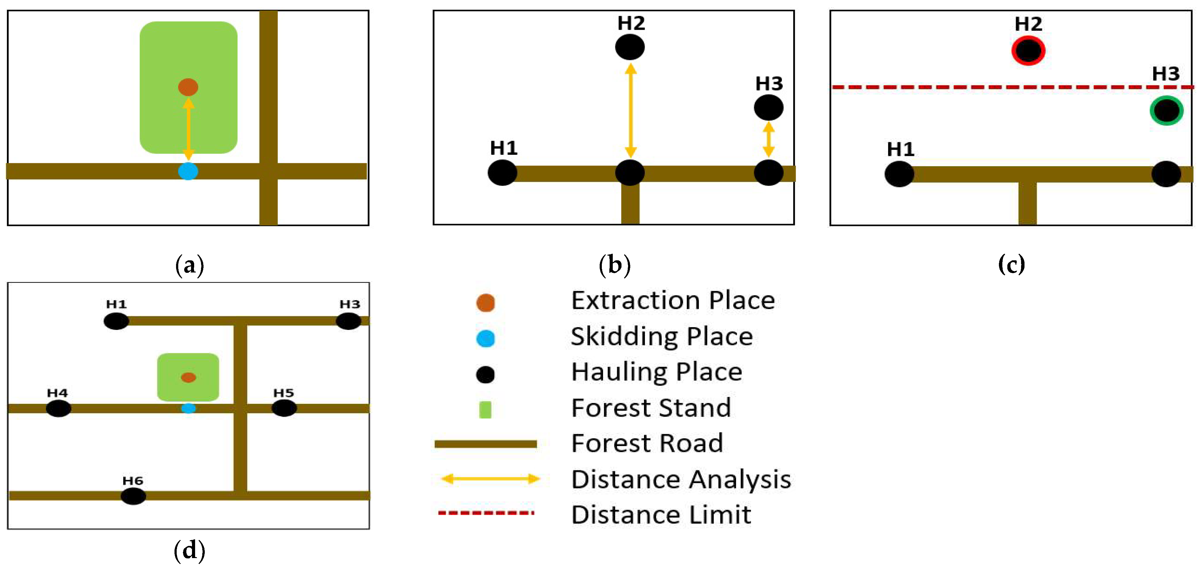
Step 1. Finding the extraction place and skidding place (Figure 2a)
The first sub-step finds the locations of the extraction places. Specifically, this sub-step creates an EP point layer that contains the geometric centers (centroids) of the target objects. These points represent the EPs, i.e., the places in the target objects from where the cut timber will be transported to the nearest forest roads along the generated pre-skidding routes. The EPs are created in the centers of the target objects as a compromise because their exact location is not defined.
The second sub-step finds the locations of the skidding places. Specifically, this sub-step creates an SP point layer that contains the nearest points on the forest roads to the Eps. These points represent the SPs, i.e., the places on the forest roads from where the cut timber will be transported to the nearest hauling places along the forest roads. The SPs are created at the nearest point on the forest road to the EPs as a compromise because their exact location is not defined.
Figure 2. (a) Step 1: The first sub-step creates points representing the extraction places (EPs) located in the geometric centers of the target objects (e.g., forest stands, cells, tree crowns, buildings), and the second sub-step creates points representing the skidding places (SPs) located at the nearest points on the forest roads to the EPs. (b,c) Step 2: The first sub-step finds the topologically correct positions of the hauling places (HPs) on the forest roads, and the second sub-step finds the correct set of HPs. For example, Figure 2b includes a set of three original HPs (H1, H2, H3). Since only one HP (H1) has overlay with the forest road, the first sub-step finds the nearest points on the forest roads for the remaining two HPs (H2, H3) and creates a temporary point layer consisting of all three HPs (H1, H2, H3) with topologically correct positions. However, this layer may still contain outlying HPs. The second sub-step, therefore, uses the user-defined distance limit (default is 15 m) for the selection of relevant HPs (Figure 2c). Since one HP (H2) exceeds this distance limit, the final point layer consists of only two HPs (H1, H3). (d) The network dataset consists of topologically correct and relevant objects.
Forests 14 00907 g002
Step 2. Finding the position of the relevant hauling place on the forest road (Figure 2b,c)
The first sub-step finds the locations of the hauling places. Specifically, this sub-step creates a temporary HP1 point layer that contains the nearest points on the forest roads to the input hauling places. The HP1 is created to ensure the topologically correct position of the hauling places. Even if the position of the hauling places is defined, the related layers (i.e., hauling place and forest road) may not share coincident geometry (e.g., there is no overlay between the hauling places and the forest roads).
The second sub-step finds the relevant hauling places. Specifically, this sub-step creates an HP2 point layer that contains selected hauling places from HP1, whose distance from the forest roads does not exceed a user-defined distance limit (the default is 15 m). The HP2 is created to ensure the correct set of hauling places. Even if the position of the hauling places is defined, the related layer (i.e., hauling place) may contain irrelevant points (e.g., hauling places from different areas of interest).
Step 3. Finding the nearest hauling place to the skidding place (Figure 3)
The first sub-step finds, at maximum, the three nearest hauling places to the skidding place. Specifically, this sub-step uses a relatively undemanding geospatial technique for the calculation of the straight-line distance between the skidding places and all HP2s. Moreover, the user-defined distance limit (the default is 2000 m) will ensure that only relevant HP2s are searched for this calculation, avoiding potentially endless searches. Finally, the sub-step selects, at maximum, the three HP2s with the lowest distance values and marks them as the three nearest hauling places to the related skidding places (HP3). In this way, a further and relatively demanding sub-step will only take place for a maximum of three hauling places that have the smallest direct distance to the related skidding place and which are located within the limit of the maximal straight-line distance from this skidding place.
The second sub-step finds the nearest hauling place to the skidding place. Specifically, this sub-step uses Dijkstra’s algorithm for the calculation of the shortest distance between the skidding places and all HP3s. Here, each node (i.e., vertexes on the forest roads) is assigned a tentative cost, which is initially “zero” for the source node (i.e., skidding place) and “infinity” for all other nodes. The algorithm then starts from the source node and visits all outgoing arcs (i.e., the parts of forest roads between vertexes) from there. For each such outgoing arc, it checks whether, via this arc, it can reach the node at the other side of the arc at a lower cost than assigned to that node so far. If yes, its tentative cost is updated to the new, lower cost. This procedure is iterative until the target node (i.e., HP3) is settled. In this way, all three hauling places from HP3 acquire a value of the shortest distance to the related skidding places along the road network. Finally, the sub-step selects one hauling place from HP3 with the lowest distance value and marks it as the nearest hauling place to the related skidding place (HP4).
Figure 3. (a) Step 3: The first sub-step calculates a straight-line distance between the skidding places (SP) and all hauling places (HP). Moreover, a user-defined distance limit (the default is 2000 m) will ensure that only relevant HPs are searched for this calculation, avoiding potentially endless searches. Finally, this sub-step selects, at maximum, the three HPs with the lowest distance values and marks them as the three nearest HPs to the related SPs. For example, Figure 3a includes five HPs (H1, H3–H6). Even if four HPs (H1, H4–H6) meet the distance limit, only the three nearest HPs (H4–H6) are relevant for the next sub-steps. (be) The second sub-step uses Dijkstra’s algorithm for the calculation of the shortest distance between the SPs and all relevant HPs selected within the first sub-step. Finally, this sub-step selects one HP with the lowest distance value and marks it as the nearest HP to the related SP. For example, Figure 3e shows that the nearest HP to the related SP is H5.
Forests 14 00907 g003
Step 4. Measuring transportation distance (Figure 4)
The first sub-step calculates the PSD at the 2D or 3D levels. Specifically, this sub-step finds related layers (i.e., EP and SP) in the network dataset and calculates the PSD. The PSD at the 2D level is calculated when a terrain model is not available. The PSD at the 3D level is calculated when a terrain model is available.
The second sub-step calculates the SD at the 2D or 3D levels. Specifically, this sub-step finds related layers (i.e., SP and HP4) in the network dataset and calculates the SD. The SD at the 2D level is calculated when a terrain model is not available. The SD at the 3D level is calculated when a terrain model is available.
The third sub-step calculates the PTD at the 2D or 3D levels. Specifically, this sub-step calculates the PTD by summarizing the PSD and SD.
Figure 4. (a) Step 4: The first and second sub-steps find related layers in the network dataset and calculate the pre-skidding distance (PSD) and skidding distance (SD). While the calculation of the two-dimensional distance is the default, the three-dimensional distance is calculated when a terrain model is available. (b) The third sub-step calculates the primary transportation distance (PTD) by summarizing the two-dimensional or three-dimensional PSD and SD.
Forests 14 00907 g004

2.2. Applicability Assessment of the Geoprocessing Tool

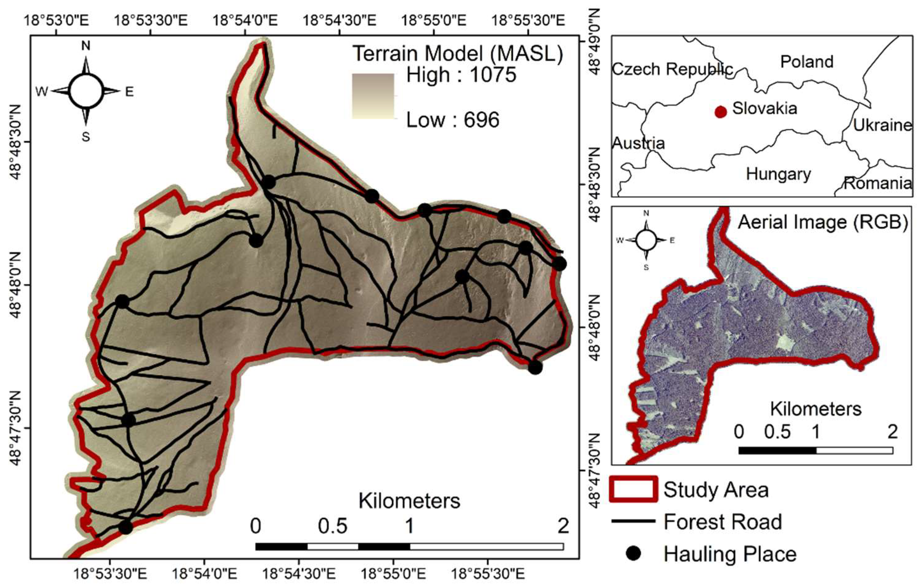
A case study was conducted in the territory of a forest unit managed by State Enterprise Forests of the Slovak Republic (approx. 48°48′ N, 18°54′ E). The total area is 400 ha, and forests occupy 391 ha in this area. The elevation reaches between 696 and 1075 m above sea level.
A source geodatabase included four types of target objects (i.e., 366 forest stands, 10,341 square cells, 7220 hexagon cells, and 83,120 tree crowns) and a digital terrain model with a resolution of 0.5 m.
Additional data were collected during the leaf-off season in 2021 through a field survey. This survey included the localization of forest roads and hauling places using a Topcon FC-25A field controller embedded with a mapping-grade global navigation satellite system (GNSS) receiver (Table 1). In this way, a total of 186 parts of forest roads (58,585 m) and 18 hauling places were localized.
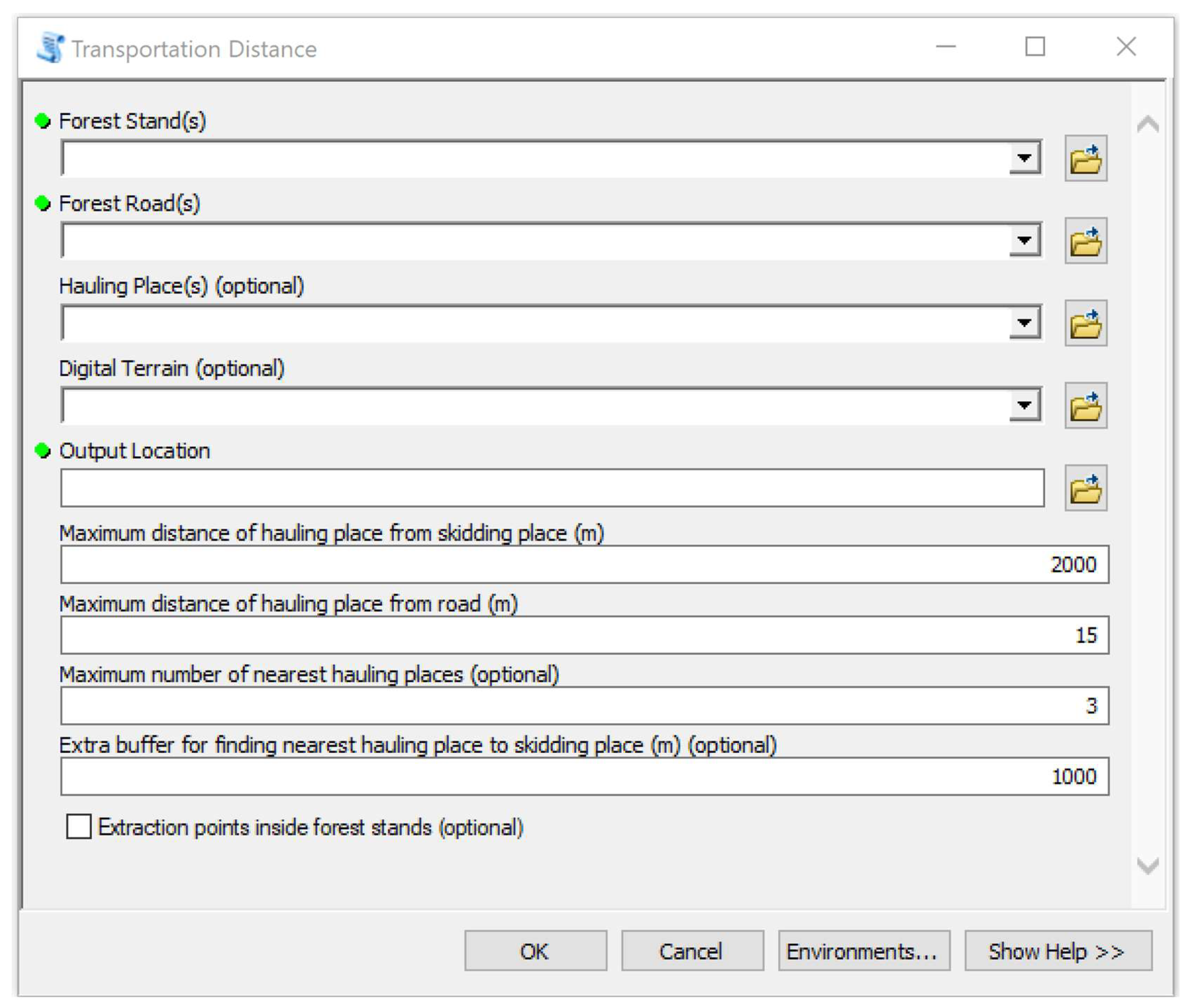
Available data from the geodatabase and field survey were imported into the network dataset in ArcGIS Desktop 10.6 (Figure 5). Finally, the PSD, SD, and PTD at the 2D and 3D levels were calculated using the TraDis tool by the high-performance workstation HP Z6 G4 (Table 2). This calculation was performed for all four types of available target objects (i.e., forests, squares, hexagons, and crowns). We used the default parameters of the user-defined limits. Specifically, (1) the maximum distance of the hauling place from the skidding place was 2000 m, (2) the maximum distance of the hauling place from the forest roads was 15 m, and (3) the maximum number of nearest hauling places to the skidding place was 3.
Table 1. Technical specifications for mapping-grade receiver Topcon FC-25A.
AttributeSpecifications
GNSS (chipset, channels, antenna)SiRFstar III GPS L1, 20, Internal
Horizontal accuracy (RMS)DGPS: 1–3 m, Point positioning: 5 m
Processor (frequency)533 MHz
Memory (capacity and type)256 MB SDRAM, 2 GB Flash
SystemMicrosoft Windows Mobile 6.5
Note: The technical specifications of the global navigation satellite system (GNSS) have a significant influence on the position accuracy of the input files related to the calculation of the transportation distance.
Table 2. Technical specifications for high-performance workstation HP Z6 G4.
AttributeSpecifications
Processor (frequency, cache, cores)2.3/3.9 GHz, 22 MB, 16
Memory (capacity, speed)128 GB RAM, 2666 MHz
Graphic card (memory, speed, cores)16 GB, 1620 MHZ, 48
Internal storage (capacity and type)1 TB SSD, 4TB HDD, 4 TB HDD
SystemMicrosoft Windows 10 Pro
Note: The technical specifications of the workstation have a significant influence on the time consumption of the calculation of the transportation distance.
Figure 5. Study area, including terrain model and aerial image.
Forests 14 00907 g005

3. Results

3.1. Geoprocessing Tool

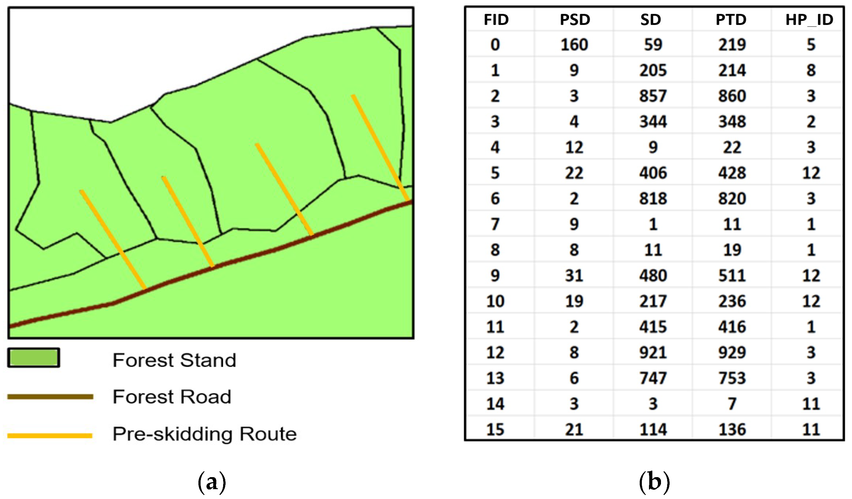
The TraDis is a geoprocessing tool designed for ArcGIS Desktop to calculate the PSD, SD, and PTD at the 2D or 3D levels (Figure 6). This tool can be executed using ArcToolbox or ArcCatalog through single-processor and multi-processor systems. The results of the calculations include two vector layers (Figure 7a). The first layer contains lines representing the generated pre-skidding routes with identifiers of the target objects. The second layer contains polygons representing these target objects with all the original records. However, the attribute table of this layer also includes new columns containing the PSD, SD, and PTD, as well as the identifier of the nearest HP (Figure 7b).

3.2. Applicability of the Geoprocessing Tool

The time consumption for the calculation of the transportation distances is shown in Table 3. The calculation of the 2D distances took ca. 1 min for 366 forests, ca. 21 min for 10,341 squares, ca. 13 min for 7220 hexagons, and ca. 9 h for 83,120 crowns. The calculation of the 3D distances took an average of 63 ± 10% longer. These calculation times were influenced mainly by the size and shape of the target objects. The influence of the number of target objects and their dimensions was less pronounced. Specifically, while the relative variability in the calculation time related to the number of target objects (i.e., duration vs. count) achieved a value of 66.8%, in the case of the area in hectares (i.e., duration vs. area), this variability was 166.3%.
The transportation distances at the 2D and 3D levels are summarized in Table 4 and Table 5, respectively. With regard to the target objects, the 2D distances were found between 43 and 46 m for pre-skidding, 430 and 480 m for skidding, and 472 and 526 m for primary transportation. The 3D distances were between 44 and 48 m for pre-skidding, 433 and 485 m for skidding, and 478 and 532 m for primary transportation. In this context, the PSD was influenced mainly by the dimension, and the SD by the types of target objects. Specifically, while the PSD at the 3D level was 3.6% greater than the PSD at the 2D level, in the case of the SD, the increase was only 0.9%. On the other hand, the relative levels of variability in the PSD and SD related to the different target objects were 3.4% and 4.9%, respectively.
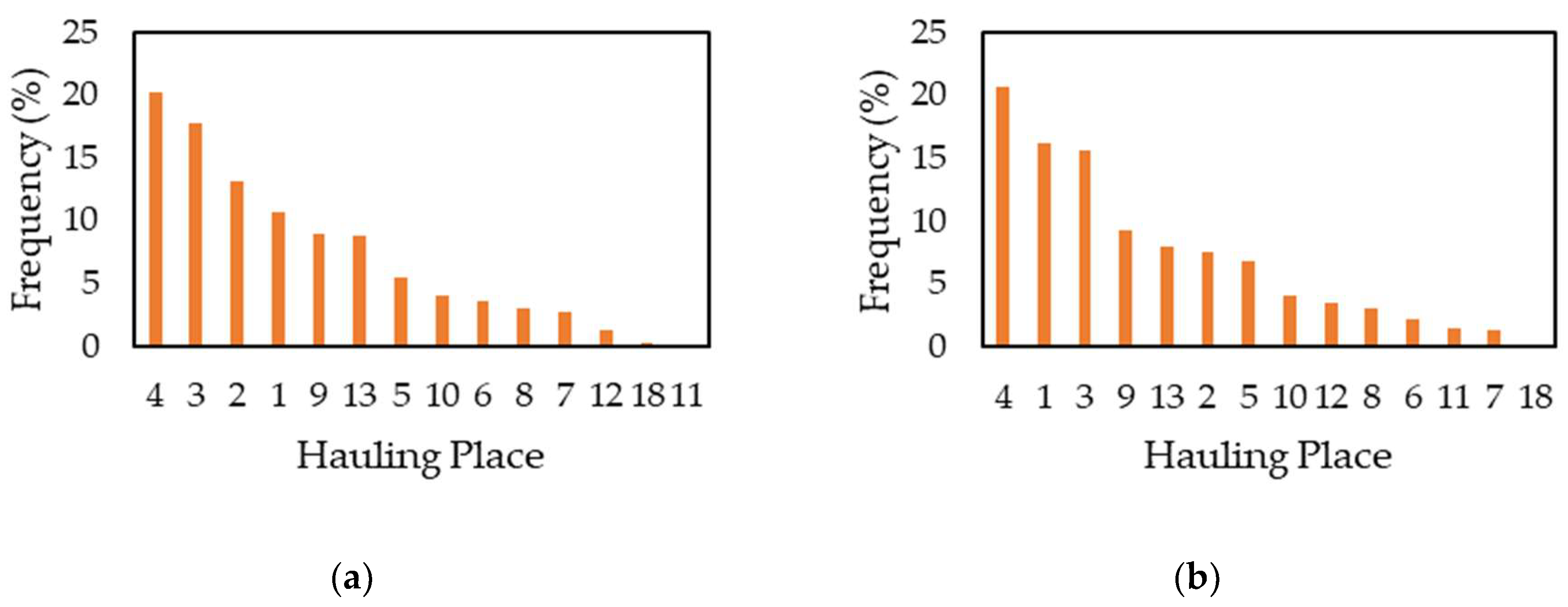
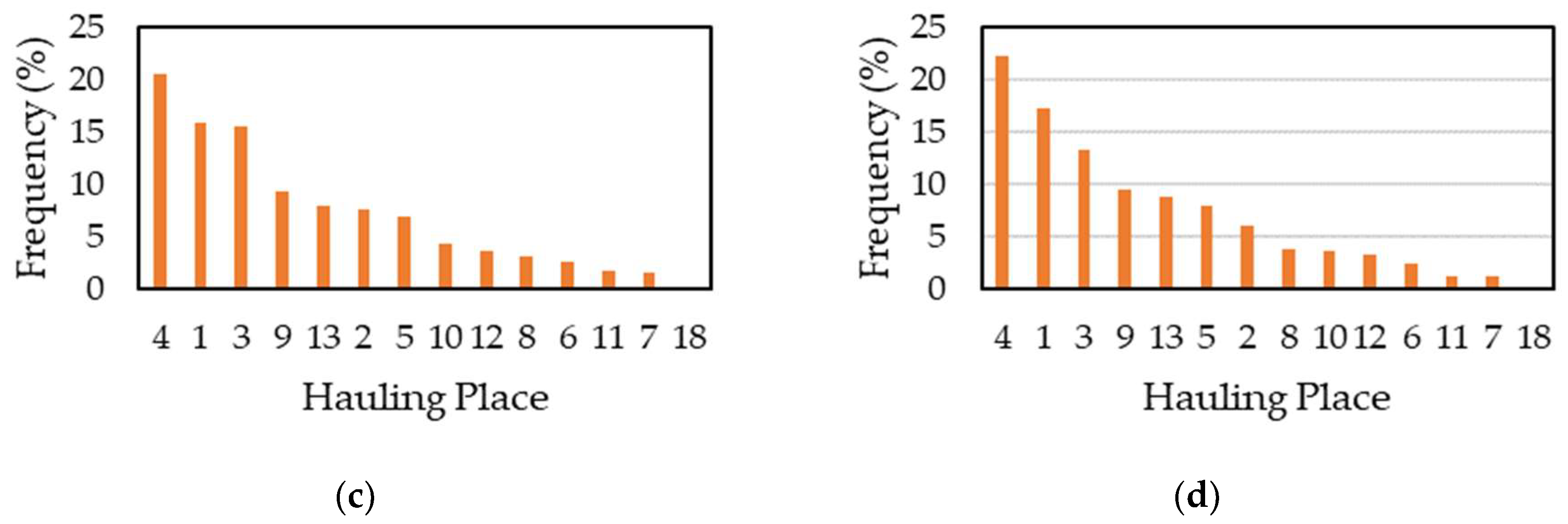
The relative levels of the suitability of the individual hauling places for wood transportation from different target objects are shown in Figure 8. Here, no differences were found between the 2D and 3D calculations. The greatest suitability was achieved at hauling places H4, H3, H1, and H2, which were the nearest for approximately 60% of target objects.
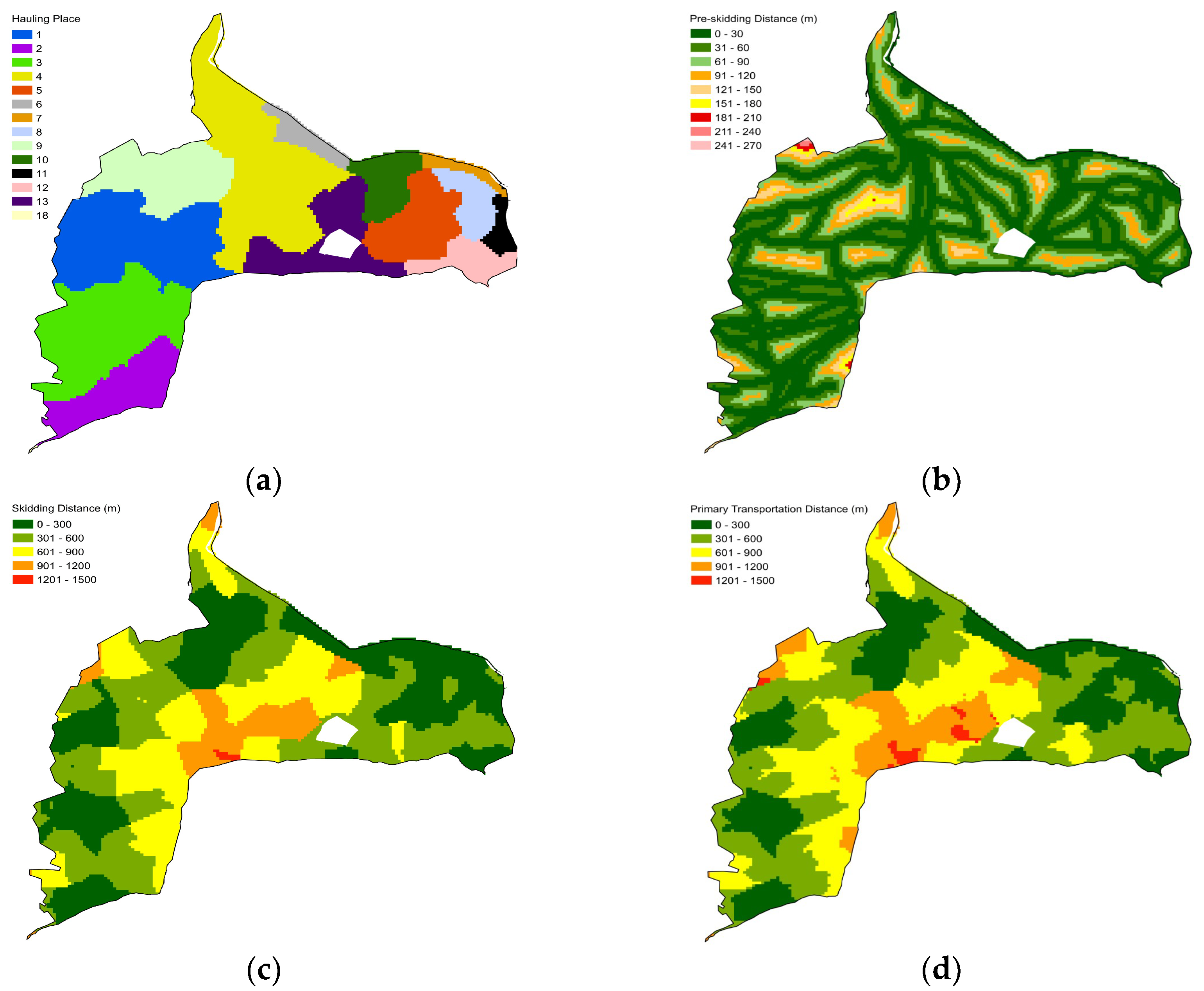
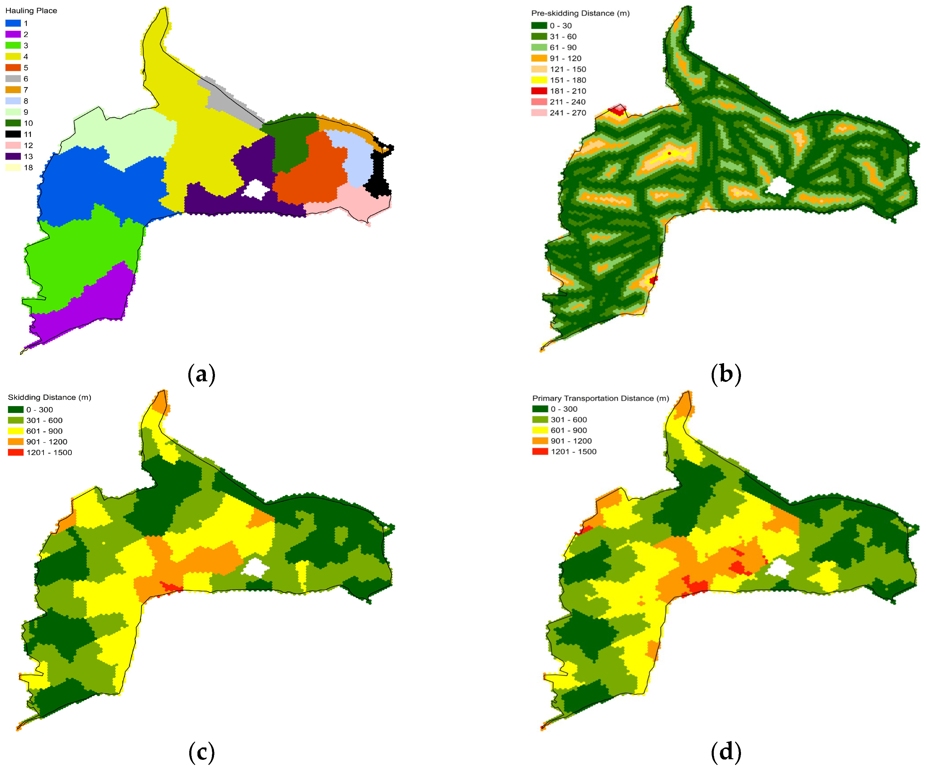
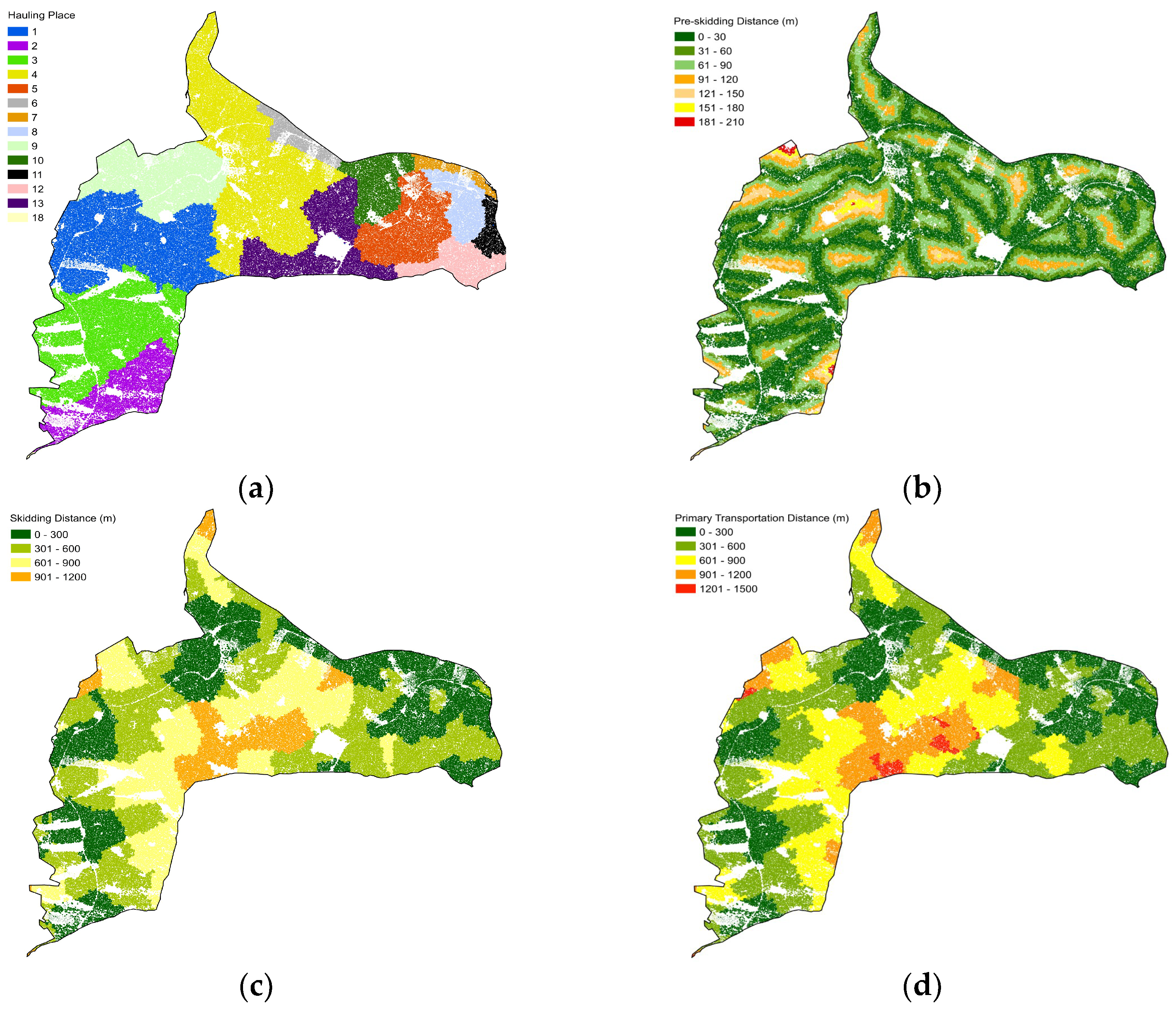
The maps represent the suitability of individual hauling places for wood transportation, and all transportation distances at the 2D level are shown in Figure 9, Figure 10, Figure 11 and Figure 12. Here, each target object (i.e., forest stands, squares, hexagons, and tree crowns) includes related values of the PSD, SD, PTD, and the identifier of the nearest hauling place. While maps with forests represent the standard data source for forest management, maps with other target objects (i.e., squares, hexagons, and crowns) provide more detailed information related to wood transportation.

4. Discussion

The motivation for the development of a geoprocessing tool for the calculation of primary wood transportation distances was mainly due to the following points:
  • Knowledge about the distances of all parts of primary wood transportation is essential for sustainable forest management [4]. Here, an appropriate structure of road networks with minimal transportation distances increases the efficiency of forest activities and decreases the negative impact on the environment [5,6,7]. Moreover, transportation distance is a key factor in the management of forest protection against fire and flood events [8,9,10];
  • The calculation of primary wood transportation distances based on geospatial methods or tools allows for the use of a comprehensive database and an automated calculation, and the resulting distance is more realistic [26,27]. Nevertheless, there is no powerful single desktop geospatial tool for the calculation of the PSD, SD, and PTD at the 2D and 3D levels [35,36].

4.1. Specificity and Applicability of the Geoprocessing Tool

In contrast to other methods [28,29,32] and models [11,30,31] for the calculation of transportation distances, the geoprocessing tool TraDis provides several benefits. Specifically, an application of the TraDis tool (1) is more user-friendly because the interface (Figure 6) is intuitive, compact, and includes generally used environment and commands of ArcGIS Desktop extensions; (2) is more comprehensive because the workflow (Figure 1) covers all parts of primary wood transportation (i.e., pre-skidding, skidding) and both levels of dimension (i.e., 2D, 3D); (3) is more efficient because the third algorithm step (Figure 3) includes unique geospatial processes focused on reducing the calculation time and ensuring the correct topology of input/output data; and (4) is more accurate because the fourth algorithm step (Figure 4) uses only topologically correct data and the optional 3D data from the digital terrain model. Moreover, the workflow includes Dijkstra’s algorithm (Step 3), which is a powerful computer solution for network analysis. While most forestry applications use this shortest path algorithm to find the optimal position of roads [37,38] or log yards [39], the TraDis tool uses Dijkstra’s algorithm to find the nearest hauling place to the related skidding place (Step 3).
These specific features of the TraDis tool were verified through a case study. The study area and data included 391 ha of forest stands; 58 km of forest roads; 18 hauling places; and various target objects, including 366 forest stands, 10,341 square cells, 7220 hexagon cells, and 83,120 tree crowns. The results show that the PSD was influenced mainly by the dimensions, and the SD by the type of target object (Table 4 and Table 5). This is because, while the pre-skidding routes were located on the original surface of the forest terrain, the surface of the forest roads had corrected for maximal and minimal slopes. Specifically, the ratio between the 3D and 2D distances achieved a value of 1.04 for the PSD and 1.01 for the SD. Although this relationship was expected and confirmed [11], other studies with respect to terrain topography defined this ratio between 1.2 and 4.2 [13,16,40,41]. The results also show that the calculation time was influenced mainly by the size as well as the shape of the target objects, and subsequently, by the number of target objects and their dimensions (Table 3). Specifically, while there was the ability to calculate the 2D distance for six forests, eight cells, and three crowns in one second, the calculation time of the 3D distance was 1.6 times longer. Although there have been no similar studies to compare these results, knowledge about these relationships is very important for a wider application of the TraDis tool.

4.2. Future Improvement of the Geoprocessing Tool

The first weakness of the current version of the TraDis tool is its exclusive relationship with the commercial software application ArcGIS Desktop. Moreover, the calculation of distances at the 3D level requires a specific ArcGIS extension. A future improvement could therefore include the modification of the algorithm to other, even freely available, geospatial environments. For example, its modification for the QGIS [42] or GRASS GIS [43] environment seems promising. Both of these environments also use the Python programming language, and both allow for creating additional extensions and contain tools with the same or similar functionality as the basic ArcGIS modules used. In addition, it would be possible to use the specific tools of these environments for network analysis to speed up calculations or adapt calculations for 3D analysis, as both environments support 3D vector format. Finally, this improvement would make the calculation of transportation distances more available.
The second weakness of the current version of the TraDis tool is that it does not take into account the uphill/downhill transportation as well as the category of road. A future improvement could therefore include the implementation of additional conditions into the algorithm. Thus, the relationship between the extraction place and the skidding place would not only be based on the near distance but also on the slope and category of the road. Finally, this improvement would make the calculation of the transportation distance more realistic.

5. Conclusions

This study presents a workflow and applicability of the authors’ geoprocessing tool TraDis, which is designed for the calculation of primary wood transportation distances. The following are the key findings:
  • The TraDis tool was developed as an extension for ArcGIS Desktop to calculate the PSD, SD, and PTD at the 2D or 3D levels. The workflow includes four steps: (1) finding the extraction place and skidding place, (2) finding the position of the relevant hauling place on the forest road, (3) finding the nearest hauling place to the skidding place, and (4) measuring the transportation distance;
  • The TraDis tool allows for the calculation of transportation distances for various target objects (e.g., forest stands, cells, tree crowns, or buildings). The case study presented herein showed that the calculation of 2D distances for different numbers and types of target objects could take from 0.2 s ha−1 to 81.9 s ha−1, and the 3D calculation increased this time consumption by 63 ±10%. Moreover, the PSD and SD at the 3D level could be 3.6% and 0.9% greater than these distances at the 2D level, respectively;
  • The future improvement of the TraDis tool could include (1) the modification of the algorithm to other, even freely available, geospatial environments and (2) the implementation of additional conditions (i.e., slope, category of the road) into the algorithm. These future improvements would make the calculation of transportation distances more available and realistic.

Author Contributions

Conceptualization, I.S.; methodology, I.S.; software, I.B.; validation, I.S., resources, I.S.; writing—original draft preparation, I.S.; writing—review and editing, I.S. and I.B.; project administration, I.S.; funding acquisition, I.S. All authors have read and agreed to the published version of the manuscript.

Funding

This research and the APC were funded by the Slovak Research and Development Agency in the framework of the project “Development of advanced geospatial technologies for multiscale monitoring of forest ecosystems” (APVV-19-0257).

Data Availability Statement

Not applicable.

Conflicts of Interest

The authors declare no conflict of interest.

References

  1. Schiess, P.; Krogstad, F. Forest Harvest and Transportation. In Fishes and Forestry: Worldwide Watershed Interactions and Management; Northcote, T.G., Hartman, G.F., Eds.; Wiley-Blackwell: Hoboken, NJ, USA, 2007; pp. 193–215. [Google Scholar]
  2. Çağlar, S.; Altunel, A.O. The Effects of Primer Transport Techniques on Raw Wood Materials in Turkey. In Proceedings of the International Forest Products Congress, Trabzon, Turkey, 26–29 September 2018; pp. 818–827. [Google Scholar]
  3. Koirala, A.; Kizha, A.R.; De Hoop, C.F.; Roth, B.E.; Han, H.-S.; Hiesl, P.; Abbas, D.; Gautam, S.; Baral, S.; Bick, S.; et al. Annotated Bibliography of the Global Literature on the Secondary Transportation of Raw and Comminuted Forest Products (2000–2015). Forests 2018, 9, 415. [Google Scholar] [CrossRef]
  4. Shadbahr, J.; Bensebaa, F.; Ebadian, M. Impact of forest harvest intensity and transportation distance on biomass delivered costs within sustainable forest management—A case study in southeastern Canada. J. Environ. Manag. 2021, 284, 112073. [Google Scholar] [CrossRef]
  5. Palander, T.; Borz, S.A.; Kärhä, K. Impacts of Road Infrastructure on the Environmental Efficiency of High Capacity Transportation in Harvesting of Renewable Wood Energy. Energies 2021, 14, 453. [Google Scholar] [CrossRef]
  6. Borz, S.A.; Crăciun, B.C.; Marcu, M.V.; Iordache, E.; Proto, A.R. Could timber winching operations be cleaner? An evaluation of two options in terms of residual stand damage, soil disturbance and operational efficiency. Eur. J. For. Res. 2023, 1–17. [Google Scholar] [CrossRef]
  7. Palander, T.; Haavikko, H.; Kortelainen, E.; Kärhä, K. Comparison of Energy Efficiency Indicators of Road Transportation for Modeling Environmental Sustainability in “Green” Circular Industry. Sustainability 2020, 12, 2740. [Google Scholar] [CrossRef]
  8. Mohammadi, Z.; Lohmander, P.; Kašpar, J.; Marušák, R. The effect of road networks on the forest wildfires size. In Proceedings of the EGU General Assembly 2021, Online, 19–30 April 2021. [Google Scholar]
  9. Marche, J.; Lettenmaier, D. Effects of Forest Roads on Flood Flows in the Deschutes River, Washington. Earth Surf. Process. Landf. 2001, 26, 115–134. [Google Scholar] [CrossRef]
  10. Ruiz-Villanueva, V.; Bodoque, J.; Díez-Herrero, A.; Bladé, E. Large Wood Transport as Significant Influence on Flood Risk in a Mountain Village. Nat. Hazards 2014, 74, 967–987. [Google Scholar] [CrossRef]
  11. Enache, A.; Pentek, T.; Ciobanu, V.; Stampfer, K. GIS based methods for computing the mean extraction distance and its correction factors in Romanian mountain forests. Sumar. List. 2015, 139, 35–46. [Google Scholar]
  12. Matthews, D.M. Cost Control in the Logging Industry; McGraw-Hill Book Company Inc.: New York City, NY, USA, 1942; pp. 1–374. [Google Scholar]
  13. Segebaden, G. Studies of cross-country transport distances and road net extension. Stud. For. Suec. 1964, 18, 1–70. [Google Scholar]
  14. Klč, P.; Žáček, J.; Sotorník, M. Accessibility of the forests in the Czech Republic through forest transportation network. Lesn. Časopis—For. J. 2006, 52, 297–310. [Google Scholar]
  15. Tománek, J.; Volný, C. Examination of current access to forest and projected finishing of main logging road network in selected area of Beskids. Lesn. Časopis—For. J. 2009, 55, 409–417. [Google Scholar]
  16. Lotfalian, M.; Zadeh, E.; Hosseini, S. Calculating the correction factor of skidding distance based on forest road network. J. For. Sci. 2011, 57, 467–471. [Google Scholar] [CrossRef]
  17. Simões, D.; Cavalcante, F.S.; Lima, R.C.A.; Rocha, Q.S.; Pereira, G.; Miyajima, R.H. Optimal Forest Road Density as Decision-Making Factor in Wood Extraction. Forests 2022, 13, 1703. [Google Scholar] [CrossRef]
  18. Zhixian, Z.; Zhili, F. The Method of Calculating Average Skidding Distance. J. For. Res. 1997, 8, 47–49. [Google Scholar] [CrossRef]
  19. Backmund, F. Kennzahlen für den Grad der Erschließung von Forstbetrieben durch autofahrbare Wege. Forstwiss. Cent. 1966, 85, 342–354. [Google Scholar] [CrossRef]
  20. Dietz, P.; Knigge, W.; Löffler, H. Walderschlieβung; Verlag Paul Parey: Hamburg, Germany, 1984; p. 426. [Google Scholar]
  21. Sessions, J. Harvesting Operations in the Tropics; Springer: Berlin/Heidelberg, Germany, 2007; p. 170. [Google Scholar]
  22. Kweon, H. Comparisons of Estimated Circuity Factor of Forest Roads with Different Vertical Heights in Mountainous Areas, Republic of Korea. Forests 2019, 10, 1147. [Google Scholar] [CrossRef]
  23. Krč, J.; Košir, B. Predicting wood skidding direction on steep terrain by DEM and forest road network extension. Croat. J. For. Eng. 2008, 29, 177–188. [Google Scholar]
  24. Folegatti, B. The Application of Precision Forestry Technologies in Logging Operations. Master’s Thesis, Department of Forestry and Wildlife Sciences, Auburn University, Auburn, AL, USA, 2010; p. 138. [Google Scholar]
  25. Kulak, D.; Stanczykiewicz, A.; Szewczyk, G. Productivity and time consumption of timber extraction with a grapple skidder in selected pine stands. Croat. J. For. Eng. 2017, 38, 55–63. [Google Scholar]
  26. Abdi, E.; Majnounian, B.; Darvishsefat, A.; Mashayekhi, Z.; Sessions, J. A GIS-MCE based model for forest road planning. J. For. Sci. 2009, 55, 171–176. [Google Scholar] [CrossRef]
  27. Picchio, R.; Latterini, F.; Mederski, P.S.; Venanzi, R.; Karaszewski, Z.; Bembenek, M.; Croce, M. Comparing Accuracy of Three Methods Based on the GIS Environment for Determining Winching Areas. Electronics 2019, 8, 53. [Google Scholar] [CrossRef]
  28. Pentek, T.; Pičman, D.; Potočnik, I.; Dvorščak, P.; Nevečerel, H. Analysis of an existing forest road network. Croat. J. For. Eng. 2005, 26, 39–50. [Google Scholar]
  29. Petkovic, V.; Marčeta, D.; Ljubojevic, D.; Kuburić, J. Determination of average skidding distance using GIS. Nova Meh. Sumar. 2017, 38, 33–42. [Google Scholar]
  30. Sačkov, I.; Smreček, R.; Tucek, J. Forest transportation survey based on airborne laser scanning data and GIS analyses. GIScience Remote Sens. 2014, 51, 83–98. [Google Scholar] [CrossRef]
  31. Duka, A.; Grigolato, S.; Papa, I.; Pentek, T.; Poršinsky, T. Assessment of timber extraction distance and skid road network in steep karst terrain. Iforest—Biogeosciences For. 2017, 10, 886–894. [Google Scholar] [CrossRef]
  32. Ljubojevic, D.; Danilović, M.; Marčeta, D.; Petkovic, V. Winching Distance in Function of the Optimization of Skid Network. S.E. Eur. For. 2018, 9, 97–106. [Google Scholar] [CrossRef]
  33. Knuth, D.E. A generalization of Dijkstra’s algorithm. Inf. Process. Lett. 1977, 6, 1–5. [Google Scholar] [CrossRef]
  34. Toms, S.; O’Beirne, D. ArcPy and ArcGIS: Automating ArcGIS for Desktop and ArcGIS Online with Python, 2nd ed.; Packt Publishing: Birmingham, UK, 2017; p. 272. [Google Scholar]
  35. Heinimann, H.R. A computer model to differentiate skidder and cable-yarder based road network concepts on steep slopes. J. For. Res. 1998, 3, 1–9. [Google Scholar] [CrossRef]
  36. Amhuri, J.; Norizah, K.; Mohd Hasmadi, I.; Azfanizam, A.S. Bees algorithm for Forest transportation planning optimization in Malaysia. For. Sci. Technol. 2021, 17, 88–99. [Google Scholar]
  37. Sales, A.; Gonzáles, D.G.E.; Martins, T.G.V.; Silva, G.C.C.; Spletozer, A.G.; Telles, L.A.d.A.; Siviero, M.A.; Lorenzon, A.S. Optimization of Skid Trails and Log Yards on the Amazon Forest. Forests 2019, 10, 252. [Google Scholar] [CrossRef]
  38. Parsakhoo, A.; Mohammad, J. Determining an optimal path for forest road construction using Dijkstra’s algorithm. J. For. Sci. 2016, 62, 264–268. [Google Scholar] [CrossRef]
  39. Ricards, A. Forest Road Location Modelling with Dijkstra’s Shortest Path and ArcGIS. Ph.D. Thesis, Faculty of Natural Resources Management Lakehead University, Thunder Bay, ON, Canada, 2019; p. 36. [Google Scholar]
  40. Kanzaki, K.; Ohasi, K.; Deki, T.; Miyake, T. On capillary path systems in steep mountain areas. Int. J. For. Eng. 1990, 2, 17–21. [Google Scholar] [CrossRef]
  41. Abegg, B. Estimation of the optimal forest road density in skidder terrain. Mitteilungen 1978, 54, 101–213. [Google Scholar]
  42. QGIS Geographic Information System. Available online: http://qgis.osgeo.org (accessed on 31 January 2023).
  43. GRASS Geographic Information System. Available online: http://grass.osgeo.org (accessed on 31 January 2023).
Figure 1. The workflow for the calculation of transportation distance using the TraDis tool includes four steps: finding the extraction place and skidding place (S1), finding the position of the relevant hauling place on a forest road (S2), finding the nearest hauling place to the skidding place (S3), and measuring the transportation distance (S4).
Forests 14 00907 g001
Figure 6. Environment of the TraDis tool.
Forests 14 00907 g006
Figure 7. Outputs of transportation distance calculation using TraDis tool: (a) polygon layer of target objects (e.g., forests) and line layer of generated pre-skidding routes; (b) attribute table of target object layer including columns with values of pre-skidding distance (PSD), skidding distance (SD), primary transportation distance (PTD), and identifier of nearest hauling place (HP_ID).
Forests 14 00907 g007
Figure 8. The relative suitability of individual hauling places for wood transportation from (a) forests, (b) squares, (c) hexagons, and (d) crowns.
Forests 14 00907 g008aForests 14 00907 g008b
Figure 9. Transportation distance for 366 forest stands: (a) relationship of forests with the individual hauling places; (b) pre-skidding distance; (c) skidding distance; (d) primary transportation distance.
Forests 14 00907 g009
Figure 10. Transportation distance for 10,341 squares: (a) relationship of squares with the individual hauling places; (b) pre-skidding distance; (c) skidding distance; (d) primary transportation distance.
Forests 14 00907 g010
Figure 11. Transportation distance for 7220 hexagons: (a) relationship of hexagons with the individual hauling places; (b) pre-skidding distance; (c) skidding distance; (d) primary transportation distance.
Forests 14 00907 g011
Figure 12. Transportation distance for 83,120 tree crowns: (a) relationship of crowns with the individual hauling places; (b) pre-skidding distance; (c) skidding distance; (d) primary transportation distance.
Forests 14 00907 g012
Table 3. Time duration of transportation distance calculation in seconds per hectare.
Dimension of DistanceForestsSquaresHexagonsCrowns
Two-dimensional (s ha−1)0.163.182.0181.86
Three-dimensional (s ha−1)0.245.333.36139.25
Note: Time consumption depends on parameters of the used workstation (Table 2).
Table 4. Two-dimensional transportation distance in meters.
Category of DistanceForestsSquaresHexagonsCrowns
Pre-skidding (m)42.8 ± 37.844.5 ± 36.044.3 ± 36.246.2 ± 35.5
Skidding (m)429.6 ± 274.1480.3 ± 281.9477.4 ± 283.3479.3 ± 284.4
Primary transportation (m)472.3 ± 283.9524.9 ± 290.2521.7 ± 291.8525.5 ± 291.5
Table 5. Three-dimensional transportation distance in meters.
Category of DistanceForestsSquaresHexagonsCrowns
Pre-skidding (m)44.4 ± 39.546.0 ± 37.445.8 ± 37.747.8 ± 36.9
Skidding (m)433.4 ± 277.3484.7 ± 285.5481.9 ± 286.9483.7 ± 288.0
Primary transportation (m)477.7 ± 287.3530.7 ± 293.8527.7 ± 295.5531.5 ± 295.1
Disclaimer/Publisher’s Note: The statements, opinions and data contained in all publications are solely those of the individual author(s) and contributor(s) and not of MDPI and/or the editor(s). MDPI and/or the editor(s) disclaim responsibility for any injury to people or property resulting from any ideas, methods, instructions or products referred to in the content.