Article

Community Abundance of Resprouting in Woody Plants Reflects Fire Return Time, Intensity, and Type

1
Leverhulme Centre for Wildfires, Environment and Society, Imperial College London, South Kensington, London SW7 2BW, UK
2
School of Archaeology, Geography and Environmental Science, University of Reading, Whiteknights, Reading RG6 6AH, UK
3
Georgina Mace Centre for the Living Planet, Department of Life Sciences, Imperial College London, Silwood Park Campus, Buckhurst Road, Ascot SL5 7PY, UK
*
Author to whom correspondence should be addressed.
Forests 2023, 14(5), 878; https://doi.org/10.3390/f14050878
Submission received: 10 March 2023 / Revised: 10 April 2023 / Accepted: 18 April 2023 / Published: 24 April 2023
(This article belongs to the Section Natural Hazards and Risk Management)

Abstract

:
Plants in fire-prone ecosystems have evolved a variety of mechanisms to resist or adapt to fire. Post-fire resprouting is a key adaptation that promotes rapid ecosystem recovery and hence has a major impact on the terrestrial carbon cycle. However, our understanding of how the incidence of resprouting varies in different fire regimes is largely qualitative. The increasing availability of plant trait data and plot-based species cover data provides an opportunity to quantify the relationships between fire-related traits and fire properties. We investigated the quantitative relationship between fire frequency (expressed as the fire return time) and the proportion of resprouters in woody plants using plot data on species cover from Australia and Europe. We also examined the relationship between the proportion of resprouters and gross primary production (GPP) and grass cover, where GPP was assumed to reflect fuel loads and hence fire intensity, while grass cover was considered to be an indicator of the likelihood of ground fire and the speed of fire spread, using generalised linear modelling. The proportion of resprouting species decreased significantly as the fire return time increased. When the fire return time was considered along with other aspects of the fire regime, the proportion of resprouters had significant negative relationships with the fire return time and grass cover and a significant positive relationship with GPP. These findings demonstrate that plants with the ability to resprout occur more often where fire regimes are characterised by high-frequency and high-intensity crown fires. Establishing quantitative relationships between the incidence of resprouting and the fire return time and fire type provides a basis for modelling resprouting as a consequence of the characteristics of the fire regime, which in turn makes it possible to model the consequences of changing fire regimes on ecosystem properties.

1. Introduction

Fire is a natural process, and the type, frequency, and intensity of fire vary along climate gradients [1,2,3]. Fire significantly impacts ecosystems because it consumes variable amounts of above-ground biomass and initiates succession [4]. However, plants in fire-prone ecosystems have evolved various mechanisms to resist or adapt to fire, including fire-stimulated regeneration, post-fire flowering, fire-induced seed release (serotiny), post-fire resprouting, and thick bark [5,6,7,8]. The incidence of specific plant traits appears to be related to the frequency, intensity, and type of fire [9]. Specifically, in ecosystems with relatively infrequent fires, plants display resilience, and fire triggers enhanced recruitment through traits such as serotiny. In ecosystems with frequent but low-intensity or surface fires, species are likely to have traits that convey resistance, for example, thick bark, while in ecosystems with frequent and more intense fires, species are likely to have traits that convey resilience through rapid post-fire recovery, such as the ability to resprout.
Post-fire resprouting is the ability to regenerate rapidly after fire from underground or above-ground meristems and is one of the most widely occurring fire-adaptive traits. Resprouting allows woody plants to persist after fire, maintaining fire-adapted communities and allowing very rapid ecosystem recovery [10]. This rapid recovery has a profound impact on the terrestrial carbon cycle by promoting significant carbon sequestration [10,11,12]. However, resprouting necessarily imposes a cost in terms of carbon allocation to meristems and regrowth, and it is important to understand the conditions in which the benefits conveyed by this behaviour are sufficient to outweigh these costs.
Our current understanding of the relationships between fire regimes and resprouting is largely based on field observations at local scales. Developing a more quantitative understanding of these relationships is important to reveal the costs and trade-offs involved in this strategy. It would also provide a basis for incorporating rapid recovery through resprouting in fire-enabled vegetation models, which is currently largely ignored [12,13]. This is, in turn, important to understand how ecosystems and the terrestrial carbon cycle will be affected by future changes in climate and fire [5,6,14,15,16]. The recent increase in data availability on both plant traits [17,18,19] and plot-based species cover [20] provides an opportunity to quantify the relationships between resprouting and fire properties.
In this study, we examined the relationships between resprouting and fire properties using plot-level cover data from Australia and Europe from sPlotOpen [20]. These two regions differ in terms of their plant communities and provide a wide range of fire gradients and types. Furthermore, since there has been a considerable amount of research on fire adaptations in both regions, there have been more systematic attempts to record species-level fire-adaptive traits in regional plant trait databases such as BROT and AusTraits compared to other fire-prone regions such as North America. We first investigated the statistical relationship between fire frequency (expressed as the fire return time) and the incidence of resprouting in woody plants. We then investigated the relationships between the incidence of resprouting and other vegetation properties that influence the type of fire using generalised linear modelling (GLM). We used gross primary production (GPP) and grass cover as predictors, where GPP was considered as a measure of fuel abundance and hence fire intensity, while grass cover was considered as an indicator of the likelihood of ground fire and the speed of fire spread.

2. Methods

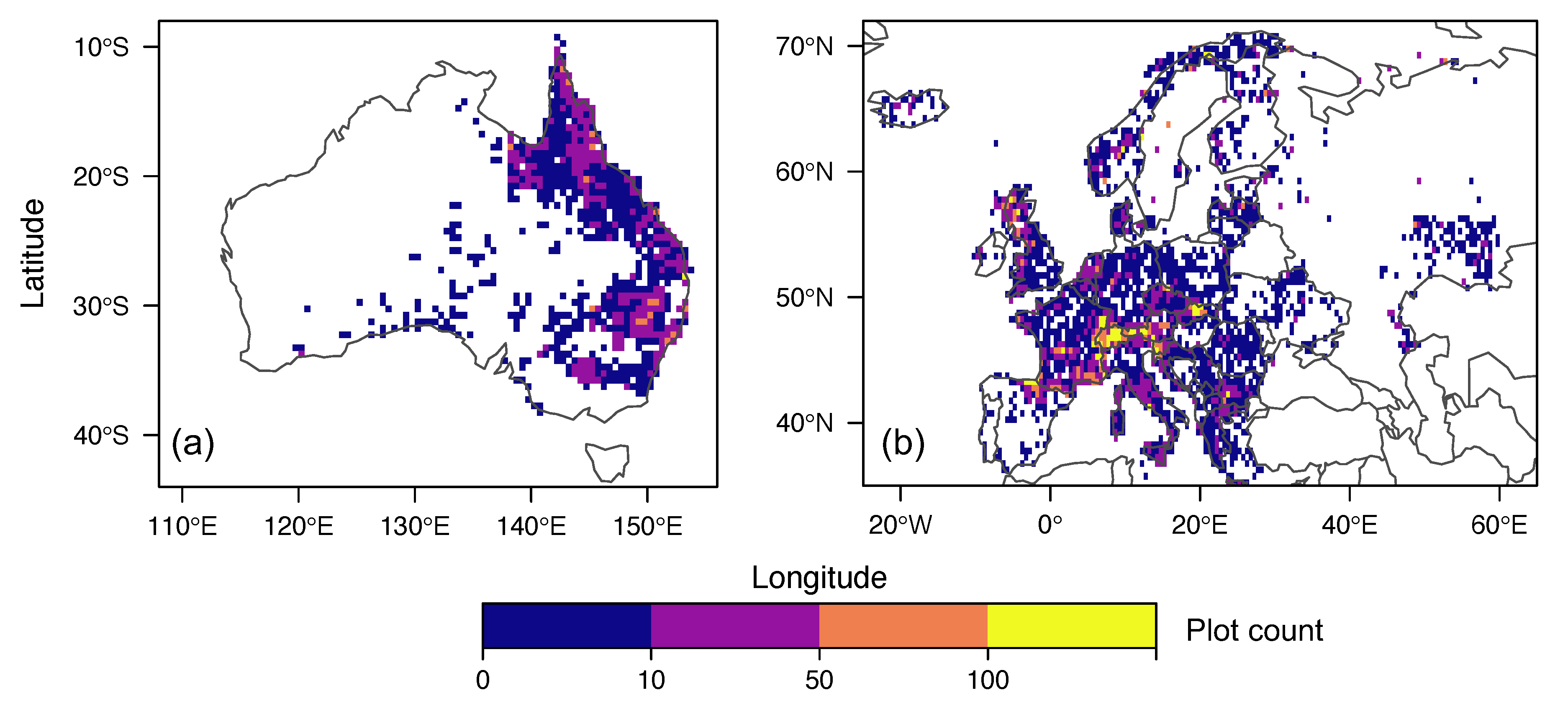
2.1. Species Cover and Resprouting Information

Information on species distributions in Australia and Europe was derived from sPlotOpen [20]. sPlotOpen provides information on the relative cover of individual species that is derived by normalising the cover of all species to 1 in each plot. We refer to this as the proportion of resprouters. We removed nested sub-plots within a larger plot in order to reduce over-sampling. The method by which species cover was recorded varied between plots in sPlotOpen. We only used plots where data were recorded for all species. Sampling methods were not always documented in Europe, but the sampling could be assumed to represent all species at undocumented sites, according to the sPlotOpen documentation; therefore, we included these plots in our sample. This yielded a combined dataset of 37,376 plots, with 8056 plots from Australia and 29,320 plots from Europe (Figure 1).
Tree and shrub species were classified into resprouters and non-resprouters using information from plant trait databases, specifically TRY (version 6, Jena, Germany), BROT, and AusTraits [17,18,19]; publications [21]; and regional expert knowledge. We investigated resprouting in woody species because their ability to resprout after fire is particularly important for the carbon cycle. We assumed that a species was a resprouter if there was one record of it resprouting across all the data sources, even if other sources recorded it as not resprouting, because the trait is facultative and the specific fire history or climate characteristics of the sampling sites can therefore impact the observations. We did not distinguish between resprouting caused by different types of disturbances (e.g., by fire, drought, or herbivory) since we assumed that the ability to resprout is an inherited trait and the ability to resprout when severely damaged means that a species could also resprout after fire. We were able to classify 1570 woody species into resprouters or non-resprouters (Table S1), representing 65% of the woody species in Australia and 38% of the woody species in Europe (Table 1).
Given the relatively high proportion of species for which no information was available about the ability to resprout (Table 1) and the potential observational bias towards recording resprouters over non-resprouters, we tested whether treating unclassified species as non-resprouters would affect the results. To do this, we calculated the proportion of resprouters in each plot in two ways: first where the proportion of resprouters was relative to the total cover of species with known responses (P1 resprouter, Equation (1)) and second where the proportion of resprouters was relative to the total cover of all woody species (P2 resprouter, Equation (2)):
P 1 r e s p r o u t e r = p r o p o r t i o n   o f   r e s p r o u t e r s p r o p o r t i o n   o f   r e s p r o u t e r s + p r o p o r t i o n   o f   n o n - r e s p r o u t e r s
P 2 r e s p r o u t e r = p r o p o r t i o n   o f   r e s p r o u t e r s p r o p o r t i o n   o f   a l l   w o o d y   s p e c i e s
where the proportion was calculated as the sum of the relative cover data of all the species in each category in each plot.

2.2. Fire Return Interval

The fire return interval (FRI) was estimated using three remote-sensing fire products: MODIS MCD64CMQ, FireCCI51, and FireCCI10LT. The Moderate Resolution Imaging Spectroradiometer (MODIS) Collection 6 Burned Area product [22,23] is the most widely used fire product, and it covers the period from 2001 to 2020. The European Space Agency’s Climate Change Initiative FireCCI version 5.1 (FireCCI51) [24] is better at recording small fires and covers the period from 2001 to 2020. FireCCI10LT [25] covers a longer time period (36 years) than the other products because it makes use of AVHRR-LTDR data. The record starts in 1982 and ends in 2018, although there are limited data for 1994; this year was therefore omitted. All three products have a spatial resolution of 0.25°. To estimate the FRI from each product, we first calculated the total burnt area fraction for each year and then derived an average total burnt area fraction over all available years. The FRI was estimated as the reciprocal of the average total burnt area fraction [26].
There are differences between the burnt areas retrieved from different remote-sensing products (see, e.g., [27]), and since they cover different lengths of time, there can also be differences in the FRI estimated from each product. In order to assess the robustness of our estimates of the FRI, we used a model-based prediction of the burnt area fraction [28] to calculate an independent measure of the FRI. Model outputs for the interval from 2010 to 2015 were obtained at a 0.5° resolution, and the FRI was estimated as the reciprocal of the average total burnt area fraction over these five years.
We extracted the estimated FRI for each of the sPlotOpen plots according to their geographic location information. We truncated the FRI estimates to <5000 years because longer estimates are artefacts of the short time interval recorded by the remotely sensed products and the highly stochastic nature of fire.

2.3. Analysis of Relationships between the Incidence of Resprouters and Fire Properties

We first investigated the relationship between the FRI and the incidence of resprouting. The FRI was log-transformed before the analysis to reduce skewness. We used box plots to display the patterns in different categories of FRI and tested the significance of the mean and median differences between the FRI categories using the pairwise t-test and the non-parametric Kruskal–Wallis test. We compared the combined data from Australia and Europe and the data from each continent separately using the four different estimates of the FRI.
The incidence of resprouting could be affected by other aspects of the fire regime, such as the fire intensity, the speed of fire spread, and whether an event was a ground fire or crown fire [7,29,30]. The radiative power of fire has been used as a measure of fire intensity [31], but it represents the intensity at the flaming front and is thus difficult to use at the plot level. Here, we used GPP as a surrogate for intensity based on the assumption that high-intensity fires occur in regions with large amounts of fuel [3,28]. The abundance of herbaceous vegetation is a primary control of whether events are crown fires or ground fires and also determines the speed of fire spread [6]. We used grass cover as a surrogate index for herbaceous vegetation.
The GPP data were derived from the P-model [32,33,34], an optimality-based light-use efficiency model that simulates GPP as a function of the atmospheric pressure, the atmospheric CO2 concentration, the air temperature, the vapor pressure deficit (VPD), the incident photosynthetic photon flux density (PPFD), the fraction of incident PPFD absorbed by vegetation (fAPAR), the soil moisture (θ), and the C3/C4 vegetation fraction. The model was run using the atmospheric pressure calculated using elevation data from WFDEI [35], climate data obtained from CRU TS4.04 [36], fAPAR from GIMMs 3 g [37], and the C3/C4 vegetation fraction from [38]. The P-model has been shown to produce reliable estimates of GPP compared to site-based flux tower measurements [32,33,34] while requiring the calibration of only two parameters. Thus, it provides more transparent estimates than other GPP products. Simulated monthly GPP values at a 0.5° resolution over the period from 2001 to 2016 were summed to derive the annual total GPP. Since the year-to-year variation in GPP was small, we used the mean annual total GPP over the 16-year interval. We converted the data to 0.25° via bilinear interpolation for consistency with the FRI estimated using the remotely sensed products. The grass cover was obtained from ESACCI LC data [39]. The raw data had a 300 m spatial resolution on an annual basis from 2001 to 2016. We used the fractional grass cover to calculate the mean grass cover over these years and then converted this to 0.25° via bilinear interpolation. The year-to-year variations over the 16-year interval were also examined for grass cover. GPP and grass cover data were extracted for each of the sPlotOpen plots according to their geographic locations.
We investigated the relationships between the FRI, GPP, and grass cover using a binomial generalised linear model (GLM). GLMs are suitable for analyses when the response variables have highly non-Gaussian error distributions and allow quantification of the independent effects of multiple predictors, even when they are partially correlated with one another [40,41]. We applied log-transformations to GPP and the FRI to reduce skewness. We calculated the variance inflation factor (VIF) for each variable in the GLM to ensure that the regression coefficients were not inflated due to multicollinearity [42]. We used partial residual plots, which showed the effect of each predictor when the others were held constant [43], to understand the relationship between each predictor and the proportion of resprouters.
To test the impact of having incomplete information about the resprouting ability of individual species, we examined the robustness of the GLM-derived relationships across plots with different proportions of known cover using sPlotOpen plots with <25%, <50%, <75%, and <100% relative known cover of resprouters and non-resprouters in the total number of woody species.

3. Results

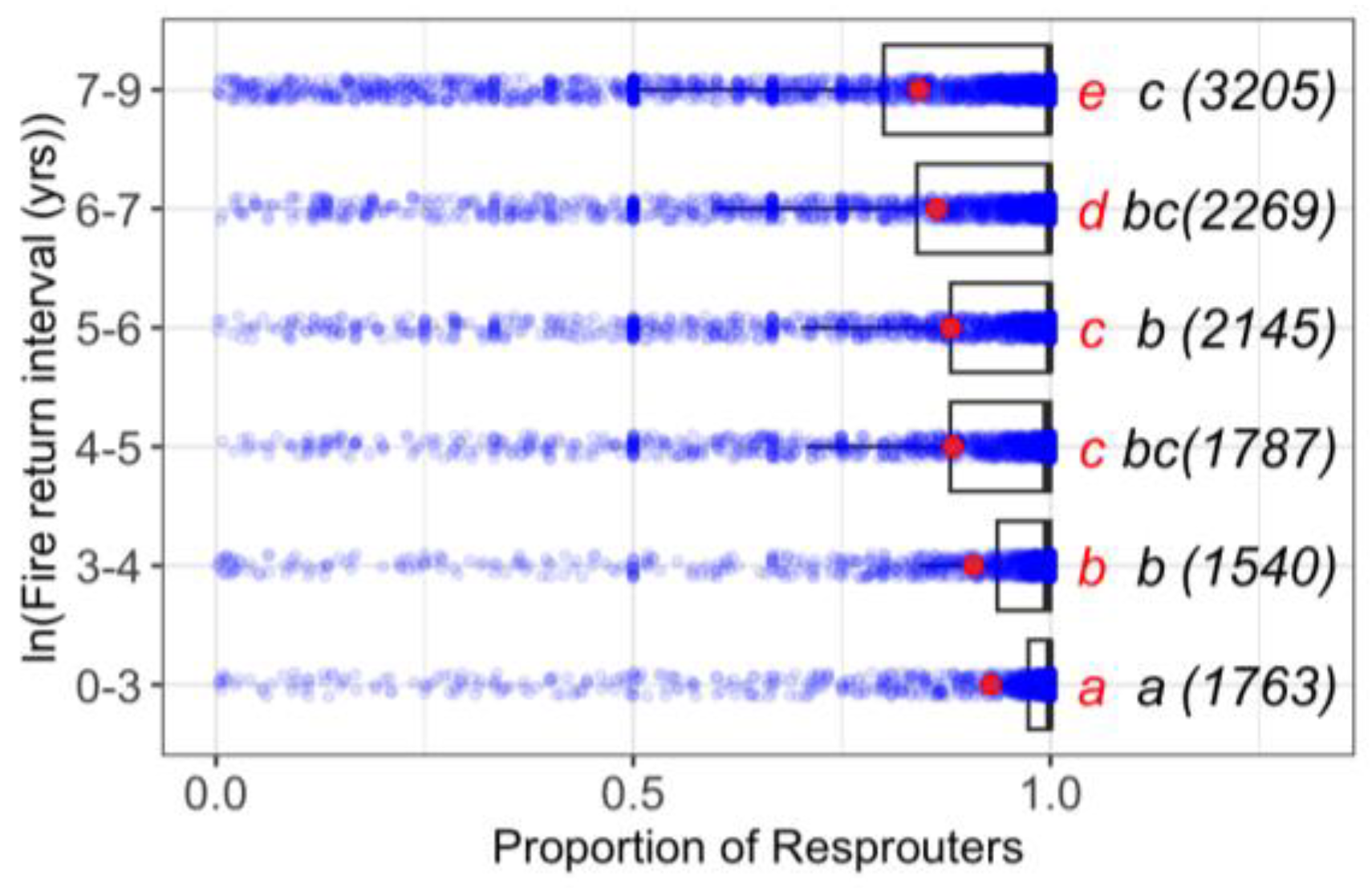
3.1. Relationship between the Fire Return Interval and the Incidence of Resprouting

The incidence of resprouters decreased as the FRI increased (Figure 2). Both the mean and median values of the different categories were significantly different from one another. This trend was also seen when the plots from each continent were considered separately (Figure S1) and was robust when different datasets were used to derive the FRI (Figure S2).

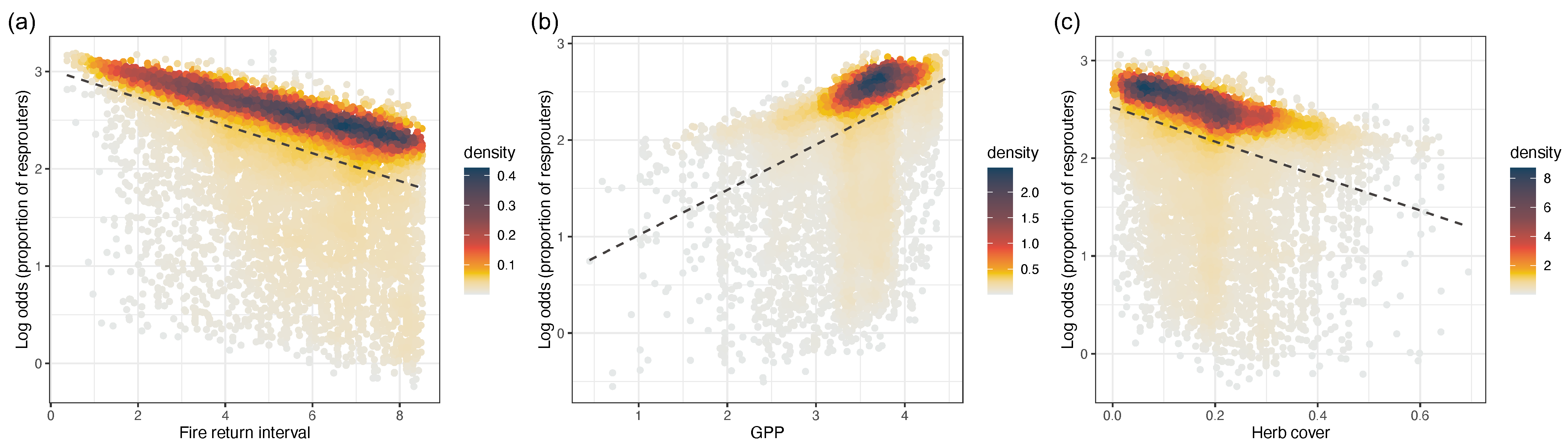
3.2. Relationships between the Incidence of Resprouting, GPP, and Grass Cover

The three predictor variables used in the GLM were not significantly correlated, with pairwise correlation coefficients that were always <0.2 (Figure S3). The GLM analysis showed that GPP had a significant positive relationship with the proportion of resprouters (z-value = 9.73), while the FRI and grass cover had significant negative relationships with the proportion of resprouters, with z-values of −9.43 and −7.37, respectively (Table 2). The partial residual plots (Figure 3 and Figure S4) also illustrate these relationships. The VIFs of the FRI, GPP, and grass cover were all around 1.00, indicating that they each made an independent contribution to the GLM model, confirming the partial correlation results. The year-to-year changes in both GPP and grass cover (Figure S5) were small; thus, using annual mean values of GPP and grass cover in the GLM did not impact the robustness of the results. The overall performance of the GLM was modest (Cragg–Uhler pseudo-R2 < 0.10), but the relationships between GPP, the FRI, and grass cover and the proportion of resprouters were the same in Australia and Europe (Table S2) and were also robust when different sources of information were used for the calculation of the FRI (Table S3). The classification of resprouting ability was largely based on responses to fire (92% of all species with information), but we also included responses to other disturbances when they were known. Model performance and the relationship of each predictor to the proportion of resprouters were unaffected by whether resprouting ability was based only on the response to fire (Table S4). The same relationships were also seen when the proportion of resprouters was estimated relative to the total cover of all woody species (P2 resprouter; Table S5), although the overall model performance, as measured using the Cragg–Uhler pseudo-R2, which decreased from 0.05 to 0.01, was worse. Thus, it would seem that the lack of information about some species is not a reflection of a bias in the recording of resprouters compared to non-resprouters.
Despite the fact that the individual predictors were significant and that the relationships make intuitive sense, the overall R2 of the model was low (Cragg–Uhler pseudo-R2 < 0.10). Analyses of subsets of the plot data that were classified according to the proportion of species for which information on resprouting ability was available (Table S6) showed that model performance improved as the relative known proportion increased. This suggests that the low R2 of the final model was partly a reflection of the lack of information about the resprouting abilities of many species. The wide scatter in the predictor variables (Figure 3) could also contribute to the poor model performance. The relatively short period covered by all the observations was a major cause of uncertainty, particularly in the case of the estimation of the FRI, given the highly stochastic nature of fire occurrence. However, although the overall R2 was poor, the fitted line was very close to the region with the densest sampling, and this suggests that the observed relationships are meaningful (Figure 3 and Figure S4).

4. Discussion

We have showed that the proportion of resprouting increased as the FRI became shorter. This result was significant, as seen in the means, medians, and interquartile ranges, and was robust across all datasets that were used to derive the FRI. The same trend also emerged from the GLM when other factors influencing fire regimes were considered. This trend makes intuitive sense because investing in carbon storage to produce meristems would not be advantageous when fires are infrequent. It is consistent with evidence that species possessing resprouting capacity show high resilience to increased fire frequency [44]. Regional studies also support the idea that the ability to resprout conveys greater resilience to increasing fire frequency. Enright et al. [8], for example, investigated the effects of the FRI on woody species in Western Australia shrublands and showed that non-sprouting species showed much lower resilience to shortened fire intervals than species possessing resprouting capacity. Studies on individual resprouter species, such as European beech (Fagus sylvatica L.), indicate that resprouting behaviour is optimal when the FRI is ca. 15 years [45], consistent with our finding that the proportion of resprouters was largest when the FRI was <20 years (Figure 2). Our approach did not allow us to discriminate what happens to the proportion of resprouters when the FRI is very short because the number of plots with an FRI <10 years was small. However, there is increasing evidence that very short FRIs are unfavourable to resprouting because they result in the depletion of carbon resources [46,47]. There is also evidence that shifts in the timing of fires, particularly increases in fires occurring in spring, are unfavourable to the persistence of resprouters [48,49].
We found that the proportion of resprouters is positively related to GPP. A positive relationship between resprouters and productivity was also found when using a smaller sample of plots in Australia [11]. In this study, high levels of resprouting were recorded in tropical savanna and temperate grassy woodland, while much lower levels of resprouting were found in heaths and mallee ecosystems (i.e., plant communities found in southern Australia composed primarily of shrubs with small trees of the genus Eucalyptus), which indicated that decreasing productivity is associated with decreasing proportions of resprouter species. This positive relationship was also found when using mean annual rainfall as a surrogate for primary production in Australia [50]. This relationship with productivity is consistent with the idea that the carbon cost associated with resprouting cannot be supported in less productive ecosystems. Furthermore, fuel loads are generally high when GPP is high, leading to high levels of fire activity and more intense fires, favouring species that invest in mechanisms to resist frequent or high-intensity fires. Previous research has shown that resprouting becomes more common with increasing disturbance severity or intensity [30,51]. We showed that there is a significant negative relationship between the proportion of resprouters and grass cover. Most fires in areas of high grass cover are ground fires, and this result is consistent with observations that resprouters are typical of crown-fire ecosystems [5,10,52].
Increases in the proportion of resprouters with increasing fire frequency presumably reflect the selection of species that allocate sufficient carbon to meristem formation and regrowth. When the fire return time is low, the costs of this behaviour outweigh the benefits. This also appears to be the case when fire return times are very short and when overall productivity is low. The degree to which there is plasticity in carbon allocation to meristems is unknown, although plasticity in carbon allocation between different organs in response to drought has been demonstrated [53]. However, the ability of resprouters to persist under increasing fire frequency [8] suggests that there could be some degree of plasticity in the allocation of carbon reserves for resprouting, as does the fact that resprouting species may not express this trait under certain conditions. Thus, an improved understanding of the fire regime characteristics where resprouting is an optimal behaviour is important.
The short time interval covered by the remote-sensed fire products leads to uncertainty in the estimated FRI, particularly in regions with long return times and given the highly stochastic nature of fire occurrence. Although we truncated the FRI estimates at 5000 years, it is unlikely that the higher-end estimates are realistic, given known changes in climate and vegetation over the late Holocene [54,55,56] and their impacts on fire regimes [3,57,58]. However, in the absence of better-controlled estimates of the FRI, we assume that the trend towards decreasing proportions of resprouters with increasing FRIs is realistic, even if the absolute magnitude of the estimated FRI values is not. The uncertainty in the estimated FRI was reflected in the wide scatter in the GLM partial residual plots. Although the GLM using the FRI derived from FireCCI10LT (Table S3), which was based on 36 years of observations, had a slightly higher pseudo-R2 than the GLM using FRIs derived from FireCCI51 and simulated burnt areas, it was less accurate than the model using the FRI derived from MODIS. Thus, even 36 years was insufficient to reduce the uncertainties in the estimates of the FRI. However, the trends in the relationship between the proportion of resprouters and the FRI were similar and significant across all sources of information, and the fitted lines in the partial residual plots were very close to the region of densest sampling, suggesting that the relationship between the FRI and resprouting was robust in the presence of this source of uncertainty. Nevertheless, it would be useful to have better information on the FRI. An extension of the remote-sensed records using AVHRR [59] or LANDSAT [60,61] could increase the record for calculating the FRI to about 50 years, but even this is relatively short for ecosystems with very long fire return times such as boreal forests. Historical fire records [62,63], which can cover several hundred years, or sedimentary charcoal records, which can provide estimates of fire occurrence over thousands of years [58,64], could provide alternative sources of FRI estimates.
Although we were able to obtain information about the ability to resprout for 65% of woody species in Australia and 38% of woody species in Europe (Table 1), the lack of trait information for the other species was a source of uncertainty. The relationships between the proportion of resprouters and fire regime characteristics became clearer when considering plots where most of the species could be classified into resprouters or non-resprouters (Table S6). Although it would be useful to increase the amount of information about which species can resprout after fire, our analyses suggest that robust relationships are obtained from plots with relative known proportions >25%. Nevertheless, this requirement precludes analyses of fire-resprouting relationships in many parts of the world. A more worrying aspect of the availability of fire-adaptive trait data is the potential observational bias in recording species that exhibit a trait rather than those that do not exhibit the trait. The number of species classified as resprouters is four times greater than the number recorded as non-resprouters in both Australia and Europe (Table 1). However, assuming that unclassified woody species were non-resprouters did not improve the GLM performance (Table S5), and thus there does not seem to be a simple way to solve this problem except through the expansion of existing trait observations. Information about post-fire resprouting abilities was available for 92% of the species considered in our analyses, and we therefore used information about resprouting in response to other factors such as drought or herbivory to classify the other species. This was based on the assumption that any species capable of resprouting in response to damage is a resprouter, as it seems unlikely that a species capable of resprouting would not do so unless the damage was minimal or carbon resources were depleted. This is supported by the fact that nearly 80% of the species for which a resprouting response to multiple factors was known showed the same response to all factors. However, the classification of a species as a resprouter varies between studies and data sources due to various factors, including the severity of the fires after which the observations were made [29]. It is also true that the magnitude of damage differs depending on the type of disturbance and may affect a species’ resprouting ability. Unfortunately, there is insufficient information in existing trait databases to test how the type, intensity, or frequency of damage affects the expression of resprouting; controlled experiments might provide a way of testing this (e.g., [30,65]). We have focused on the ability to resprout since it was the most widely recorded fire-adaptive trait in existing trait databases, but an analysis of the relationships of other fire-adaptive traits and characteristics of the fire regime would be useful to understand the costs and trade-offs between fire adaptations. However, this would also require a substantial improvement in trait data availability.
As one of the key post-fire recovery strategies, the proportion of resprouters determines the rate of vegetation regrowth [15,66,67]. Resprouting has predictive value for post-fire community assembly and the responses of ecosystems to changing fire regimes under climate change [11]. Resprouting has been incorporated as a trait in the fire-enabled vegetation model LPX-Mv1 [15], but it is not included in any of the fire-enabled vegetation models that are being used to investigate the impact of future climate changes on ecosystems, for example, the current phase of the Inter-sectoral Impact Model Intercomparison Project (ISIMIP: https://www.isimip.org, accessed on 10 March 2023). Our study provides a quantitative basis for including resprouting behaviour in fire-enabled vegetation models.

5. Conclusions

There is a significant relationship between fire frequency and the proportion of resprouters. Other factors that might influence the fire regime are also significantly related to the proportion of resprouters. Specifically, the proportion of resprouters increases with GPP and decrease with the FRI and grass cover, which implies that plants with the ability to resprout occur more often where fire regimes are characterised by high-frequency and high-intensity crown fires. Establishing quantitative relationships between the proportion of resprouters and the FRI and fire type opens the possibility to model resprouting as a consequence of the characteristics of the fire regime and to model the consequences of changing fire regimes on ecosystem properties. More species-level information about fire-adaptive traits and longer records of the fire properties that control the abundance of such traits would be useful to improve our ability to model these relationships in a quantitative way.

Supplementary Materials

The following supporting information can be downloaded at https://www.mdpi.com/article/10.3390/f14050878/s1, Table S1: The resprouting classification of woody species in Australia and Europe. Species with the ability to resprout are shown in bold. Species without the ability to resprout are shown in regular. Figure S1: Changes in the incidence of resprouting woody plants (P1(resprouter)) as a function of fire return interval (FRI) in Australia (a) and Europe (b). FRI is derived from MODIS MCD64CMQ. Individual plot values are shown as blue dots, the red dots show the mean, the black lines show the median, and the boxes show the interquartile range of the relative proportion of resprouters. The significance of mean and median differences in different FRI categories are indicated by different letters in red (mean) and black (median) separately. The number of observations in each category is indicated in brackets. Figure S2: Changes in the incidence of resprouting woody plants (P1(resprouter)) as a function of fire return interval (FRI) with FRI derived from FireCCI51, FireCCI10LT and simulated burnt area. Combined plots data from Australia and Europe were used. Individual plot values are shown as blue dots, the red dots show the mean, the black lines show the median, and the boxes show the interquartile range of the relative proportion of resprouters. The significance of mean and median differences in different FRI categories are indicated by different letters in red (mean) and black (median) separately. The number of observations in each category is indicated in brackets. Figure S3: Pairwise correlations between fire return interval, GPP and grass cover. Table S2: Summary statistics from the GLM with sPlotOpen data from Australia and Europe separately. FRI is derived from MODIS MCD64CMQ. Proportion of resprouter is calculated as P1(resprouter). Standard error reflects variability associated with the coefficient estimate. Z-value is obtained by dividing the coefficient estimate by the standard error. VIF is the variance inflation factor. Table S3: Summary statistics from the GLM with FRI derived from FireCCI51, FireCCI10LT and simulated burnt area. The combined plots data from Australia and Europe were used. Proportion of resprouter is calculated as P1(resprouter). Standard error reflects variability associated with the coefficient estimate. Z-value is obtained by dividing the coefficient estimate by the standard error, *** indicates p-value is less than 0.001. VIF is the variance inflation factor. Pseudo-R2 is the Cragg–Uhler pseudo-R2 [68]. Figure S4: Partial residual plots for the incidence of resprouting as functions of FRI, GPP and grass cover (herb cover). FRI derived from FireCCI51, FireCCI10LT and simulated burnt area. The dashed line is the fitted regression line. The y-axis is the log odds of proportion of resprouters (i.e., log-odds link function was used in binomial GLM). The colour bar shows the density of sampled observations. Table S4: Summary statistics from the GLM using resprouting information based only on the response to fire. FRI is derived from MODIS MCD64CMQ. Standard error reflects variability associated with the coefficient estimate. Z-value is obtained by dividing the coefficient estimate by the standard error, *** indicates p-value is less than 0.001. Table S5: Summary statistics from the GLM with FRI derived from MODIS MCD64CMQ. The combined plots data from Australia and Europe were used. Proportion of resprouter is calculated as P2(resprouter). Standard error reflects variability associated with the coefficient estimate. Z-value is obtained by dividing the coefficient estimate by the standard error. VIF is the variance inflation factor. Pseudo-R2 is the Cragg–Uhler pseudo-R2 [68]. Table S6: Summary statistics from the GLM filtering plots with relative known cover <25%, <50%, <75% and <100%. FRI was derived from MODIS MCD64CMQ. The combined plots data from Australia and Europe were used. Proportion of resprouter is calculated as P1(resprouter). Standard error reflects variability associated with the coefficient estimate. Z-value is obtained by dividing the coefficient estimate by the standard error. VIF is the variance inflation factor. Pseudo-R2 is the Cragg–Uhler pseudo-R2 [68]. Figure S5: Standard deviation of annual total GPP (a) and grass cover (b) in each grid cell over 16 years (2001–2016).

Author Contributions

Conceptualization, Y.S., I.C.P. and S.P.H.; Data curation, Y.S. and W.C.; Formal analysis, Y.S.; Funding acquisition, I.C.P. and S.P.H.; Investigation, Y.S.; Methodology, Y.S., W.C., I.C.P. and S.P.H.; Project administration, Y.S. and S.P.H.; Resources, Y.S. and W.C.; Software, Y.S.; Supervision, I.C.P. and S.P.H.; Validation, Y.S., I.C.P. and S.P.H.; Visualization, Y.S.; Writing—original draft, Y.S. and S.P.H.; Writing—review and editing, Y.S., W.C., I.C.P. and S.P.H. All authors have read and agreed to the published version of the manuscript.

Funding

This research is a contribution to the Land Ecosystem Models Based On New Theory, Observations, and Experiments (LEMONTREE) project, which is funded through the generosity of Eric and Wendy Schmidt by the recommendation of the Schmidt Futures program (grant number 355 to YS, ICP, and SPH). It was also supported by the Leverhulme Centre for Wildfires, Environment and Society (grant number RC-2018-023 to YS, ICP, and SPH) and the China Scholarship Council (CSC) (grant number 201908060024 to WC).

Institutional Review Board Statement

Not applicable.

Informed Consent Statement

Not applicable.

Data Availability Statement

Code is provided privately for peer review via the following link: https://figshare.com/articles/software/Code_and_data_for_resprouting_analysis/21899487 [69] (accessed on 19 April 2023). The datasets utilized for this research are as follows: P-model GPP is available from https://doi.org/10.5281/zenodo.7513533 [70] (accessed on 19 April 2023). sPlotOpen can be downloaded from https://doi.org/10.25829/idiv.3474-40-3292 [20] (accessed on 19 April 2023). TRY (version 6) can be downloaded from https://www.try-db.org/TryWeb/Home.php (accessed on 19 April 2023). BROT can be downloaded from https://doi.org/10.6084/m9.figshare.5280868.v1 [71] (accessed on 19 April 2023), and the usage of BROT can be found at https://www.uv.es/jgpausas/brot.htm (accessed on 19 April 2023). AusTraits can be downloaded from https://zenodo.org/record/7368074#.Y8HT2OzP06G [18] (accessed on 19 April 2023). Resprouting data from Russel Smith et al. (2012) can be found in (Russell Smith et al. 2012: Appendix 1 [21]). MODIS MCD64CMQ can be obtained from https://lpdaac.usgs.gov/documents/875/MCD64_User_Guide_V6.pdf (accessed on 19 April 2023). FireCCI51 can be obtained from https://geogra.uah.es/fire_cci/firecci51.php (accessed on 19 April 2023). FireCCI10LT can be obtained from http://dx.doi.org/10.5285/62866635ab074e07b93f17fbf87a2c1a [72] (accessed on 19 April 2023). Data of the simulated burnt area fraction are available from https://doi.org/10.6084/m9.figshare.19071044.v1 [73] (accessed on 19 April 2023). Grass cover data from the ESACCI LC data can be downloaded from http://maps.elie.ucl.ac.be/CCI/viewer/download.php (accessed on 19 April 2023).

Acknowledgments

We thank Brett Murphy, Imma Oliveras, Jens Kattge, Juli G. Pausas, Pedro Jaureguiberry, Rachel Gallagher, and Sandra Diaz for discussions on plot-level data and plant trait data. We thank our colleagues from the LEMONTREE Project and the Leverhulme Centre for Wildfires, Environment and Society for discussions during the development of this work.

Conflicts of Interest

The authors declare no conflict of interest.

References

  1. Dupuy, J.-L.; Fargeon, H.; Martin-Stpaul, N.; Pimont, F.; Ruffault, J.; Guijarro, M.; Hernando, C.; Madrigal, J.; Fernandes, P. Climate change impact on future wildfire danger and activity in southern Europe: A review. Ann. For. Sci. 2020, 77, 35. [Google Scholar] [CrossRef]
  2. Abatzoglou, J.T.; Williams, A.P. Impact of anthropogenic climate change on wildfire across western US forests. Proc. Natl. Acad. Sci. USA 2016, 113, 11770–11775. [Google Scholar] [CrossRef]
  3. Harrison, S.P.; Marlon, J.R.; Bartlein, P.J. Fire in the Earth system. In Changing Climates, Earth Systems and Society; Dodson, J., Ed.; Springer: Dordrecht, The Netherlands, 2010; pp. 21–48. [Google Scholar]
  4. Liu, H.; Randerson, J.T.; Lindfors, J.; Chapin, F.S. Changes in the surface energy budget after fire in boreal ecosystems of interior Alaska: An annual perspective. J. Geophys. Res. 2005, 110, D13101. [Google Scholar] [CrossRef]
  5. Pausas, J.G.; Bradstock, R.A.; Keith, D.A.; Keeley, J.E. Plant Functional Traits in Relation to Fire in Crown-Fire Ecosystems. Ecology 2004, 85, 1085–1100. [Google Scholar] [CrossRef]
  6. Keeley, J.E.; Pausas, J.G. Evolutionary Ecology of Fire. Annu. Rev. Ecol. Evol. Syst. 2022, 53, 203–225. [Google Scholar] [CrossRef]
  7. Lamont, B.B.; He, T.; Yan, Z. Evolutionary history of fire-stimulated resprouting, flowering, seed release and germination. Biol. Rev. Camb. Philos. Soc. 2019, 94, 903–928. [Google Scholar] [CrossRef] [PubMed]
  8. Enright, N.J.; Fontaine, J.B.; Lamont, B.B.; Miller, B.P.; Westcott, V.C. Resistance and resilience to changing climate and fire regime depend on plant functional traits. J. Ecol. 2014, 102, 1572–1581. [Google Scholar] [CrossRef]
  9. Harrison, S.P.; Prentice, I.C.; Bloomfield, K.J.; Dong, N.; Forkel, M.; Forrest, M.; Ningthoujam, R.K.; Pellegrini, A.; Shen, Y.; Baudena, M.; et al. Understanding and modelling wildfire regimes: An ecological perspective. Environ. Res. Lett. 2021, 16, 125008. [Google Scholar] [CrossRef]
  10. Pausas, J.G.; Keeley, J.E. Epicormic Resprouting in Fire-Prone Ecosystems. Trends Plant Sci. 2017, 22, 1008–1015. [Google Scholar] [CrossRef] [PubMed]
  11. Clarke, P.J.; Lawes, M.J.; Murphy, B.P.; Russell-Smith, J.; Nano, C.E.M.; Bradstock, R.; Enright, N.J.; Fontaine, J.B.; Gosper, C.R.; Radford, I.; et al. A synthesis of postfire recovery traits of woody plants in Australian ecosystems. Sci. Total Environ. 2015, 534, 31–42. [Google Scholar] [CrossRef] [PubMed]
  12. Pausas, J.G.; Pratt, R.B.; Keeley, J.E.; Jacobsen, A.L.; Ramirez, A.R.; Vilagrosa, A.; Paula, S.; Kaneakua-Pia, I.N.; Davis, S.D. Towards understanding resprouting at the global scale. New Phytol. 2016, 209, 945–954. [Google Scholar] [CrossRef]
  13. Thonicke, K.; Spessa, A.; Prentice, I.C.; Harrison, S.P.; Dong, L.; Carmona-Moreno, C. The influence of vegetation, fire spread and fire behaviour on biomass burning and trace gas emissions: Results from a process-based model. Biogeosciences 2010, 7, 1991–2011. [Google Scholar] [CrossRef]
  14. Higgins, S.I.; Bond, W.J.; Trollope, W.S.W. Fire, resprouting and variability: A recipe for grass-tree coexistence in savanna. J. Ecol. 2000, 88, 213–229. [Google Scholar] [CrossRef]
  15. Kelley, D.I.; Harrison, S.P.; Prentice, I.C. Improved simulation of fire–vegetation interactions in the Land surface Processes and eXchanges dynamic global vegetation model (LPX-Mv1). Geosci. Model Dev. 2014, 7, 2411–2433. [Google Scholar] [CrossRef]
  16. Pausas, J.G.; Keeley, J.E. Evolutionary ecology of resprouting and seeding in fire-prone ecosystems. New Phytol. 2014, 204, 55–65. [Google Scholar] [CrossRef] [PubMed]
  17. Kattge, J.; Bönisch, G.; Díaz, S.; Lavorel, S.; Prentice, I.C.; Leadley, P.; Tautenhahn, S.; Werner, G.D.A.; Aakala, T.; Abedi, M.; et al. TRY plant trait database—Enhanced coverage and open access. Glob. Chang. Biol. 2020, 26, 119–188. [Google Scholar] [CrossRef]
  18. Falster, D.; Gallagher, R.; Wenk, E.H.; Sauquet, H.; Wright, I.J.; Indiarto, D.; Andrew, S.C.; Baxter, C.; Lawson, J.; Allen, S.; et al. AusTraits, a curated plant trait database for the Australian flora. Sci. Data 2021, 8, 254. [Google Scholar] [CrossRef]
  19. Tavşanoğlu, Ç.; Pausas, J.G. A functional trait database for Mediterranean Basin plants. Sci. Data 2018, 5, 180135. [Google Scholar] [CrossRef]
  20. Sabatini, F.M.; Lenoir, J.; Hattab, T.; Arnst, E.A.; Chytrý, M.; Dengler, J.; De Ruffray, P.; Hennekens, S.M.; Jandt, U.; Jansen, F.; et al. sPlotOpen—An environmentally balanced, open-access, global dataset of vegetation plots. Glob. Ecol. Biogeogr. 2021, 30, 1740–1764. [Google Scholar] [CrossRef]
  21. Russell Smith, J.; Gardener, M.R.; Brock, C.; Brennan, K.; Yates, C.P.; Grace, B. Fire persistence traits can be used to predict vegetation response to changing fire regimes at expansive landscape scales—An Australian example. J. Biogeogr. 2012, 39, 1657–1668. [Google Scholar] [CrossRef]
  22. Giglio, L.; Schroeder, W.; Justice, C.O. The collection 6 MODIS active fire detection algorithm and fire products. Remote Sens. Environ. 2016, 178, 31–41. [Google Scholar] [CrossRef]
  23. Giglio, L.; Boschetti, L.; Roy, D.; Hoffmann, A.A.; Humber, M.; Hall, J.V. Collection 6 Modis Burned Area Product User’s Guide Version 1.0; NASA EOSDIS Land Processes DAAC: Sioux Falls, SD, USA, 2016. [Google Scholar]
  24. Lizundia-Loiola, J.; Otón, G.; Ramo, R.; Chuvieco, E. A spatio-temporal active-fire clustering approach for global burned area mapping at 250 m from MODIS data. Remote Sens. Environ. 2020, 236, 111493. [Google Scholar] [CrossRef]
  25. Otón, G.; Ramo, R.; Lizundia-Loiola, J.; Chuvieco, E. Global Detection of Long-Term (1982–2017) Burned Area with AVHRR-LTDR Data. Remote Sens. 2019, 11, 2079. [Google Scholar] [CrossRef]
  26. Archibald, S.; Lehmann, C.E.R.; Gómez-Dans, J.L.; Bradstock, R.A. Defining pyromes and global syndromes of fire regimes. Proc. Natl. Acad. Sci. USA 2013, 110, 6442–6447. [Google Scholar] [CrossRef] [PubMed]
  27. Hantson, S.; Arneth, A.; Harrison, S.P.; Kelley, D.I.; Prentice, I.C.; Rabin, S.S.; Archibald, S.; Mouillot, F.; Arnold, S.R.; Artaxo, P.; et al. The status and challenge of global fire modelling. Biogeosciences 2016, 13, 3359–3375. [Google Scholar] [CrossRef]
  28. Haas, O.; Prentice, I.C.; Harrison, S.P. Global environmental controls on wildfire burnt area, size, and intensity. Environ. Res. Lett. 2022, 17, 065004. [Google Scholar] [CrossRef]
  29. Casals, P.; Rios, A.I. Burning intensity and low light availability reduce resprouting ability and vigor of Buxus sempervirens L. after clearing. Sci. Total Environ. 2018, 627, 403–416. [Google Scholar] [CrossRef] [PubMed]
  30. Meunier, J.; Holoubek, N.S.; Johnson, Y.; Kuhman, T.; Strobel, B. Effects of fire seasonality and intensity on resprouting woody plants in prairie-forest communities. Restor. Ecol. 2021, 29, e13451. [Google Scholar] [CrossRef]
  31. Keeley, J.E. Fire intensity, fire severity and burn severity: A brief review and suggested usage. Int. J. Wildland Fire 2009, 18, 116–126. [Google Scholar] [CrossRef]
  32. Stocker, B.D.; Wang, H.; Smith, N.G.; Harrison, S.P.; Keenan, T.F.; Sandoval, D.; Davis, T.; Prentice, I.C. P-model v1.0: An optimality-based light use efficiency model for simulating ecosystem gross primary production. Geosci. Model Dev. 2020, 13, 1545–1581. [Google Scholar] [CrossRef]
  33. Cai, W.; Prentice, I.C. Recent trends in gross primary production and their drivers: Analysis and modelling at flux-site and global scales. Environ. Res. Lett. 2020, 15, 124050. [Google Scholar] [CrossRef]
  34. Wang, H.; Prentice, I.C.; Keenan, T.F.; Davis, T.W.; Wright, I.J.; Cornwell, W.K.; Evans, B.J.; Peng, C. Towards a universal model for carbon dioxide uptake by plants. Nat. Plants 2017, 3, 734–741. [Google Scholar] [CrossRef] [PubMed]
  35. Weedon, G.P.; Balsamo, G.; Bellouin, N.; Gomes, S.; Best, M.J.; Viterbo, P. The WFDEI meteorological forcing data set: WATCH Forcing Data methodology applied to ERA-Interim reanalysis data. Water Resour. Res. 2014, 50, 7505–7514. [Google Scholar] [CrossRef]
  36. Harris, I.; Osborn, T.J.; Jones, P.; Lister, D. Version 4 of the CRU TS monthly high-resolution gridded multivariate climate dataset. Sci. Data 2020, 7, 109. [Google Scholar] [CrossRef]
  37. Zhu, Z.; Bi, J.; Pan, Y.; Ganguly, S.; Anav, A.; Xu, L.; Samanta, A.; Piao, S.; Nemani, R.R.; Myneni, R.B. Global data sets of vegetation leaf area index (LAI) 3g and fraction of photosynthetically active radiation (FPAR) 3g derived from global inventory modeling and mapping studies (GIMMS) normalized difference vegetation index (NDVI3g) for the period 1981 to 2011. Remote Sens. 2013, 5, 927–948. [Google Scholar]
  38. Still, C.J.; Berry, J.A.; Collatz, G.J.; Defries, R.S. Global distribution of C3 and C4 vegetation: Carbon cycle implications. Glob. Biogeochem. Cycles 2003, 17, 6-1–6-14. [Google Scholar] [CrossRef]
  39. European Space Agency (ESA). Land Cover CCI Product User Guide Version 2; European Space Agency: Paris, France, 2017. [Google Scholar]
  40. McCullagh, P.; Nelder, J.A. Generalized Linear Models, 2nd ed.; Chapman and Hall: New York, NY, USA, 1989. [Google Scholar]
  41. Nelder, J.A.; Wedderburn, R.W. Generalized linear models. J. R. Stat. Soc. Ser. A (Gen.) 1972, 135, 370–384. [Google Scholar] [CrossRef]
  42. O’Brien, R.M. A Caution Regarding Rules of Thumb for Variance Inflation Factors. Qual. Quant. 2007, 41, 673–690. [Google Scholar] [CrossRef]
  43. Larsen, W.A.; McCleary, S.J. The use of partial residual plots in regression analysis. Technometrics 1972, 14, 781–790. [Google Scholar] [CrossRef]
  44. Bellingham, P.J.; Sparrow, A.D. Resprouting as a life history strategy in woody plant communities. Oikos 2000, 89, 409–416. [Google Scholar] [CrossRef]
  45. Moris, J.V.; Berretti, R.; Bono, A.; Sino, R.; Minotta, G.; Garbarino, M.; Motta, R.; Vacchiano, G.; Maringer, J.; Conedera, M.; et al. Resprouting in European beech confers resilience to high-frequency fire. For. Int. J. For. Res. 2022, cpac018. [Google Scholar] [CrossRef]
  46. Fairman, T.A.; Bennett, L.T.; Nitschke, C.R. Short-interval wildfires increase likelihood of resprouting failure in fire-tolerant trees. J. Environ. Manag. 2019, 231, 59–65. [Google Scholar] [CrossRef] [PubMed]
  47. Cury, R.T.d.S.; Balch, J.K.; Brando, P.M.; Andrade, R.B.; Scervino, R.P.; Torezan, J.M.D. Higher fire frequency impaired woody species regeneration in a south-eastern Amazonian forest. J. Trop. Ecol. 2020, 36, 190–198. [Google Scholar] [CrossRef]
  48. Thomsen, A.M.; Ooi, M.K.J. Shifting season of fire and its interaction with fire severity: Impacts on reproductive effort in resprouting plants. Ecol. Evol. 2022, 12, e8717. [Google Scholar] [CrossRef] [PubMed]
  49. Schutz, A.E.N.; Bond, W.J.; Cramer, M.D. Juggling carbon: Allocation patterns of a dominant tree in a fire-prone savanna. Oecologia 2009, 160, 235–246. [Google Scholar] [CrossRef] [PubMed]
  50. Lawes, M.J.; Crisp, M.D.; Clarke, P.J.; Murphy, B.P.; Midgley, J.J.; Russell-Smith, J.; Nano, C.E.M.; Bradstock, R.A.; Enright, N.J.; Fontaine, J.B.; et al. Appraising widespread resprouting but variable levels of postfire seeding in Australian ecosystems: The effect of phylogeny, fire regime and productivity. Aust. J. Bot. 2022, 70, 114–130. [Google Scholar] [CrossRef]
  51. Vesk, P.A.; Westoby, M. Sprouting Ability across Diverse Disturbances and Vegetation Types Worldwide. J. Ecol. 2004, 92, 310–320. [Google Scholar] [CrossRef]
  52. Nicolle, D. A classification and census of regenerative strategies in the eucalypts (Angophora, Corymbia and Eucalyptus—Myrtaceae), with special reference to the obligate seeders. Aust. J. Bot. 2006, 54, 391–407. [Google Scholar] [CrossRef]
  53. Hartmann, H.; Bahn, M.; Carbone, M.; Richardson, A.D. Plant carbon allocation in a changing world—Challenges and progress: Introduction to a Virtual Issue on carbon allocation. New Phytol. 2020, 227, 981–988. [Google Scholar] [CrossRef] [PubMed]
  54. Harrison, S.; Bartlein, P. Records from the Past, Lessons for the Future: What the Palaeorecord Implies about Mechanisms of Global Change. In The Future of the World’s Climate; Elsevier: Amsterdam, The Netherlands, 2012; pp. 403–436. [Google Scholar]
  55. Fritz, S.C. The climate of the Holocene and its landscape and biotic impacts. Tellus B Chem. Phys. Meteorol. 2013, 65, 20602. [Google Scholar] [CrossRef]
  56. Kaufman, D.; Mckay, N.; Routson, C.; Erb, M.; Dätwyler, C.; Sommer, P.S.; Heiri, O.; Davis, B. Holocene global mean surface temperature, a multi-method reconstruction approach. Sci. Data 2020, 7, 201. [Google Scholar] [CrossRef] [PubMed]
  57. Daniau, A.L.; Bartlein, P.J.; Harrison, S.P.; Prentice, I.C.; Brewer, S.; Friedlingstein, P.; Harrison-Prentice, T.I.; Inoue, J.; Izumi, K.; Marlon, J.R.; et al. Predictability of biomass burning in response to climate changes. Glob. Biogeochem. Cycles 2012, 26, GB4007. [Google Scholar] [CrossRef]
  58. Marlon, J.R.; Bartlein, P.J.; Daniau, A.-L.; Harrison, S.P.; Maezumi, S.Y.; Power, M.J.; Tinner, W.; Vanniére, B. Global biomass burning: A synthesis and review of Holocene paleofire records and their controls. Quat. Sci. Rev. 2013, 65, 5–25. [Google Scholar] [CrossRef]
  59. Cracknell, A.P. Advanced Very High Resolution Radiometer AVHRR; CRC Press: Boca Raton, FL, USA, 1997. [Google Scholar]
  60. Young, N.E.; Anderson, R.S.; Chignell, S.M.; Vorster, A.G.; Lawrence, R.; Evangelista, P.H. A survival guide to Landsat preprocessing. Ecology 2017, 98, 920–932. [Google Scholar] [CrossRef] [PubMed]
  61. Wulder, M.A.; Loveland, T.R.; Roy, D.P.; Crawford, C.J.; Masek, J.G.; Woodcock, C.E.; Allen, R.G.; Anderson, M.C.; Belward, A.S.; Cohen, W.B. Current status of Landsat program, science, and applications. Remote Sens. Environ. 2019, 225, 127–147. [Google Scholar] [CrossRef]
  62. Niklasson, M.; Granström, A. Numbers and sizes of fires: Long-term spatially explicit fire history in a Swedish boreal landscape. Ecology 2000, 81, 1484–1499. [Google Scholar] [CrossRef]
  63. Stambaugh, M.C.; Marschall, J.M.; Abadir, E.R.; Jones, B.C.; Brose, P.H.; Dey, D.C.; Guyette, R.P. Wave of fire: An anthropogenic signal in historical fire regimes across central Pennsylvania, USA. Ecosphere 2018, 9, e02222. [Google Scholar] [CrossRef]
  64. Harrison, S.P.; Villegas-Diaz, R.; Cruz-Silva, E.; Gallagher, D.; Kesner, D.; Lincoln, P.; Shen, Y.; Sweeney, L.; Colombaroli, D.; Ali, A.; et al. The Reading Palaeofire Database: An expanded global resource to document changes in fire regimes from sedimentary charcoal records. Earth Syst. Sci. Data 2022, 14, 1109–1124. [Google Scholar] [CrossRef]
  65. Moore, N.A.; Camac, J.S.; Morgan, J.W. Effects of drought and fire on resprouting capacity of 52 temperate Australian perennial native grasses. New Phytol. 2019, 221, 1424–1433. [Google Scholar] [CrossRef] [PubMed]
  66. Viedma, O.; Meliá, J.; Segarra, D.; Garcia-Haro, J. Modeling rates of ecosystem recovery after fires by using landsat TM data. Remote Sens. Environ. 1997, 61, 383–398. [Google Scholar] [CrossRef]
  67. Zeppel, M.J.B.; Harrison, S.P.; Adams, H.D.; Kelley, D.I.; Li, G.; Tissue, D.T.; Dawson, T.E.; Fensham, R.; Medlyn, B.E.; Palmer, A.; et al. Drought and resprouting plants. New Phytol. 2015, 206, 583–589. [Google Scholar] [CrossRef] [PubMed]
  68. Cragg, J.G.; Uhler, R.S. The Demand for Automobiles. Can J. Econ. 1970, 3, 386–406. [Google Scholar] [CrossRef]
  69. Shen, Y. Code and Data for Resprouting Analysis. 2023. Available online: https://figshare.com/articles/software/Code_and_data_for_resprouting_analysis/21899487/1 (accessed on 19 April 2023).
  70. Cai, W. Global Monthly Gross Primary Production. 2023. Available online: https://zenodo.org/record/7513533#.ZD-LlezMI6E (accessed on 19 April 2023). [CrossRef]
  71. Pausas, J.G.; Tavşanoğlu, Ç. BROT Plant Functional Trait Database: Data File. 2018. Available online: https://springernature.figshare.com/articles/dataset/BROT_plant_functional_trait_database_Data_file/5280868/1 (accessed on 19 April 2023). [CrossRef]
  72. Chuvieco, E.; Pettinari, M.L.; Otón, G. ESA Fire Climate Change Initiative (Fire_cci): AVHRR-LTDR Burned Area Grid Product, Version 1.1; European Space Agency: Paris, France, 2020. [Google Scholar] [CrossRef]
  73. Haas, O. Scripts and Input Files. 2023. Available online: https://figshare.com/articles/dataset/Scripts_and_input_files/19071044/1 (accessed on 19 April 2023). [CrossRef]
Figure 1. Maps of the geographic distributions of all plots used in this analysis from (a) Australia and (b) Europe from the sPlotOpen datasets. The density of the plots is shown by the counts of the plots in each 0.25° cell.
Forests 14 00878 g001
Figure 2. Changes in the incidence of resprouting woody plants (P1(resprouters)) as a function of the fire return interval (FRI). The FRI was derived from MODIS MCD64CMQ. Individual plot values are shown as blue dots, the red dots show the means, the black lines show the medians, and the boxes show the interquartile ranges of the proportions of resprouters. The significance of the mean and median differences in different FRI categories are indicated by different letters in red (mean) and black (median). The number of observations in each category is indicated in brackets.
Forests 14 00878 g002
Figure 3. Partial residual plots for the incidence of resprouting as functions of the FRI (a), GPP (b), and grass cover (c). The FRI was derived from MODIS MCD64CMQ. The dashed lines are fitted regression lines. The y-axis is the log odds of the proportion of resprouters (i.e., the log-odds link function was used in the binomial GLM). The colour bar shows the density of the sampled observations.
Forests 14 00878 g003
Table 1. Availability of information about the resprouting ability in woody species in Australia and Europe, showing the numbers of all woody species, resprouters (R+), non-resprouters (R), and unclassified species (R?). The first figure in each category represents the number of species that show a response explicitly to fire, and the number in brackets shows the number that resprout in response to other factors. The percentage of known species is the number of resprouters and non-resprouters compared to the total number of woody species.
Woody SpeciesR+RR?Percentage of Known Species
Australia1890969 (0)259 (1)66165.03%
Europe913194 (83)32 (38)56638.01%
Table 2. Summary statistics from the final GLM. The FRI was derived from MODIS MCD64CMQ. The standard error reflects variability associated with the coefficient estimate. The Z-value was obtained by dividing the coefficient estimate by the standard error. *** indicates a p-value of less than 0.001.
Estimate CoefficientStandard Errorz-ValueVIF
(Intercept)1.580.198.39 ***
Fire return interval−0.140.02−9.43 ***1.01
GPP0.450.059.73 ***1.02
Grass cover−1.700.23−7.37 ***1.03
Disclaimer/Publisher’s Note: The statements, opinions and data contained in all publications are solely those of the individual author(s) and contributor(s) and not of MDPI and/or the editor(s). MDPI and/or the editor(s) disclaim responsibility for any injury to people or property resulting from any ideas, methods, instructions or products referred to in the content.

