Article

Use of Drone RGB Imagery to Quantify Indicator Variables of Tropical-Forest-Ecosystem Degradation and Restoration

1
Master of Science Program in Environmental Science, Faculty of Science, Chiang Mai University, Chiang Mai 50200, Thailand
2
Forest Restoration Research Unit, Department of Biology and Environmental Science Research Centre, Faculty of Science, Chiang Mai University, Chiang Mai 50200, Thailand
*
Author to whom correspondence should be addressed.
Forests 2023, 14(3), 586; https://doi.org/10.3390/f14030586
Submission received: 6 February 2023 / Revised: 4 March 2023 / Accepted: 9 March 2023 / Published: 16 March 2023

Abstract

:
Recognizing initial degradation levels is essential to planning effective measures to restore tropical forest ecosystems. However, measuring indicators of forest degradation is labour-intensive, time-consuming, and expensive. This study explored the use of canopy-height models and orthophotos, derived from drone-captured RGB images, above sites at various stages of degradation in northern Thailand to quantify variables related to initial degradation levels and subsequent restoration progression. Stocking density (R2 = 0.71) and relative cover of forest canopy (R2 = 0.83), ground vegetation (R2 = 0.71) and exposed soil + rock (R2 = 0.56) correlated highly with the corresponding ground-survey data. However, mean tree height (R2 = 0.31) and above-ground carbon density (R2 = 0.45) were not well correlated. Differences in correlation strength appeared to be site-specific and related to tree size distribution, canopy openness, and soil exposure. We concluded that drone-based quantification of forest-degradation indicator variables is not yet accurate enough to replace conventional ground surveys when planning forest restoration projects. However, the development of better geo-referencing in parallel with AI systems may improve the accuracy and cost-effectiveness of drone-based techniques in the near future.

1. Introduction

In 2021, the leaders of 145 countries, comprising 91% of the world’s forests, committed their nations to “conserve forests … and accelerate their restoration” and to work collectively to “halt and reverse forest loss and land degradation by 2030” (https://ukcop26.org/glasgow-leaders-declaration-on-forests-and-land-use/, accessed on 5 February 2023). This builds on previous global commitments, such as the Bonn Challenge, which aims to bring 350 million ha of degraded and deforested landscapes into restoration by 2030 (www.bonnchallenge.org/about, accessed on 5 February 2023) and the One Trillion Tree Initiative platform, created by the 2020 World Economic Forum (www.1t.org, accessed on 5 February 2023), to support the UN Decade on Ecosystem Restoration (2021–30) (www.decadeonrestoration.org/, accessed on 5 February 2023). Such ambitious targets have spurred a myriad of national and regional projects to plant trees on massive scales; for e.g., in Africa, AFR100 (afr100.org/, accessed on 5 February 2023) and in Latin America, the 20 × 20 Initiative (initiative20x20.org/, accessed on 5 February 2023). Such schemes have become major drivers of forest restoration [1,2,3].
However, the results of such large-scale tree-planting projects are reported almost entirely as numbers of trees planted or area “restored”, with little regard for meaningful ecological outcomes, such as biomass accumulation and the recovery of both biodiversity and ecological functionality to levels similar to those of the reference forest type [4]. For example, under the Bonn Challenge, plantations and agroforests out represent ecosystem restoration by a factor of 2:1, even though the latter sequesters carbon 40 and 6 times more efficiently than plantations and agroforestry systems, respectively [5]. Meanwhile, natural tropical forest-cover loss continues apace [6].
Poor monitoring and evaluation of tree-planting projects have sometimes resulted in a failure to learn from past mistakes, such as planting unsuitable species on unsuitable sites, poor seed sourcing, insufficient planting stock, and lack of weed control [7]. It has even resulted in the disturbance of surrounding natural forest remnants [8,9]. Consequently, inadequate monitoring is recognized as a major problem with restoration projects [9,10].
Crucial to the success of restoration projects is firstly the recognition of different levels of forest degradation to plan the most appropriate restoration strategies [11,12], and secondly, quantification of subsequent forest ecosystem recovery. Various indicator variables have been proposed for this purpose (e.g., stocking density, carbon storage, vegetation cover, biodiversity, soil erosion, fragmentation, invasive species, fire, configuration and proximity of remnant forest, etc.) by many research teams [12,13,14]. However, the high labour intensity of measuring such variables is a major constraint. Teams of field workers usually cover only very small sample plots, from which estimates for entire sites are extrapolated, often with substantial error limits. Furthermore, field teams can disturb the very variables they seek to measure, e.g., by trampling tree seedlings.
The use of unmanned aerial vehicles (UAVs or drones) addresses these problems by rapidly covering entire sites (without the need to extrapolate from samples). They record far more detailed images than high-altitude remote-sensing platforms (e.g., planes and satellites) can, since they can fly close to forest canopies [15,16]. Consequently, drones are fast becoming the preferred platform for gathering data for forest restoration planning at the site level [17]. Furthermore, their use encourages the direct participation of local stakeholders, who may have difficulty accessing and analysing time-relevant aerial or satellite images [18].
Sensors commonly attached to drones for forest monitoring include visible-light (RGB) cameras, multi- and hyper-spectral cameras and light detection, and ranging devices (lidar). Multi- and hyper-spectral cameras have been used to measure leaf area index (LAI), vegetation index (VI), etc. [19,20], and lidar is useful for capturing forest structure [21]. However, these technologies are very costly and technically difficult to use and interpret. In contrast, high-resolution RGB cameras come as standard on off-the-shelf drones. Furthermore, advances in “structure from motion” (SfM) photogrammetry now enable the use of RGB imagery to generate 3D forest models that are almost as good as those achieved by lidar [22]. SfM derives distance from parallax—the positional shifts of the same point between two or more photographs, taken from slightly different viewpoints [23,24]. It is available in several image-possessing software packages (e.g., Agisoft Metashape, Pix4D, DroneDeploy, OpenDroneMap (ODM), etc.). With SfM, various forest attributes can be detected (e.g., tree-top points, tree-crown boundaries, canopy height, etc.), from which several others can be derived (e.g., canopy cover, diameter at breast height (DBH), biomass, carbon stock, etc.) [25,26,27,28].
SfM has been tested mostly where canopy cover is low and visibility of forest structure is high [26,27,29]. Few studies have been conducted in denser and more structurally complex forests, where visibility through to the forest floor is low [25,28]. Furthermore, no trials have compared the performance of SfM across a spectrum of different forest degradation levels. Such an evaluation is necessary if the technique is to play a useful role in helping to plan site-appropriate restoration strategies and to monitor restoration success or failure thereafter.
Consequently, the objective of the pilot study, presented here, was to determine if a consumer-grade drone with an onboard RGB camera could be used to generate canopy-height models and orthophotos, within which indicator variables of forest degradation could be quantified and different levels of degradation distinguished.

2. Materials and Methods

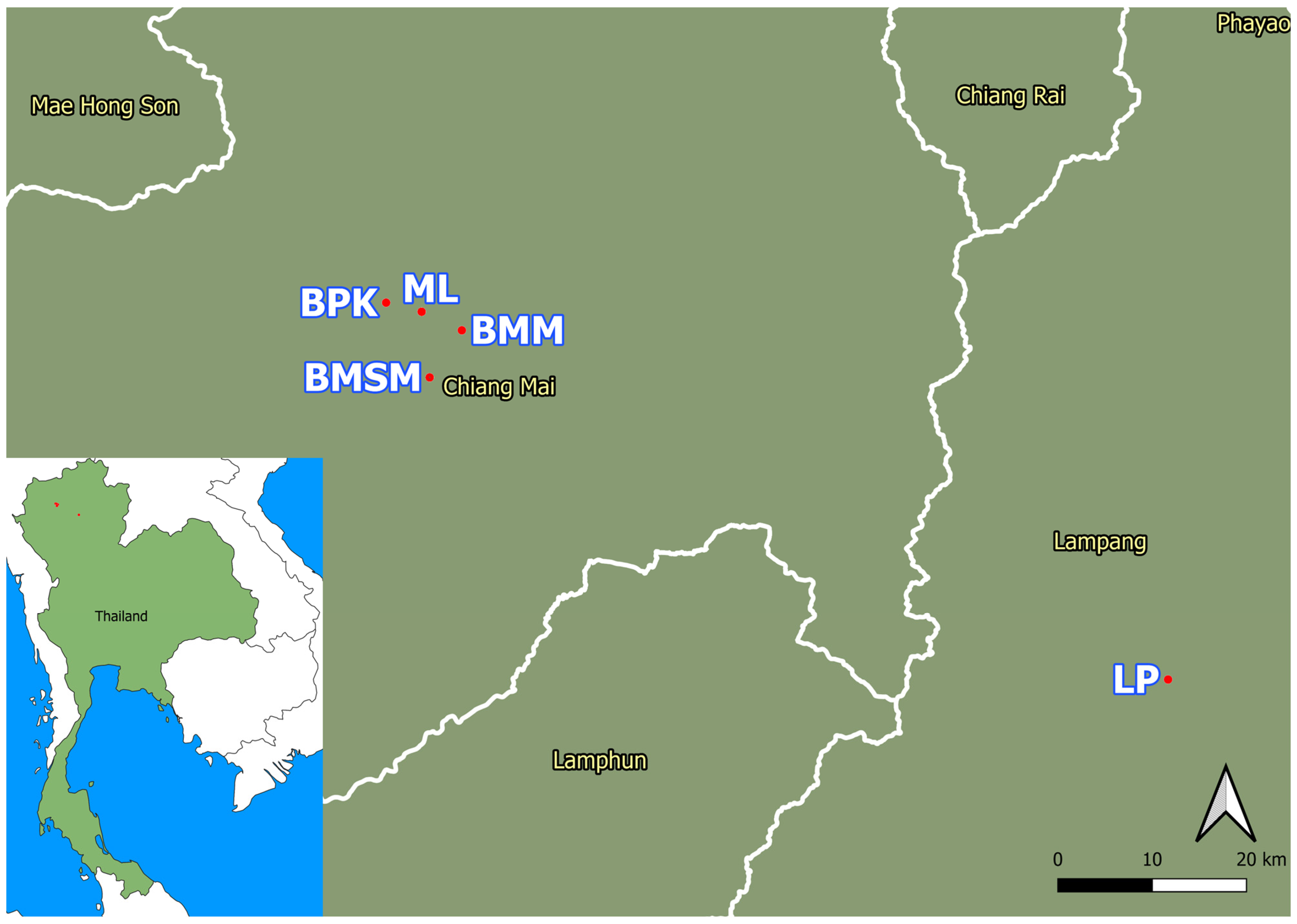
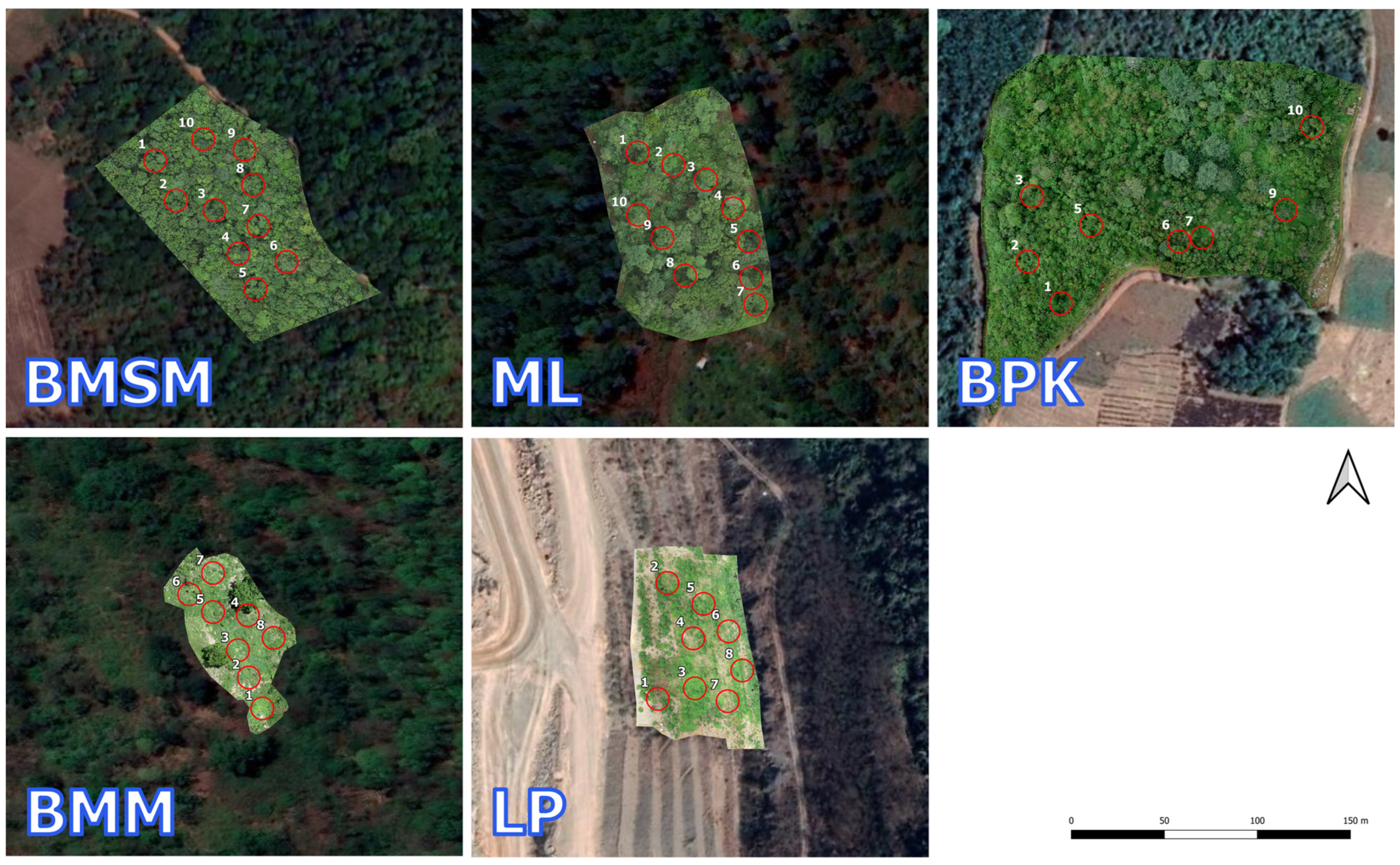
2.1. Study Sites and Equipment

Five sites, representing a range of degradation levels, were selected in the Chiang Mai and Lampang provinces, northern Thailand. Details of the sites and their acronyms are presented in Table 1, while their locations are shown in Figure 1, and orthophotos are presented in Figure 2. All sites were established by Chiang Mai University’s Forest Restoration Research Unit (FORRU-CMU) to test various forest restoration techniques. Consequently, their history was known, as were the restoration treatments that had been applied (Table 1). The sites ranged in age from 0 to 8 years since tree planting. Disturbances before restoration ranged from severe—a quarry site after mining—to abandoned agricultural sites and fire-damaged sites.
The BMSM, ML, and BPK, were all former upland evergreen forest sites, above 1200 m a.s.l. These sites were cooler and wetter (mean annual rainfall, 1736; temperatures from 4.5 °C in December to 35.5 °C in March [30]) compared to the other two sites. The BMM site, formerly mixed evergreen-deciduous forest [31], at moderate elevation (601 m a.s.l.), was drier (1119.2 mm mean annual rainfall) and warmer (11.0–41.0 °C) (data from Chiang Mai meteorological station). As was the LP site (former bamboo-deciduous forest [31]), 1196 mm mean annual rainfall, 8.2–43.0 °C temperature range (data from Lampang A meteorological station).
To compare ground data with those derived from drone imagery, circular sample plots (5 m radius) were laid out randomly across the 5 study sites: 8 or 10 plots at sites of <1 ha or >1 ha, respectively. The centre points of each plot were marked with red-black plates (Figure S1). Where tree cover obscured the centre point markers, additional markers were placed in canopy gaps, with the distance and direction to the centre-point markers being determined by a theodolite. Azimuth and distance among the points were calculated using the stadia method [32,33], such that plot centre points could be accurately placed on ortho-mosaic maps (orthophotos) derived from the drone imagery.

2.2. Data Acquisition—Ground Surveys

During ground surveys, the heights of all trees (taller than 0.5 m) in each circular sample plot were measured with an extension pole (for small trees) or laser rangefinder (for trees >8 m tall). Girth at breast height (GBH, 1.3 m above ground level) was measured using a tape measure. Tree-crown size was measured by a tape measure from below: length (longest distance) × width (perpendicular to length). In each sampling plot, percent ground cover of vegetation and exposed soil + rock was estimated by eye.

2.3. Data Acquisition—UAV Aerial Image Acquisition

Aerial surveys by drones were performed using a consumer quadcopter (DJI Phantom® 4 Pro (P4P)) (SZ DJI Technology Co., Shenzhen, China), taking RGB photographs with its on-board camera (1-inch, 20-megapixel CMOS sensor) mounted on a gimbal, which compensates for drone movement to produce sharp images. This drone is ideal for forest surveys [34] due to its relatively low cost, light weight and reasonable flight time (up to about 25 min). Object-avoidance sensors in all directions (except above) and AI-assisted landing enables safe landing and takeoff through small forest gaps.
Flight-planning software, LITCHI (https://flylitchi.com/, accessed on 5 February 2023), was used to fly the drone 50 m above ground level in a pre-programmed grid pattern over each site, with distance between grid lines (15–20 m), flight speed (10–13 m/s), and photograph frequency (3–5 s) adjusted to achieve 75%–80% overlap and sidelap between adjacent photographs and to complete each mission within the capacity of one battery (25–30 min). Details of the flight missions are provided in Table S1. Drone flights covered the entire sites, from which image data were extracted for each circular sample plot, surveyed on the ground.

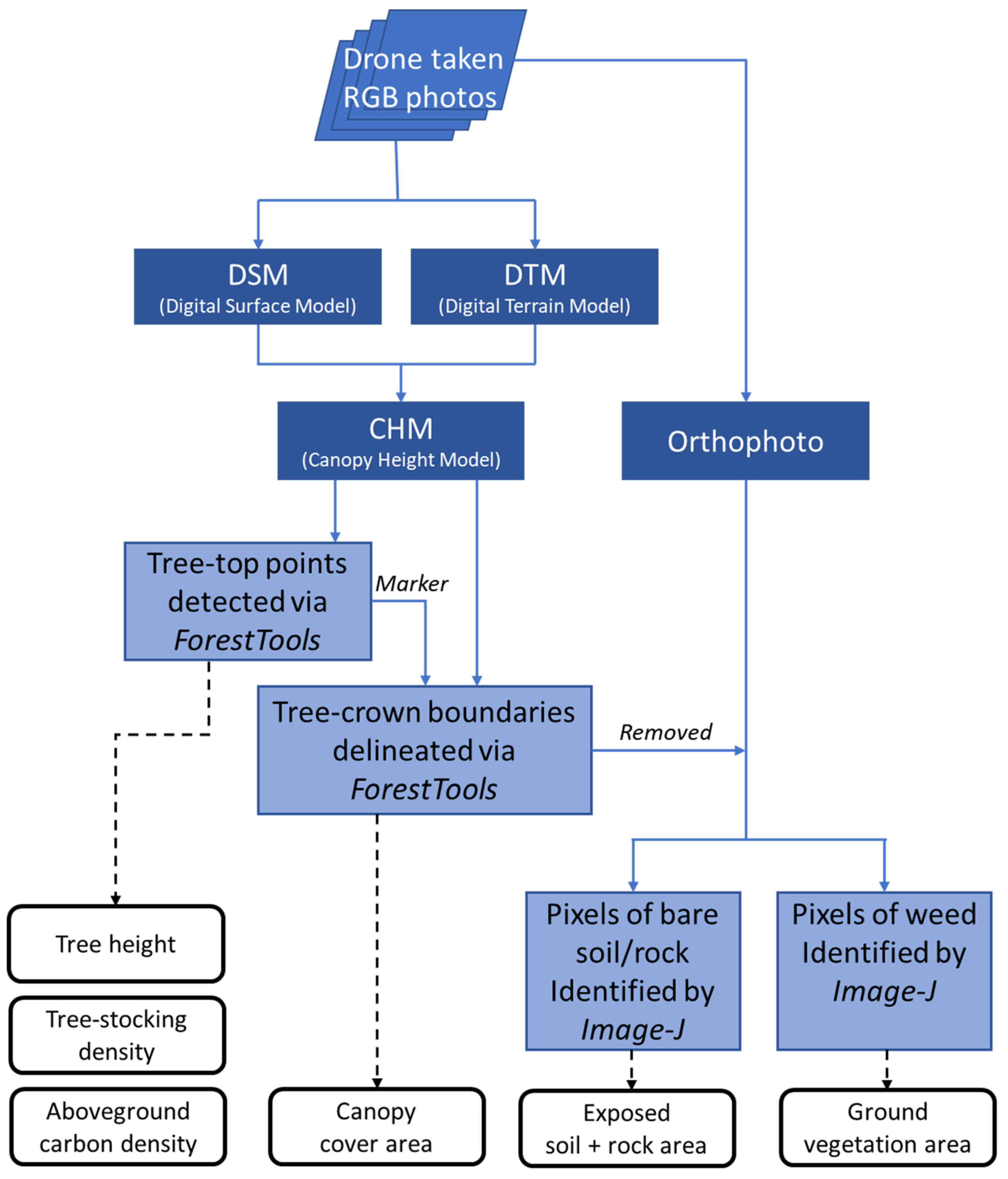
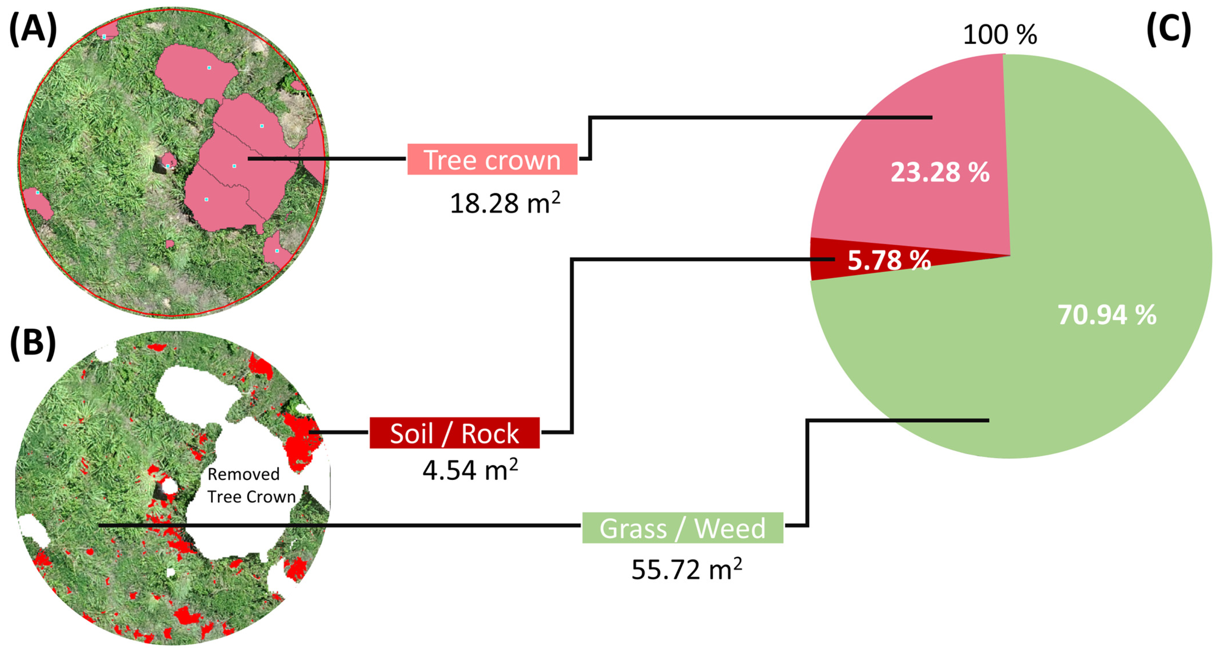
2.4. Data Processing and Analysis

Open Drone Map (ODM) (https://www.opendronemap.org/webodm/, accessed on 5 February 2023), an open source photogrammetry toolkit, hosted and distributed on GitHub, was used to process the drone imagery from each site into 3D point clouds and meshes, using an SfM algorithm. From these were generated 2D orthophotos, a digital terrain model (DTM) (representing ground topography) and a digital surface model (DSM) (representing the upper surfaces of objects). The latter two are types of digital elevation model (DEM) in raster format, with each pixel identified by its 3D coordinates. Consequently, a canopy-height model (CHM) (height above the ground) was derived by subtracting the DSM from the DTM (Figure S2). Orthophotos were compiled by aggregating overlapping images and removing radial distortion, resulting in completely vertical image maps. Between 250 and 400 pictures, generated at each site (depending on site size), were processed. DSMs and DTMs were generated at a resolution of 2 cm, and orthophotos were generated at a resolution of 1 cm—the highest precision achievable with images from the P4P camera. The texturing data term for the 3D mesh, which affects orthophoto quality, was set to “area mode”, prioritizing images covering the largest area (recommended by the tool’s developers for forest surveys). Elevation information from CHMs and colour information from orthophotos were the main variables used to assess forest degradation levels. The overall processes are described in Figure 3.

2.5. Deriving Variable Values from Collected and Processed Data

To derive stocking density (tree stems per hectare) from CHMs, tree-top points were determined using the package ‘ForestTools’ [35] (Figure S3). It works by applying a ‘variable window-filter algorithm’, which assumes that higher trees have wider crowns. The algorithm spreads circular windows, centred on each pixel sequentially of radius related to pixel height above ground. If the centre point is the highest pixel in the window, then it determines that point as a tree-top [35] (Figure S3). Tree-top points, thus detected, were counted in each plot and compared with the number of trees recorded in the ground surveys. Since small trees were obscured by the forest canopy, more were detected in ground surveys than in drone-derived photos. The number of undetected trees increased with increasing numbers of detected trees and with increasing canopy cover.
Therefore, a multiple regression model (Equation (1)), combining these two variables, was used to predict stocking density in sample plots and across the entire site (site-wide) from drone images:
t = 1.09 + 0.28 t + 0.15 c c
where  t  is the adjusted number of detected trees;  t  is number of detected trees, and  c c  is the % relative canopy cover area.
To estimate percent forest canopy cover, ground vegetation, and exposed soil + rock in drone-derived images, individual tree-crown edges were drawn on the CHMs using the ‘marker-controlled watershed segmentation (mcws)’ function in ‘ForestTools’ [35]. It delineates tree-crown boundaries by detecting the lowest height along projections radiating out from the tree-top points, where one tree-crown meets another or where the ground is detected. Minimum crown height was set at 0.5 m above the ground to prevent confusing ground vegetation with crown foliage. Detected tree-top points worked as markers of individual tree-crowns so that neighbouring or merged tree-crowns could be distinguished (Figure S4). Total canopy cover was calculated as the sum of detected tree-crown areas and expressed as a percent of sample-plot area.
From ground-based measurements of tree-crown dimensions, crown projected areas (CPA, m2) of individual trees were calculated. In each plot, all the CPAs were summed and converted to a percent of the plot area (Equation (2)). To deal with overestimation due to the overlapping crowns, we used Equation (3), as recommended by Moeur [36], Crookston and Stage [37], McIntosh et al. [38], and Adesoye and Akinwunmi [39], which relates increasing overlap with increasing total crown cover:
C = 100 i = 1 n C P A i A 1
C = 100 1 e x p 0.01 C
where  C  is the percent canopy cover without accounting for overlap.  C P A i  is crown projected area of individual trees (m2).  A  is the given area of the site (m2).  C    is the percent canopy cover accounting for overlap.
In the orthophotos, ground vegetation and tree-crowns were similar in colour. Consequently, delineated tree-crowns, derived as described above, were overlayed on the orthophotos and their pixels subtracted from the image. Remaining pixels were then classified as exposed soil or weedy vegetation using the ‘colour threshold’ tool of Image-J (https://imagej.nih.gov/ij/index.html, accessed on 5 February 2023) to vary filters for pixel hue, saturation, and brightness (HSB). Finally, all the pixels were classified as tree-canopy, ground vegetation, or exposed soil + rock. The relative cover of these three elements could then be compared between drone-derived images and ground survey estimates (Figure 4).
Max, mean, and median tree heights were measured directly in the ground surveys and derived from tree-top points, detected in the CHMs from drone-derived photos. Drone-derived above-ground carbon density (ACD) and basal area (BA) were estimated by applying Jucker et al.’s (2018) [40] regional allometric model for aerial data sets and Asian tropical forests (Equation (4)) to the mean top-of-canopy height (TCH) of each sample plot, derived from the CHM. A mean wood density value of 0.52 g/cm2 was applied, from the recent study of Pothong et al. (2021) [41] for forests in northern Thailand:
A C D MgC / ha R e g i o n a l = 0.567 × T C H 0.554 × B A 1.081 × W D 0.186
where  T C H  is the mean top-of-canopy height (m);  W D  is the local average wood density [41]; and  B A  is stand basal area (m2/ha) =  1.112 × T C H , modeled by Jucker et al. (2018) [40].
From the ground survey, above ground biomass (AGB) was calculated by applying the allometric model for northern Thailand (Equation (5)) (recently developed by destructive sampling [41]):
A G B kg = 0.134 × D 2 · H · W D 0.847
where  D  is diameter at breast height of individual tree trunks.  H  is height of individual trees.  W D  is wood density = 0.52 g/cm2, local average, studied by Pothong et al. (2021) [41].
AGB was converted to ACD using Equations (6) and (7):
A G B kg / ha = A G B kg / 78.54   m 2 ÷ 78.54   m 2 × 10,000   m 2
A C D MgC / ha = A G B kg / ha × ρ ÷ 1000   kg
where  ρ  is the local average carbon content = 0.44, Pothong et al. (2021) [41].

2.6. Statistical Analysis
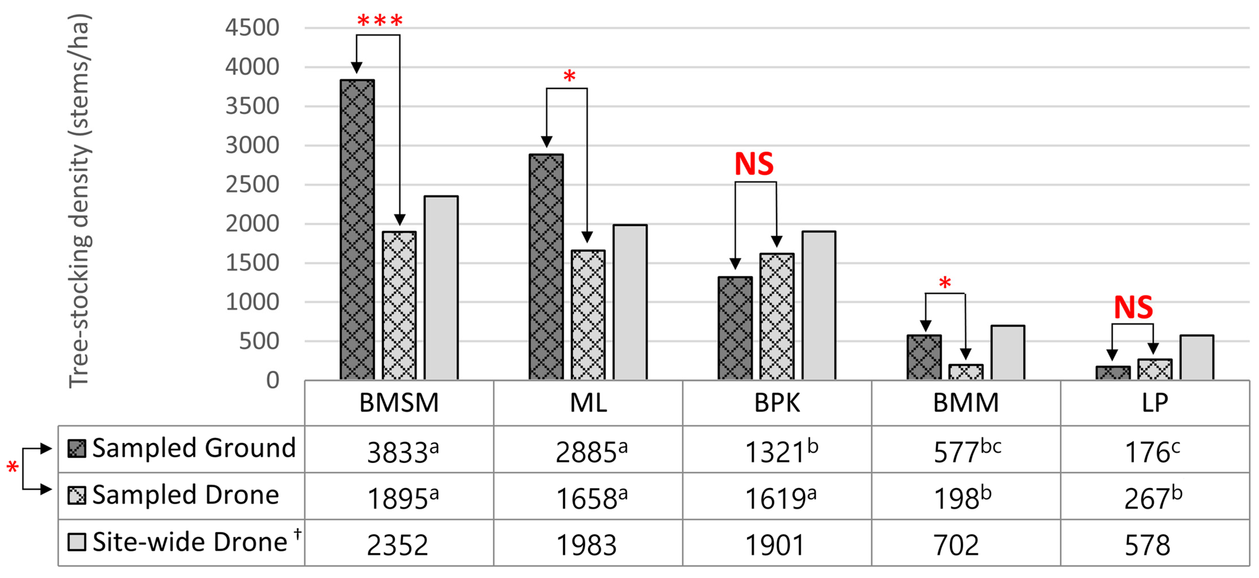
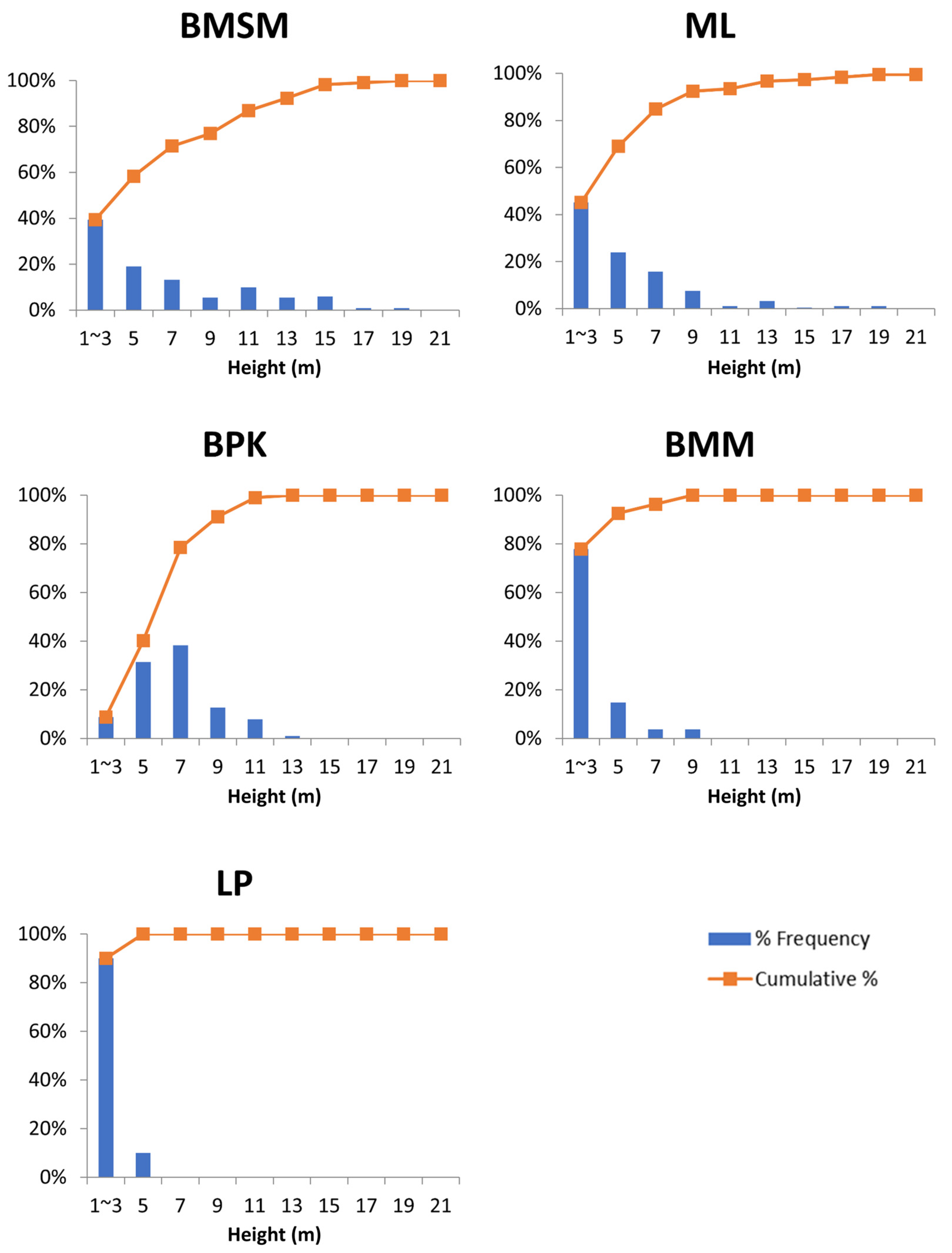
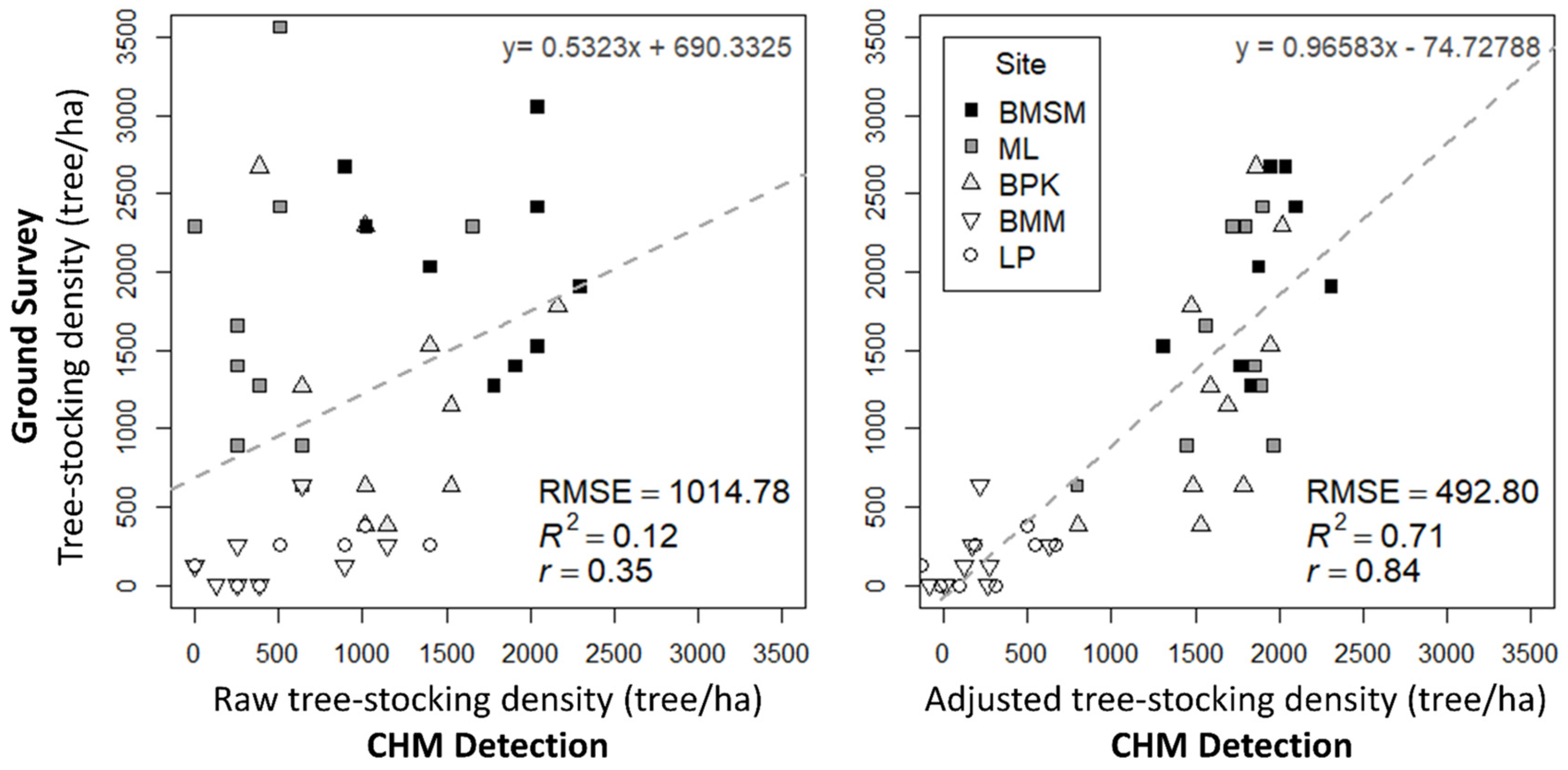
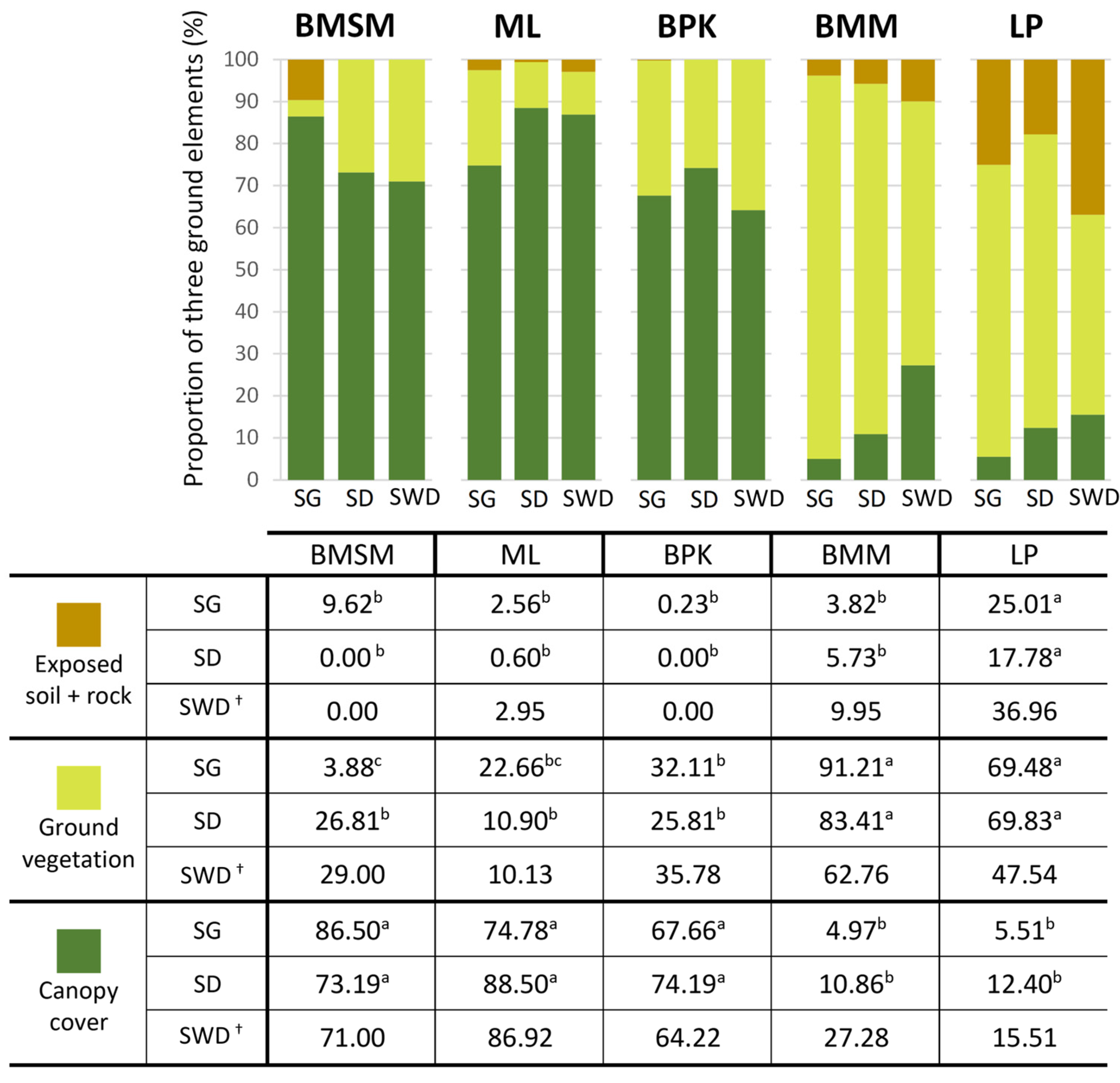
Pearson’s correlation coefficient was used to compare ground-derived with drone-derived values of each corresponding variable. Root mean square error (RMSE) was also calculated to check the size of differences between ground and aerial survey data. Significant differences in stocking density among study sites were determined to establish whether relationships between ground-derived and drone-derived data were similar across sites.
One of the disadvantages of ground-based surveys is that results for sites are extrapolated from small sample areas to estimate site-wide value, whereas drones can rapidly survey entire sites without the need for sampling and extrapolation. Consequently, sample-focused results from the drone survey were compared with directly assessed site-wide results.
Tree-size-frequency histograms were constructed for each study site to explore the influence of the proportion of small trees on tree detection in drone imagery (and hence stocking density estimates), since small trees are more likely to be obscured by taller ones when viewed from above.

3. Results

Figure 5 shows that, when estimating from sample-plot data, predictions of tree-top counts in CHMs from the multiple regression model successfully predicted measured stocking density in only 2 of the 5 sites (BPK and LP) and substantially and significantly underestimated it at the other 3 sites (by 51%, 42%, and 66%, at BMSM, ML, and BMM, respectively). Differences in percent frequency of tree size class among the sample plots from ground surveys are shown in Figure 6. A summary of ground-survey data is present in the Supplementary Materials (Table S2).
Stocking density, derived from tree-top points in the CHMs, correlated weakly with that derived from numbers of individual trees counted during ground surveys (R2 = 0.12) (Figure 7 Left). Adjusted stocking density, calculated from the model, was much more highly correlated (R2 = 0.71) with stocking density calculated from on-ground tree counts. The root mean square error (RMSE) was 493 trees per hectare, about 4 trees per 5-metre-radius plot (Figure 7 Right).
Relative cover of the three ground-cover elements (tree canopy cover, ground vegetation, and exposed soil + rock) (Figure 8) detected from drone-derived data were all highly correlated with ground-survey data. Percent canopy cover was the most highly correlated (R2 = 0.83), followed by ground vegetation (R2 = 0.71), and exposed soil + rock (R2 = 0.56) (Figure 9).
Tree height variables, derived from the CHM, were weakly correlated with the same measured in ground surveys (max, mean, and median tree height in each circular sample plot) (Figure 10). Highest correlation between drone-derived and ground data was achieved for max tree height (R2 = 0.51). Mean tree height reduced the influence of outliers, despite the weak correlation (R2 = 0.31), and was a better measure than median tree height (R2 = 0.23). Furthermore, RMSE of mean height was lower (3.3 m) than for maximum (4.1 m) and median (3.5 m) height.
CHM-derived ACD (from mean top-of-canopy height and stand basal area in each plot) was not correlated with the ACD calculated from ground-survey data (R2 = 0.24) (Figure 11 Left). When stocking density was included in the multiple regression model, correlation increased (R2 = 0.45) and RMSE was reduced (8.86 MgC/ha) (Figure 11 Right). However, overestimation of drone-derived ACD was evident in the more degraded sites: LP and BMM. Different patterns of error were found at each study site; for e.g., ACD tended to be underestimated in the BMSM plots but overestimated in the ML plots.

4. Discussion

The novelty of this research lies in the application of a cost-effective off-the-shelf drone with an RGB camera and open source software to distinguish degradation levels in trial plots of known age since the initiation of forest ecosystem restoration.
Four out of six variables derived from drone imagery were well correlated (R2 > 0.55) with the corresponding variables measured on the ground: stocking density (R2 = 0.71); relative cover of the three ground-cover elements, i.e., canopy cover (R2 = 0.83); ground vegetation (R2 = 0.71); and exposed soil + rock (R2 = 0.56). However, the other two, i.e., mean tree height (R2 = 0.31), and ACD (R2 = 0.45), were not highly correlated. These two variables were calculated from absolute height values in CHMs, whose low accuracy might be due to the absence of geo-referencing, such as ground control points (GCPs). In contrast, stocking density and percent canopy cover were well correlated, because those were derived from comparative heights in CHMs by algorithms.
One of the advantages of drone surveys is that entire sites can be surveyed rapidly. Intuitively, this should give a more accurate assessment of degradation-related variables than sampling, particularly for more severely degraded sites, where large remnant trees are distributed sparsely and can greatly skew data where they occur in sample plots. However, our study was equivocal in this respect, with inconsistent differences between the site-wide and sample-based estimates. In terms of stocking density, differences between these two estimates (Figure 5) in the less degraded sites (BMSM, ML, and BPK) were smaller (less than 25%) compared with the more degraded sites, i.e., BMM (254.6%) and LP (116.5%). The largest difference between site-wide and sample-based canopy cover estimates was at BMM (151.2%) (Figure 11), although, in contrast, the difference between the two methods at the most degraded site (LP) was small.
One of the most serious limitations of using RGB data from drone imagery is that large canopy trees obscure smaller understory trees. Furthermore, when the camera settings are correct for exposure of the sunlit upper canopy, trees in the much darker understory are substantially underexposed and can hardly be seen. Furthermore, tall ground vegetation may obscure the smallest trees, which may be detected in ground surveys but not in drone imagery.
Drone and ground tree-counts were well correlated (Figure 7). Ground and drone counts did not differ significantly at BPK and LP. However, only about half of the trees at BMSM, ML, and BMM were detectable in drone imagery. The size and nature of the differences between ground and drone tree counts (Figure 5) appeared to be site-specific.
In the least degraded sites (BMSM and ML), obscurement of the trees in drone imagery was probably due to high tree-crown cover (73.19% and 88.50%, respectively, Figure 8), caused by high representation of large trees (Figure 6). Although use of the multiple regression model (which combined the number of detected trees with canopy cover) reduced the underestimate of trees from drone imagery, it failed to fully predict the number of hidden trees. This problem may be overcome in the future by the use of lidar sensors, which are better at revealing forest understorey structure than RGB cameras [19]. However, at present, they are prohibitively expensive.
In contrast, at the more heavily degraded BMM site, where there were few trees taller than 10 m (Figure 6) to obscure smaller trees, stocking density was still underestimated by 65.69% in drone imagery. This may have been due to high weed cover; BMM supported highest weed cover for all the sites (83.41%, Figure 8). The weeds were particularly tall and dense at the BMM site. Since such a large percentage of trees were in the smallest size class (78% shorter than 2.99 m, Figure 6), it is highly likely that weeds obscured the majority of trees present in this site.
High detection of trees at BPK might be explained by the low numbers of small trees (only 9% of total trees are 1.00–2.99 m tall, Figure 6). Such a lack of small trees could be explained by the trees planted in 2016 having grown up to larger size classes and the hindrance of natural regeneration due to a lack of nearby natural forest as seed sources. Hence, most trees were in 5.00–10.99 size classes, which could be easily distinguished in drone imagery.
At LP, although the majority of trees were small, there were no large tree-crowns to obscure them (Figure 6). Weed cover was relatively sparse and not very tall. Furthermore, there were large areas of exposed mine substrate, where smaller trees showed up well against the plain grey/brown background.
GCPs are marked points on the ground, recognizable from above, whose precise coordinates are measured by GPS receivers with enhanced precision, e.g., Real-Time Kinematic (RTK) or Post-Processing Kinematic (PPK) GPS receivers. GCPs are used as thumbtacks for geo-referencing drone data, to achieve a high degree of (i) global accuracy, corresponding to the actual coordinate system and (ii) local accuracy for measurements in DEMs and orthophotos [42,43,44].
The effectiveness of geo-referencing in increasing the accuracy of canopy height, AGB, and ACD measurements was demonstrated by Zahawi et al. (2015) [25], using differential GPS, and by Swinfield et al. (2019) [28], using GCPs. Therefore, it is recommended that future studies that depend on absolute height values in CHMs should apply geo-referencing using elevation data. Specifically, the use of GCPs with precise coordinates, measured by RTK or PPK, is optimal. However, such technologies do not come as standard on off-the-shelf drones, and they are expensive. Therefore, in order to minimize errors in the positioning of sample plots in drone imagery in this study, we replaced the use of GCPs with the stadia method, which was successful at reducing locational error in sample plot positioning (Figure S5). Using 11 directly visible plots as references, the stadia method resulted in lower error in the positioning of the sample-plot centre pole (0.11–2.83, mean 0.79 m ± 0.77 SD) compared with the use of a GPS receiver (2.00–6.28 m, mean 3.71 m ± 1.45 SD). Further research is needed to compare the stadia method with the use of GCPs and to assess its practicability, since the former does require additional effort and equipment to measure the distance and direction of ground markers to sample-plot centre poles.
A barrier to the wider use of drones in forestry is high initial cost, not only of the drone itself, but also of recruiting technically proficient personnel and providing training. However, if drones are used long-term, their high initial costs are spread over many projects. Another issue is the need for complex data processing, requiring advanced software and long processing times, although the development of AI tools may reduce the time and effort needed for these tasks in the near future. Table 2 compares the relative advantages and disadvantages of using drones compared with conventional ground-based surveys. Further research is needed to quantify the relative cost-effectiveness of the two techniques.

5. Conclusions

This study aimed to explore practical and accurate solutions, using drones to replace conventional time-consuming and labour-intensive ground surveys, to help guide the implementation and monitoring of restoration projects. It focused on the development of affordable photogrammetric techniques, using RGB photography and open-source software, rather than more expensive options (e.g., lidar and hyperspectral data). While the techniques described worked well for determining stocking density and the relative proportions of ground-cover elements (forest canopy, ground vegetation, and exposed soil/rock), accurate determination of tree heights and ACD proved more difficult to achieve without GCPs. Further research is therefore needed to develop an integrated forest-degradation index that combines multiple variables derived from drone imagery as an alternative to labour-intensive and expensive ground surveys, particularly in less accessible areas.

Supplementary Materials

The following supporting information can be downloaded at: https://www.mdpi.com/article/10.3390/f14030586/s1. Figure S1: (Left) red-black ground-marker placed in the centre of circular sample plots. (Right) red-black ground marker, detected by drone image sensing; Figure S2: The canopy-height model (CHM, right) was derived by subtracting the digital terrain model (DTM, centre)) from the digital surface model (DSM, left); Figure S3: Explanation of the variable window-filter algorithm, used to detect tree-top points; Figure S4: Principle of marker-controlled watershed segmentation (mcws) algorithm, delineating crown boundaries (adopted from Fisher, 2014 [44]); Figure S5: Examples of the stadia method and comparisons with GPS-detected points in orthophotos; Table S1: Drone flight records, weather conditions, and flight-mission settings; Table S2: Summary of sampled ground dataset.

Author Contributions

Conceptualization K.L. and S.E.; methodology, K.L. and S.E.; software, K.L.; investigation, K.L. and S.E.; resources, S.E.; data analysis, K.L. and P.T.; writing—original draft preparation, K.L.; writing—review and editing, S.E. and P.T.; supervision, P.T. and S.E.; project administration, S.E.; funding acquisition, K.L. and S.E. All authors have read and agreed to the published version of the manuscript.

Funding

K.L. was fully supported by the Chiang Mai University Presidential Scholarship for the Master’s Degree Program in Environmental Science, Faculty of Science, Chiang Mai University. Research costs were partially supported by Chiang Mai University’s Forest Restoration Research Unit. The work of P.T. and S.E. on this research and manuscript was partially supported by Chiang Mai University.

Data Availability Statement

The data presented in this study are available on request from the corresponding author.

Acknowledgments

The authors thank all staff, students and interns at the FORRU-CMU, who helped with field work during this study, as well as Nophea Sasaki for reviewing this work and providing helpful comments.

Conflicts of Interest

The authors declare no conflict of interest.

References

  1. SCBD: Secretariat of the Convention on Biological Diversity. Review of the Status and Trends of, and Major Threats to, the Forest Biological Diversity (CBD Technical Series No. 7); SCBD: Montreal, QC, Canada, 2002; ISBN 92-807-2173-9. [Google Scholar]
  2. CBD. Quick Guide to the Aichi Biodiversity Targets 15. Ecosystems Restored and Resilience Enhaced; SCBD: Montreal, QC, Canada, 2010. [Google Scholar]
  3. UNFCCC. Report of the Conference of the Parties on Its Thirteenth Session, Held in Bali from 3 to 15 December 2007; UNFCCC: Bonn, Germany, 2008. [Google Scholar]
  4. Aerts, R.; Honnay, O. Forest Restoration, Biodiversity and Ecosystem Functioning. BMC Ecol. 2011, 11, 29. [Google Scholar] [CrossRef] [Green Version]
  5. Lewis, S.L.; Wheeler, C.E.; Mitchard, E.T.A.; Koch, A. Restoring Natural Forests Is the Best Way to Remove Atmospheric Carbon. Nature 2019, 568, 25–28. [Google Scholar] [CrossRef] [PubMed] [Green Version]
  6. FAO Regional Office for Asia and the Pacific. Helping Forests Take Cover On Forest Protection, Increasing Forest Cover and Future Approaches to Reforesting Degraded Tropical Landscapes in Asia and the Pacific; Poopathy, V., Appanah, S., Durst, P.B., Eds.; FAO Regional Office for Asia and the Pacific: Bangkok, Thailand, 2005; ISBN 974-7946-74-2. [Google Scholar]
  7. Zhai, D.L.; Xu, J.C.; Dai, Z.C.; Cannon, C.H.; Grumbine, R.E. Increasing Tree Cover While Losing Diverse Natural Forests in Tropical Hainan, China. Reg. Environ. Chang. 2014, 14, 611–621. [Google Scholar] [CrossRef]
  8. Höhl, M.; Ahimbisibwe, V.; Stanturf, J.A.; Elsasser, P.; Kleine, M.; Bolte, A. Forest Landscape Restoration-What Generates Failure and Success? Forests 2020, 11, 938. [Google Scholar] [CrossRef]
  9. Di Sacco, A.; Hardwick, K.A.; Blakesley, D.; Brancalion, P.H.S.; Breman, E.; Cecilio Rebola, L.; Chomba, S.; Dixon, K.; Elliott, S.; Ruyonga, G.; et al. Ten Golden Rules for Reforestation to Optimize Carbon Sequestration, Biodiversity Recovery and Livelihood Benefits. Glob. Chang. Biol. 2021, 27, 1328–1348. [Google Scholar] [CrossRef] [PubMed]
  10. Sasaki, N.; Asner, G.P.; Knorr, W.; Durst, P.B.; Priyadi, H.R.; Putz, F.E. Approaches to Classifying and Restoring Degraded Tropical Forests for the Anticipated REDD+ Climate Change Mitigation Mechanism. IForest 2011, 4, 1–6. [Google Scholar] [CrossRef] [Green Version]
  11. Elliott, S.D.; Blakesley, D.; Hardwick, K. Restoring Tropical Forests: A Practical Guide; Royal Botanic Gardens, Kew: Richmond, Surrey, UK, 2013; ISBN 978-1-84246-442-7. [Google Scholar]
  12. Thompson, I.D.; Guariguata, M.R.; Okabe, K.; Bahamondez, C.; Nasi, R.; Heymell, V.; Sabogal, C. An Operational Framework for Defining and Monitoring Forest Degradatio. Ecol. Soc. 2013, 18, 20. [Google Scholar] [CrossRef]
  13. Vásquez-Grandón, A.; Donoso, P.J.; Gerding, V. Forest Degradation: When Is a Forest Degraded? Forests 2018, 9, 726. [Google Scholar] [CrossRef] [Green Version]
  14. Alonzo, M.; Andersen, H.E.; Morton, D.C.; Cook, B.D. Quantifying Boreal Forest Structure and Composition Using UAV Structure from Motion. Forests 2018, 9, 119. [Google Scholar] [CrossRef] [Green Version]
  15. Camarretta, N.; Harrison, P.A.; Bailey, T.; Potts, B.; Lucieer, A.; Davidson, N.; Hunt, M. Monitoring Forest Structure to Guide Adaptive Management of Forest Restoration: A Review of Remote Sensing Approaches. New For. 2019, 51, 573–596. [Google Scholar] [CrossRef]
  16. Asner, G.P.; Martin, R.E.; Anderson, C.B.; Knapp, D.E. Quantifying Forest Canopy Traits: Imaging Spectroscopy versus Field Survey. Remote Sens. Environ. 2015, 158, 15–27. [Google Scholar] [CrossRef]
  17. Paneque-Gálvez, J.; McCall, M.K.; Napoletano, B.M.; Wich, S.A.; Koh, L.P. Small Drones for Community-Based Forest Monitoring: An Assessment of Their Feasibility and Potential in Tropical Areas. Forests 2014, 5, 1481–1507. [Google Scholar] [CrossRef] [Green Version]
  18. Sankey, T.; Donager, J.; McVay, J.; Sankey, J.B. UAV Lidar and Hyperspectral Fusion for Forest Monitoring in the Southwestern USA. Remote Sens. Environ. 2017, 195, 30–43. [Google Scholar] [CrossRef]
  19. de Almeida, D.R.A.; Broadbent, E.N.; Ferreira, M.P.; Meli, P.; Zambrano, A.M.A.; Gorgens, E.B.; Resende, A.F.; de Almeida, C.T.; do Amaral, C.H.; Corte, A.P.D.; et al. Monitoring Restored Tropical Forest Diversity and Structure through UAV-Borne Hyperspectral and Lidar Fusion. Remote Sens. Environ. 2021, 264, 112582. [Google Scholar] [CrossRef]
  20. Asner, G.P.; Mascaro, J.; Muller-Landau, H.C.; Vieilledent, G.; Vaudry, R.; Rasamoelina, M.; Hall, J.S.; van Breugel, M. A Universal Airborne LiDAR Approach for Tropical Forest Carbon Mapping. Oecologia 2012, 168, 1147–1160. [Google Scholar] [CrossRef] [PubMed]
  21. Wallace, L.; Lucieer, A.; Malenovskỳ, Z.; Turner, D.; Vopěnka, P. Assessment of Forest Structure Using Two UAV Techniques: A Comparison of Airborne Laser Scanning and Structure from Motion (SfM) Point Clouds. Forests 2016, 7, 62. [Google Scholar] [CrossRef] [Green Version]
  22. Ullman, S. The Interpretation of Structure From Motion. R. Soc. Lond. 1979, 203, 405–426. [Google Scholar] [CrossRef] [Green Version]
  23. Stockman, G.; Shapiro, L.G. Computer Vision; Prentice Hall: Hoboken, NJ, USA, 2001; ISBN 978-0-13-030796-5. [Google Scholar]
  24. Zahawi, R.A.; Dandois, J.P.; Holl, K.D.; Nadwodny, D.; Reid, J.L.; Ellis, E.C. Using Lightweight Unmanned Aerial Vehicles to Monitor Tropical Forest Recovery. Biol. Conserv. 2015, 186, 287–295. [Google Scholar] [CrossRef] [Green Version]
  25. Fujimoto, A.; Haga, C.; Matsui, T.; Machimura, T.; Hayashi, K.; Sugita, S.; Takagi, H. An End to End Process Development for UAV-SfM Based Forest Monitoring: Individual Tree Detection, Species Classification and Carbon Dynamics Simulation. Forests 2019, 10, 680. [Google Scholar] [CrossRef] [Green Version]
  26. Khokthong, W.; Zemp, D.C.; Irawan, B.; Sundawati, L.; Kreft, H.; Hölscher, D. Drone-Based Assessment of Canopy Cover for Analyzing Tree Mortality in an Oil Palm Agroforest. Front. For. Glob. Chang. 2019, 2, 12. [Google Scholar] [CrossRef] [Green Version]
  27. Swinfield, T.; Lindsell, J.A.; Williams, J.V.; Harrison, R.D.; Agustiono; Habibi; Elva, G.; Schönlieb, C.B.; Coomes, D.A. Accurate Measurement of Tropical Forest Canopy Heights and Aboveground Carbon Using Structure From Motion. Remote Sens. 2019, 11, 928. [Google Scholar] [CrossRef] [Green Version]
  28. Zhou, X.; Zhang, X. Individual Tree Parameters Estimation for Plantation Forests Based on UAV Oblique Photography. IEEE Access 2020, 8, 96184–96198. [Google Scholar] [CrossRef]
  29. Glomvinya, S.; Tantasirin, C.; Tongdeenok, P.; Tanaka, N. Changes in Rainfall Characteristics at Huai Kog-Ma Watershed, Chiang Mai Province. Thai J. For. 2016, 35, 66–77. [Google Scholar]
  30. Maxwell, J.F.; Elliott, S. Vegetation and Vascular Flora of Doi Sutep-Pui National Park, Chiang Mai Province, Thailand; Biodiversity Research and Training Program: Bangkok, Thailand, 2001; ISBN 947-7360-61-6. [Google Scholar]
  31. Benton, A.R.T.; Taetz, P.J. Elements of Plane Surveying; McGraw-Hill Inter: London, UK, 1991; ISBN 978-0070048843. [Google Scholar]
  32. Brinker, R.C.; Wolf, P.R. Elementary Surveying, 7th ed.; Harper & Row: New York, NY, USA, 1984; ISBN 978-0060409821. [Google Scholar]
  33. Brach, M.; Chan, J.C.W.; Szymański, P. Accuracy Assessment of Different Photogrammetric Software for Processing Data from Low-Cost UAV Platforms in Forest Conditions. IForest 2019, 12, 435–441. [Google Scholar] [CrossRef] [Green Version]
  34. Plowright, A.; Roussel, J.-R. ForestTools: Analyzing Remotely Sensed Forest Data; R Package Version 0.2.1; 2020. [Google Scholar]
  35. Moeur, M. Predicting Canopy Cover and Shrub Cover with the Prognosis-COVER Model. In Wildlife: Modeling Habitat Relationships of Terrestrial Vertebrates; Verner, J., Morrison, M., Ralph, L., John, C., Eds.; The University of Wisconsin Press: Madison, WI, USA, 1986; p. 470. [Google Scholar]
  36. Crookston, N.L.; Stage, A.R. Percent Canopy Cover and Stand Structure Statistics from the Forest Vegetation Simulator; U.S. Department of Agriculture, Forest Service, Rocky Mountain Research Station: Ogden, UT, USA, 1999.
  37. McIntosh, A.C.S.; Gray, A.N.; Garman, S.L. Estimating Canopy Cover from Standard Forest Inventory Measurements in Western Oregon. For. Sci. 2012, 58, 154–167. [Google Scholar] [CrossRef] [Green Version]
  38. Adesoye, P.; Akinwunmi, A.A. Tree Slenderness Coefficient and Percent Canopy Cover in Oban Group Forest, Nigeria Tree Slenderness Coefficient and Percent Canopy Cover in Oban. J. Nat. Sci. Res. 2016, 6, 9–17. [Google Scholar]
  39. Jucker, T.; Asner, G.P.; Dalponte, M.; Brodrick, P.G.; Philipson, C.D.; Vaughn, N.R.; Arn Teh, Y.; Brelsford, C.; Burslem, D.F.R.P.; Deere, N.J.; et al. Estimating Aboveground Carbon Density and Its Uncertainty in Borneo’s Structurally Complex Tropical Forests Using Airborne Laser Scanning. Biogeosciences 2018, 15, 3811–3830. [Google Scholar] [CrossRef]
  40. Pothong, T.; Elliott, S.; Chairuangsri, S.; Chanthorn, W.; Shannon, D.P.; Wangpakapattanawong, P. New Allometric Equations for Quantifying Tree Biomass and Carbon Sequestration in Seasonally Dry Secondary Forest in Northern Thailand. New For. 2021, 53, 17–36. [Google Scholar] [CrossRef]
  41. Coveney, S.; Roberts, K. Lightweight UAV Digital Elevation Models and Orthoimagery for Environmental Applications: Data Accuracy Evaluation and Potential for River Flood Risk Modelling. Int. J. Remote Sens. 2017, 38, 3159–3180. [Google Scholar] [CrossRef] [Green Version]
  42. DroneDeploy When To Use Ground Control Points: How To Decide If Your Drone Mapping Project Needs GCPs. Available online: https://medium.com/aerial-acuity/when-to-use-ground-control-points-2d404d9f5b15 (accessed on 5 February 2023).
  43. Sanz-Ablanedo, E.; Chandler, J.H.; Rodríguez-Pérez, J.R.; Ordóñez, C. Accuracy of Unmanned Aerial Vehicle (UAV) and SfM Photogrammetry Survey as a Function of the Number and Location of Ground Control Points Used. Remote Sens. 2018, 10, 1606. [Google Scholar] [CrossRef] [Green Version]
  44. Fisher, A. Cloud and Cloud-Shadow Detection in SPOT5 HRG Imagery with Automated Morphological Feature Extraction. Remote Sens. 2014, 6, 776–800. [Google Scholar] [CrossRef] [Green Version]
Figure 1. Location of the 5 study sites in the Chiang Mai and Lampang provinces, northern Thailand. White lines are province boundaries within Thailand.
Forests 14 00586 g001
Figure 2. Orthophotos showing the size, shape, and boundaries of the five sites with a unified scale: BMSM = Ban Mae Sa Mai, ML = Mon Long, BPK = Ban Pong Krai, BMM = Ban Meh Meh and LP = Lampang. Red circles are sample plots. White figures are plot id. numbers.
Forests 14 00586 g002
Figure 3. Flowchart of processing the drone RGB imagery to quantify indicator variables.
Forests 14 00586 g003
Figure 4. Example of separating three ground-cover elements: (A) Canopy cover, merged tree-crown boundaries, delineated from CHM. (B) Canopy cover pre-removed orthophoto, exposed soil + rock detection using colour threshold. (C) Percent three ground elements. CHM = Canopy-height model.
Forests 14 00586 g004
Figure 5. A comparison of mean stocking density estimates at Ban Mae Sa Mai (BMSM), Mon Long (ML), Ban Pong Krai (BPK), Ban Meh Meh (BMM), and the Lampang quarry (LP), among ground- and drone-based surveys of sample plots only (SG and SD, respectively) and site-wide drone-based assessments (drone estimates from the multiple regression model). Drones estimates from the mean values within rows, not sharing the same superscript, are significantly different (p < 0.05). Site-wide estimates are absolute values (hence no superscripts). Asterisks indicate a significant difference between two methods: * (p < 0.05); *** (p < 0.001). NS = non-significant.
Forests 14 00586 g005
Figure 6. Percent frequency of tree size classes from ground surveys in sample plots for each site. (BMSM): Ban Mae Sa Mai; (ML): Mon Long; (BPK): Ban Pong Krai; (BMM): Ban Meh Me; (LP): Lampang.
Forests 14 00586 g006
Figure 7. Stocking density (stems/ha), extrapolated from circular sample plots (5 m radius) from ground-based tree counts vs. drone imagery (tree-top counts from crown height models (left) and a multiple regression model combining tree-top counts and canopy density (right). RMSE = root mean square error; r = Pearson’s correlation coefficient. Each point represents one circular sample plot. Sites are indicated by the shape and shading of the points.
Forests 14 00586 g007
Figure 8. Percent of three ground-cover elements averaged from sample plots. (BMSM): Ban Mae Sa Mai; (ML): Mon Long; (BPK): Ban Pong Krai; (BMM): Ban Meh Me; (LP): Lampang. (SG): Sampled ground survey; (SD) Sampled drone survey; (SWD) Site-wide drone survey of each whole site. a–c within each row, comparing sites, means without a common superscript significantly differ (p < 0.05); Absence of significance symbols for SWD, as these are not mean values but absolute values.
Forests 14 00586 g008
Figure 9. Scatter plots of the percent of three ground-elements. (Left) Percent canopy cover. (Right) Percent ground vegetation. (Lower) Percent exposed soil + rock. (CHM): Canopy-height model; (RMSE): Root mean square error; (r): Pearson’s correlation coefficient.
Forests 14 00586 g009
Figure 10. Scatter plots of tree height variables: (Left) Max height. (Right) Mean height. (Lower) Median height. CHM = Canopy-height model; RMSE = Root mean square error; r = Pearson’s correlation coefficient.
Forests 14 00586 g010
Figure 11. Scatter plots of ACD: (Left) ACD from CHM. (Right) Adjusted ACD from a multiple regression model, with ACD and stocking density from CHM. ACD = Above-ground carbon density; CHM = Canopy-height model; RMSE = Root mean square error; r = Pearson’s correlation coefficient.
Forests 14 00586 g011
Table 1. Details of the 5 study sites in northern Thailand.
SiteRestoration InitiatedSite HistoryLongitudeLatitudeAltitude
(m a.s.l.)
Area,
No. Circular
Sample Plots
Ban Mae Sa Mai2012Upland evergreen forest, cleared for agriculture, abandoned in the 1990′s, invaded by herbaceous weeds, and subsequently burnt multiple times; planted with framework tree species in 2007; burnt in 2010 and replanted in 201298°50′57″18°51′22″1247 m1.07 ha
10 plots
Mon Long2014Upland evergreen forest, impacted by fire; enrichment planting with framework tree species amongst scattered remnant mature trees in 201498°50′28″18°55′20″1290 m1.03 ha
10 plots
Ban Pong Krai2016Upland evergreen forest cleared for agriculture undergoing natural regeneration; planted with framework tree species in 201698°48′19″18°55′52″1408 m2.69 ha
10 plots
Ban Meh Meh2020Mixed evergreen-deciduous forest cleared for agriculture and used for domestic elephant browsing; some natural regeneration from surrounding remnant forest, complemented with planting framework tree species in 202098°52′53″18°54′13″601 m0.41 ha
8 plots
Lampang2019Limestone quarry floor; vegetation and top soil removed; benches (terraces) planted with native forest tree seedlings 1 year previously99°35′23″18°33′12″419 m0.66 ha
8 plots
Table 2. Comparison between ground and drone survey methods.
Cost TypeGround SurveyDrone Survey
SetupTraining
Relatively simple techniques
Short training period
Steep learning curve
Longer training period
Equipment
Cheaper
More expensive
Data
acquisition
(Field)
Time
More time consuming
Rapid data collection
Labour
(Salary, food)
3–4 teams × 2–4 members
More expense
1 team × 3 members
Less expense
Weather
limitations
Limited only by severe weather that may affect worker safety
Highly sensitive to minor weather changes, e.g., poor lighting conditions, low clouds, mist, light rain, wind, etc.
Data
processing
(Lab)
Technique
Simple spreadsheet software—free or relatively cheap
Low power computers adequate
Advanced software required with costly licenses
Powerful computers needed
Disclaimer/Publisher’s Note: The statements, opinions and data contained in all publications are solely those of the individual author(s) and contributor(s) and not of MDPI and/or the editor(s). MDPI and/or the editor(s) disclaim responsibility for any injury to people or property resulting from any ideas, methods, instructions or products referred to in the content.

