Classification of Individual Tree Species Using UAV LiDAR Based on Transformer

Abstract

Tree species surveys are crucial in forest resource management and can provide references for forest protection policymakers. Traditional tree species surveys in the field are labor-intensive and time-consuming. In contrast, airborne LiDAR technology is highly capable of penetrating forest vegetation; it can be used to quickly obtain three-dimensional information regarding vegetation over large areas with a high level of precision, and it is widely used in the field of forestry. At this stage, most studies related to individual tree species classification focus on traditional machine learning, which often requires the combination of external information such as hyperspectral cameras and has difficulty in selecting features manually. In our research, we directly processed the point cloud from a UAV LiDAR system without the need to voxelize or grid the point cloud. Considering that relationships between disorder points can be effectively extracted using Transformer, we explored the potential of a 3D deep learning algorithm based on Transformer in the field of individual tree species classification. We used the UAV LiDAR data obtained in the experimental forest farm of Northeast Forestry University as the research object, and first, the data were preprocessed by being denoised and ground filtered. We used an improved random walk algorithm for individual tree segmentation and made our own data sets. Six different 3D deep learning neural networks and random forest algorithms were trained and tested to classify the point clouds of three tree species. The results show that the overall classification accuracy of PCT based on Transformer reached up to 88.3%, the kappa coefficient reached up to 0.82, and the optimal point density was 4096, which was slightly higher than that of the other deep learning algorithms we analyzed. In contrast, the overall accuracy of the random forest algorithm was only 63.3%. These results show that compared with the commonly used machine learning algorithms and a few algorithms based on multi-layer perceptron, Transformer-based networks provide higher accuracy, which means they can provide a theoretical basis and technical support for future research in the field of forest resource supervision based on UAV remote sensing.

1. Introduction

Forests are the main natural resources on Earth and play an indispensable role in the process of environmental self-regulation, such as the energy exchange between the land surface and atmosphere [1]. Forest resources mapping is mainly carried out using remote sensing data, and tree species classification is an important part of forest resources mapping [2,3]. With the rapid development of modern science and technology, traditional forest survey methods, which consume a large amount of manpower and financial resources, are gradually being replaced by emerging remote sensing technology [4]. Precision forestry has become a trend in the development of the forestry industry. New survey methods such as satellite remote sensing, laser radar (LiDAR, light detection and ranging), and unmanned aerial vehicle remote sensing have gradually come to represent typical directions of research. LiDAR technology is an active remote sensing technology. Its laser pulse demonstrates good penetrability in forests, and the high sampling density it offers means it can be used to obtain the three-dimensional structural characteristics of a single tree [5], which are widely used in forestry research. According to different data acquisition platforms, LiDAR technology can be divided into three categories: ground-based [6], airborne [7], and spaceborne [8]. Spaceborne LiDAR technology acquires a large amount of information and has a long acquisition period with low relative accuracy, which means it is only applicable to large-scale and long-period forestry surveys. Compared with airborne LiDAR data, UAV (unmanned aerial vehicle) LiDAR data have lower associated costs and higher point cloud density, which are obviously advantageous traits in the field of forest information acquisition. Brandtberg’s research [9] on deciduous forests in Virginia proved that LiDAR data can be used to classify certain deciduous trees earlier.

There are two main steps to complete the tree species classification pipeline. One is automatic individual tree segmentation and the other is tree species classification, which our research focuses on in this research. Some scholars have achieved similar research goals by using machine learning. Cao et al. [10] used full waveform LiDAR data to identify single tree species in subtropical forests. Their results showed that the overall classification accuracy of six types of trees was 68.6%, four types of trees was 75.8%, and coniferous forests and broad-leaved forests was 86.2%. Based on the airborne LiDAR data, Li et al. [11] classified four species of coniferous and broad-leaved forests with an overall accuracy of 77.5% by extracting the three-dimensional texture, clustering degree, and tree gap information related to trees and by using a genetic algorithm to select features. Kim et al. [12] separated the information related to a single tree based on multi-temporal airborne LiDAR data and classified and identified it according to the echo intensity of the trees before and after defoliation. The results showed that the joint recognition of the data before and after defoliation was the best, with an accuracy of 90.6%. Shoot et al. [13] used a combination of airborne hyperspectral and LiDAR data, showing that the random forest classification algorithm with the hyperspectral vegetation index and LiDAR-derived terrain and canopy height indicators had the highest level of accuracy (the overall accuracy was 78%).

Most studies above regarding individual tree species classification are based on traditional machine learning algorithms such as random forests or support vector machines. And some studies [14] used multi-source remote sensing data such as LiDAR and hyperspectral data. The data used in these studies are associated with large data redundancy and difficulty in the manual selection of features. With the sustainable development of graphics hardware, especially the performance of parallel computing, deep learning technology has been developed in terms of processing 3D data. Compared with machine learning, deep learning is more effective when used for feature extraction. Gradually, scholars began to study the application of deep learning in tree point cloud classification and recognition. Sun et al. [15] transformed LiDAR data into a canopy height model (CHM) and classified it with a modified convolutional neural network after segmentation. Mizoguchi et al. [16] converted 3D point clouds into images to facilitate classification tasks based on the bark surfaces of two species, and it was shown that their classification accuracy was usually greater than 90%. In these studies, the point cloud was usually converted to other formats first, but this technique generally means that some information is lost [17]. In recent years, some scholars have also used 3D deep learning in this field. For example, Liu et al. [18] used the method which proposed the use of the LayerNet network, based on multi-layer perceptron (MLP), to classify the point clouds of two species of trees from UAV laser scanning and TLS (terrestrial laser scanning), and a high level of accuracy was obtained.

In the field of point cloud classification tasks using deep learning algorithms, common structures are based on multi-layer perceptron, such as PointNet and PointNet++ [19,20]. These approaches overcome the difficulty of convolution in computing, but it is difficult to consider the relationship between points. Another concept applied to the deep learning of point clouds is to design an operator with permutation invariance which is independent of the connection relationship of European spatial points to deal with point clouds. The core part of the Transformer [21] structure proposed by the Google team in 2017 is the attention mechanism, which is always used as an auxiliary module to enhance the ability of the model to extract important features in some convolution networks to improve the integer effect. The attention mechanism itself is an operator that does not change the arrangement and does not rely on the connection between points. Its self-attention mechanism follows simple setting operations. It is not affected by the cardinality and arrangement of input features. It can easily understand the relationship between sparse point clouds in 3D scenes and is suitable for use in processing point cloud data. In recent years, an increasing number of scholars have applied Transformer in point cloud tasks, such as Point-MAE in point cloud classification tasks [22]. Considering the number of classes and the difficulty of pre-training, our research attempted to use a deep learning algorithm called PCT (point cloud transformer) proposed by Guo et al. [23] in this study. The individual tree segmentation results were made and sent into the classifier after processing for the corresponding training and testing sets, so as to achieve the classification of Quercus mongolica (the Latin name is Quercus mongolica Fisch.ex Ledeb.), birch (the Latin name is Betula platyphylla Suk.), and sylvestris (the Latin name is Pinus sylvestris var.mongholica Litv.); Classification of individual tree species was completed and the potential of the emerging deep learning algorithm framework was explored based on Transformer in this field.

2. Materials and Methods

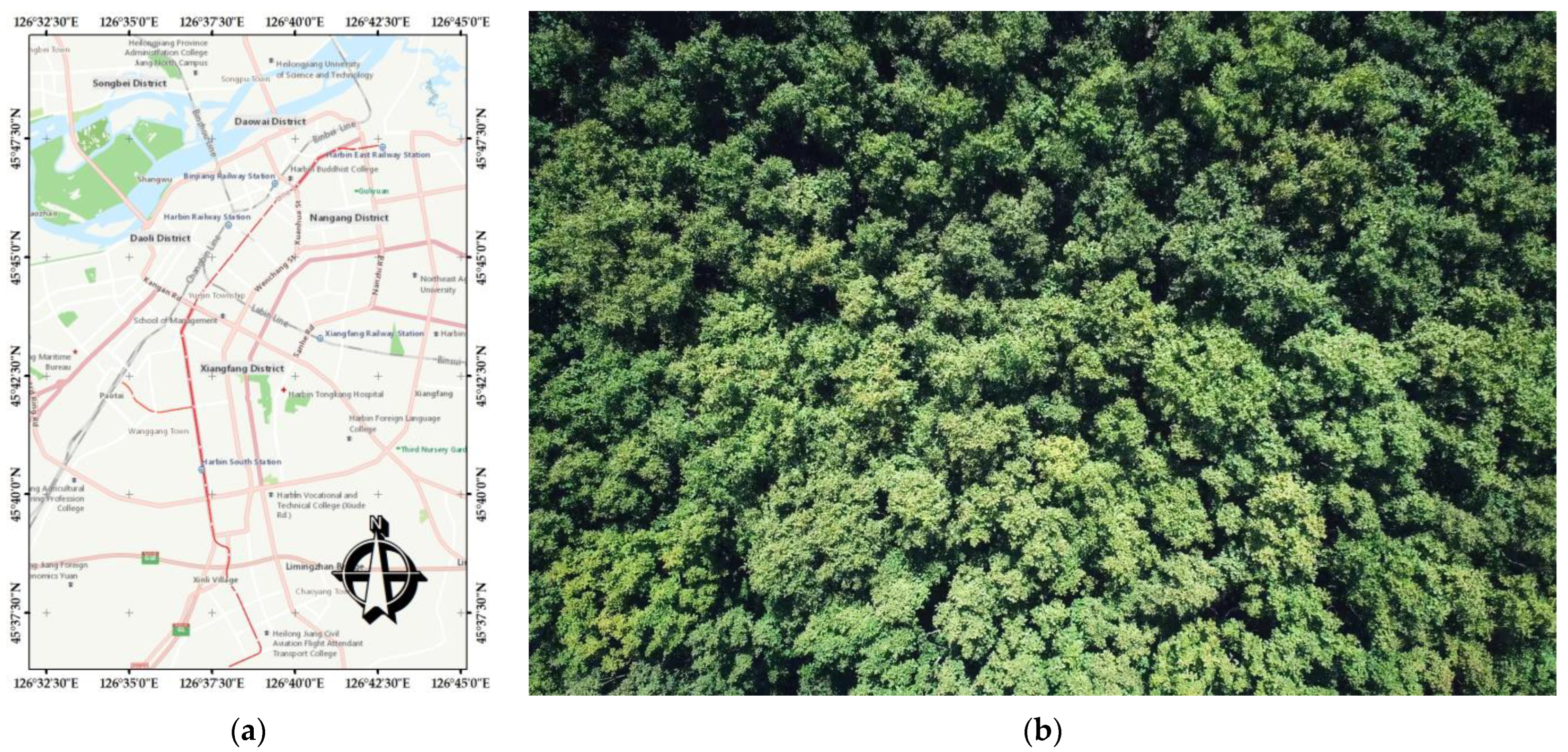
2.1. Study Area

The study area shown in Figure 1 is the urban forestry demonstration base of Northeast Forestry University (126°63′15″ E, 45°43′ N), which is located at the junction of NanGang District and XiangFang District, Harbin, Heilongjiang Province, and adjacent to Majiagou River, covering an area of 43.95 ha. With an altitude of 136~140 m, the original vegetation is valley elm, sparse forest, and grassland. There are 46 sample plots and 18 kinds of artificial forests in the forest farm, which is a large “forest oxygen bar” in Harbin. The study area has a temperate, continental, monsoon climate, with mild and rainy summers and cold and dry winters. The main tree species are Larix gmelinii and Fraxinus mandshurica. The mixed forest type is broad-leaved mixed forests and coniferous mixed forests, which provided a basis for the identification of tree species.

2.2. Data Acquisition

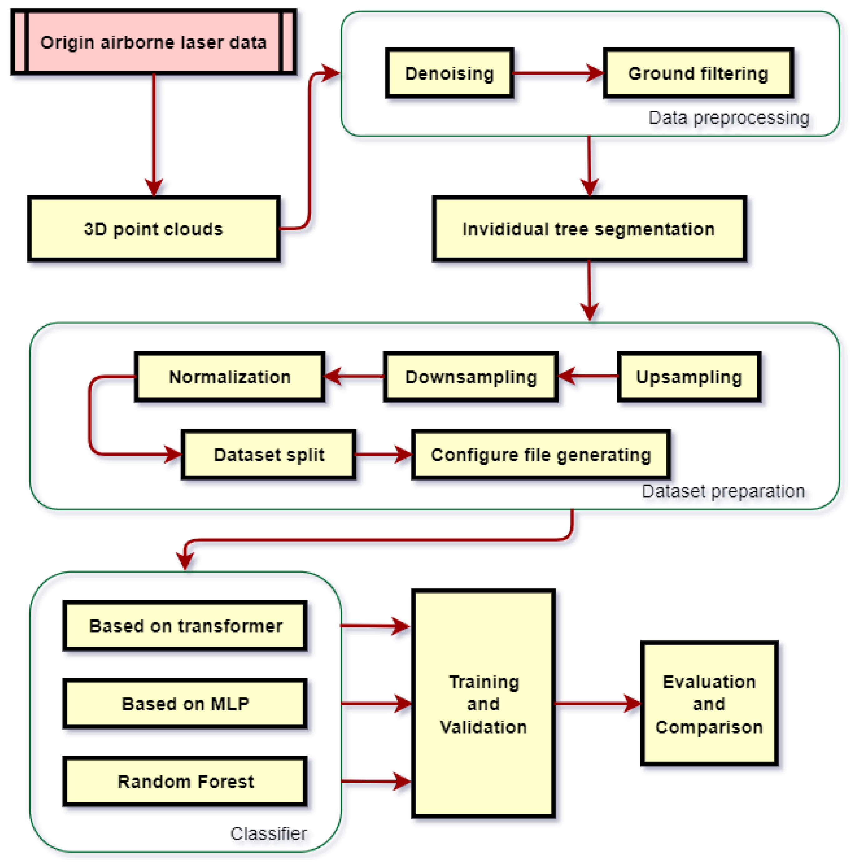
The LiDAR data used in the experiment was obtained using a Zenmuse L1 laser radar carried by DJI MTK R300. A continuous rectangle area containing three tree species was selected as the data collection site. The scanning took place on September 2, 2022 and took approximately 40 min. Normal flight was adopted, and the route height was set to 35 m. The vehicle speed was 3 m/s, and the laser side overlap rate was 65% to achieve maximum efficiency during data acquisition. The sample rate was 160 khz, and the three-echo mode was adopted. The scanning mode was repeated. The point cloud density was 1772 points/m². The original data obtained were a set of files, including laser data, RTK data, camera calibration data, etc. The standard format file of LiDAR (.LAS) can be obtained through the reconstruction of DJI Terra. To facilitate subsequent processing, the point cloud files were converted to the standard format of the point cloud database. Figure 2 shows the point cloud file obtained by scanning the study area using ULS (unmanned aerial vehicle laser scanning). The details of the parameters are shown in

Table 1. ULS parameter settings.

Instrument Parameters	Zenmuse L1 Settings
Flying height	35 m
Flying speed	3 m/s
Point cloud density	1772 points/m2
Side overlap	65%
Course angle	28°
Echo mode	Triple
Sample rate	160 khz
Scan mode	Repeat

.

2.3. Methodology

The methodological workflow (Figure 3) consisted of the following steps: (1) preprocessing to gain a simplified forest point cloud, including denoising and ground filtering; (2) individual tree segmentation to obtain a single tree point cloud; (3) creating our own data set, resampling, normalizing, and centralizing the single tree point cloud, adding labels and then dividing the training set and test set; (4) classifier selection, including training and parameter adjustment; and (5) comparative experiments and evaluation, and the comparison of the performance of several deep learning and machine learning algorithms in this task.

2.3.1. Preprocessing

Data preprocessing included the following steps, which mainly comprised denoising and ground filtering. The following operations were mostly completed by using the open-source software CloudCompare and combining the PCL library and Python in the Linux environment:

• Denoising

When obtaining point cloud data, due to the accuracy of the equipment, the surrounding environment, and other factors, some noise will inevitably appear in the point cloud data, which may lead to deviation in the results. Firstly, the KNN algorithm was used for noise reduction. The K value was set to 12 and the threshold value was set to 1.2 so as to distinguish between noisy and non-noisy points. Then, points larger than this threshold value were eliminated through calculation, and the point number of point clouds processed was reduced from $2.26\times {10}^7$ to $1.76\times {10}^7$. The comparison between the original data and the denoised data is shown in Figure 4.

2.

Ground filtering

In order to carry out subsequent experiments more effectively, the ground points are needed to separate. Therefore, the cloth filtering (CSF) algorithm proposed by Zhang et al. [24] is selected. In traditional filtering algorithms, the difference between slope and elevation changes are mostly considered to distinguish ground points from non-ground points. They are not only vulnerable to the impact of terrain features (usually poor filtering effects in complex scenes and steep terrain areas), but also often require users to have rich prior knowledge of the data to set various parameters in the filter. In the cloth filtering algorithm, a completely new concept is used to filter data. First, the point cloud is inverted, and then, it is assumed that a piece of cloth falls from above under gravity so that the fallen cloth can represent the current terrain. Here, the resolution of the cloth mesh is set to 0.2, the maximum number of iterations is set to 500, and the threshold value is set to 0.8. The separated non-ground points and ground points are shown in Figure 5.

2.3.2. Individual Tree Segmentation

In order to recognize tree species at the single tree level, it is necessary to extract individual tree point clouds using a segmentation algorithm. Most of the existing individual tree point cloud segmentation algorithms are top-down. When using these algorithms, the crown is segmented first, followed by the trunk which is determined through the crown segmentation results, such as the watershed algorithm. This method has higher segmentation accuracy in conic coniferous forests but lower segmentation accuracy in broad-leaved forests with more complex structures [25]. Compared with the algorithm based on the canopy height model (CHM) which describes the outer surface of a canopy, the segmentation algorithm for the direct processing of ALS-derived point clouds is usually more accurate [26].

The segmentation algorithm used in this paper was proposed by Shendryk et al. [27], which is a lightweight, bottom-up, individual tree segmentation method. The final results are shown in Figure 6.

This algorithm directly processes ALS point cloud files, and it is used to detect tree trunks and depict single trees with complex shapes. In this study, this segmentation scheme made use of the relatively pure non-ground point cloud obtained from the preprocessing step described above. First, the threshold value was manually set to use the passthrough filter to remove the crown. Then, the clustering algorithm based on Euclidean distance was used to carry out vertical clustering to achieve trunk detection. After removing the clustering results with inconsistent heights, the remaining trunk positions were retained as seed points, and the graph-based random walk algorithm was used to complete the delineation of the crown. For segmentation, a threshold value of point cloud width was set. Point clouds smaller than this threshold value were determined to be under-segmented and deleted. In this way, a total of 1109 trees were segmented as experimental data, providing support for subsequent experiments.

2.3.3. Data Set Creation

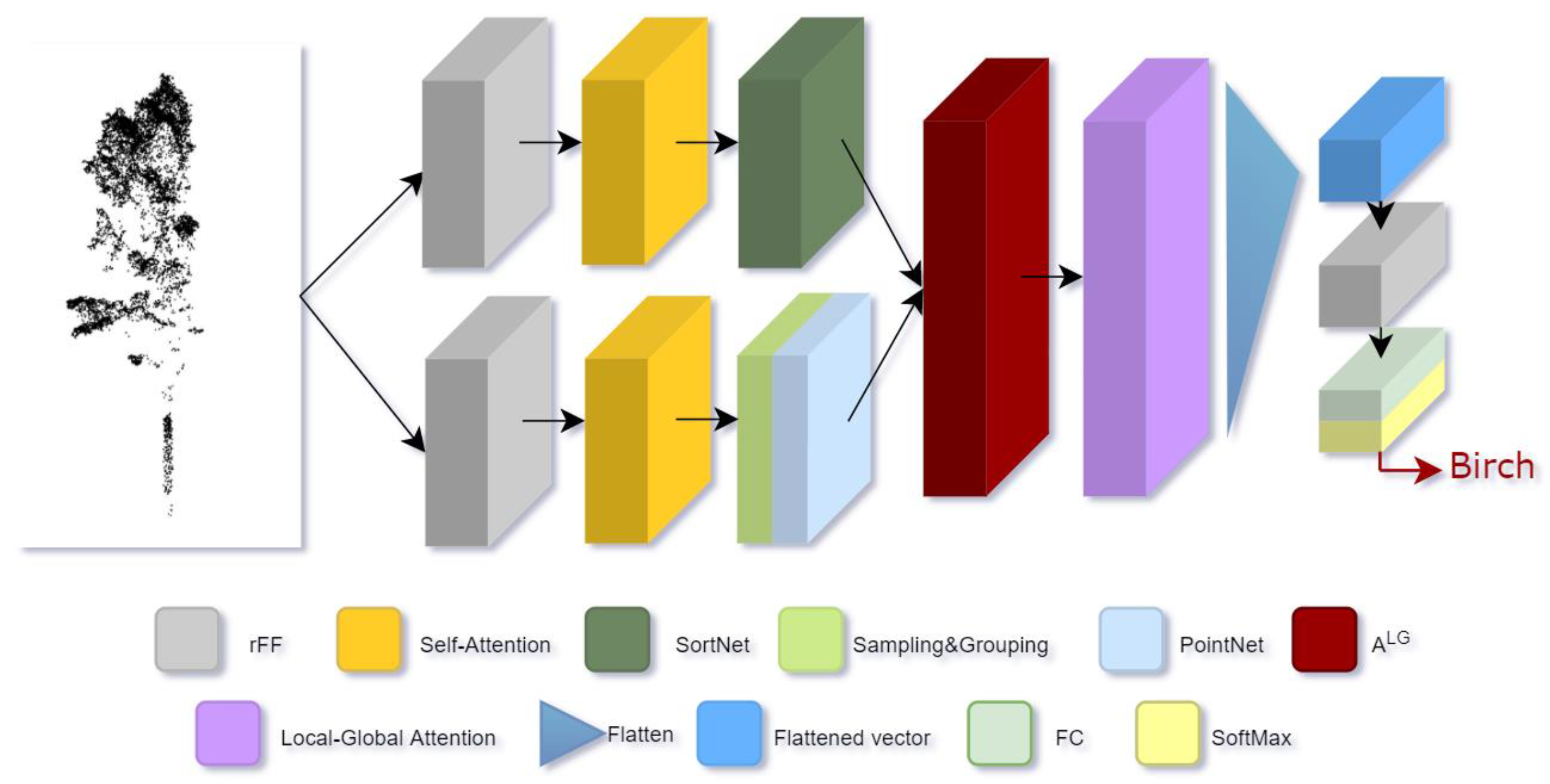
In the field of individual tree species classification, deep learning algorithms are often considered as classifiers in the workflow. The data set currently widely used as a benchmark for comparison in point cloud classification tasks is ModelNet40, which was proposed by Princeton University [28]. In order to apply the data set to the popular framework, the point cloud system of single trees segmented in this study was used as the ModelNet40-like data set.

Considering the large amount of data required for deep learning to extract features, these data were first enhanced, including rotation, mirroring, and other operations. After calculating the normal vector, a total of 2000 files were obtained for three species of trees. Additionally, in a neural network, each sample point cloud needs to have the same width, and each file needs to be resampled to ${10}^4$ points. Due to the penetration ability and accuracy of the UAV LiDAR system, the widths of the segmented tree point cloud were not all greater than ${10}^4$, meaning that we needed to resample. Additional points from up sampling were different from the original information obtained using LiDAR technology, and the information was artificially supplemented. This type of information is not always beneficial to feature extraction. In order to minimize the impact of these extra points, a multi-scale up sampling method was adopted. The width of the breakpoint cloud was determined. If the width was greater than ${10}^4$, it would not be processed. If the width was less than ${10}^4$, we set an appropriate scale according to the value of the current file. Finally, the point clouds with widths less than ${10}^4$ were upsampled to just over ${10}^4$. After up sampling, down sampling was needed in order to reduce their width to ${10}^4$ exactly. Here, the method of random sampling points was used to make the point cloud more evenly distributed. In order to make the network converge quickly, the coordinates of the point cloud were normalized and limited to the interval of $\left(-1.1\right)$. The files were converted to txt format, saved in different folders according to different labels, divided into a training set and test set according to an 8:2 ratio, and corresponding configuration files were generated by using scripts. Finally, ModelNet3 was obtained, which belongs to us. The content and division of the data set are shown in

Table 2. Data set partition.

	Quantity	Tree Species	Number of Each Species
		Birch	320
Training Set	1600	Quercus mongolica	640
		Sylvestris	640
		Birch	80
Test Set	400	Quercus mongolica	160
		Sylvestris	160

.

2.3.4. Classifier

Based on Transformer

As the pioneer of the point cloud Transformer, the PCT network architecture is shown in Figure 7. The encoder of PCT first embeds the input coordinates into the new feature space. The embedded features are input into the four stacked attention modules, the rich and discriminative representation of each point is learned, and then, the output features are generated in the linear layer.

Given an input point cloud $𝒫\in {ℝ}^{N\times d}$, where $N$ points have $d$—dimensional feature description, a $d_e$—dimension embedded feature ${\mathrm{F}}_e\in {ℝ}^{N\times d_e}$ is first learned via being input to the embedding module. The pointwise $d_o$—dimension feature from PCT is expressed as ${\mathrm{F}}_o\in {ℝ}^{N\times d_o}$, which is formed by concatenating the output of each attention layer through the feature dimension. The linear transformation formula is as follows:

$${\mathrm{F}}_1={\mathrm{AT}}^1\left({\mathrm{F}}_e\right),$$

(1)

$${\mathrm{F}}_i={\mathrm{AT}}^i\left({\mathrm{F}}_{i-1}\right), i=2, 3, 4$$

(2)

$${\mathrm{F}}_o=\mathrm{concat}\left({\mathrm{F}}_1,{\mathrm{F}}_2,{\mathrm{F}}_3,{\mathrm{F}}_4\right)·{\mathrm{W}}_o,$$

(3)

where ${\mathrm{AT}}^i$ expresses the $i$th attention layer, which has the same output and input dimensions. ${\mathrm{W}}_o$ represents the weight of the linear layer. To effectively extract global feature ${\mathrm{F}}_g$, the network applies max-pooling layer and average-pooling layer. For the classification task studied in this paper, the global feature ${\mathrm{F}}_g$ was sent to the classification decoder, which was composed of two cascaded feed-forward neural networks, LBRD (combining Linear, BatchNorm (BN), ReLU layer, and Dropout layer). The drop probability of each LBRD was 0.5. Finally, a linear layer was applied to predict the final classification score $\mathcal{C}\in {ℝ}^{N_c}$ and to determine the tree species of the point cloud among three labels using the highest score.

To prove the superiority of the Transformer better in this field, our research also used other two 3D-point transformer algorithms [29,30] proposed in the same year with PCT. The network architecture point transformer proposed by Zhao [29] is shown in Figure 8. The architecture also named point transformer proposed by Engel [30] is shown in Figure 9. In order to distinguish the two networks better, the one proposed by Zhao [29] is called PT1 and the one proposed by Engel [30] is called PT2 in the following part of this article.

Based on MLP

As the first deep learning algorithm directly acting on the point cloud, PointNet uses the global max-pooling method to extract features from all point clouds. It is effective but also leads to some problems, such as the insufficient consideration of local features. The author who proposed PointNet also proposed PointNet++, which uses PointNet to extract local features through a new grouping method. The network structure of the classification section of PointNet++ is shown in Figure 10. First, local features are extracted from small regions to capture fine geometric structures; these local features are further grouped into larger units and processed to generate higher-level features. This process is repeated until the features of the entire point set are obtained.

The core module of PointNet++ is the SA (set abstraction) module, which mainly includes the following three steps: random sampling, grouping, and feature extraction using PointNet. The SA module first uses the farthest point sampling to randomly sample points in the original point cloud and uses the sampled point as the center point to select points in the sphere within the specified radius. These points are taken as a group, features for each group are extracted via PointNet, and the global features of each group of points are obtained with max pooling.

Random Forest

The random forest (RF) has gained popularity in the field of tree species classification. RF is an integrated learning method based on decision trees, which is combined with many ensemble-regression or classification trees [31,32]. It uses decision trees for classification due to its observations. For the samples not chosen as training samples, each decision tree gives a classification result. The class is determined by decision tree votes, and the final result will be obtained by observing the maximum number of votes.

The random forest is different from the classical bagging algorithm in that it prevents the correlation between decision trees. It does not consider all the input variables (features) when building each decision tree, but only considers the random selection of these input variables. The advantage of RF is that it has relatively fast training speeds and a high level of accuracy [33]. In this study, RF was implemented in Python. As our study did not involve auxiliary information from other devices, only the original point cloud information was used as the feature of RF.

Training

The training platform used was Ubuntu 22.04, with NVIDIA GTX1080ti driven by CUDA 10.1. The sampling points of several neural networks were set to 128, 256, 512, 1024, 2048, 4096, and 8192. The Adam optimization algorithm was adopted. The batch size was set to 32, the initial learning rate was set to ${10}^{-3}$, and the weight attenuation was set to ${10}^{-3}$. A total of 600 epochs were trained.

2.3.5. Comparison and Evaluation

The separation of test and training data is very important for the evaluation of classification results. Each tree point cloud in this research was extracted using the delineation algorithm we mentioned in Section 2.3.2. Additionally, the final classification results were obtained by applying several deep learning algorithms on the test set, which was completely independent of the training set, while RF was used for simultaneous comparison. These results were then evaluated in terms of overall accuracy (OA), kappa coefficient (KC), producer’s accuracy (PA), and user’s accuracy (UA) using reference data and the confusion matrix. Additionally, the indexes we needed were calculated using the formula as follows:

$$OA=\frac{TP+TN}{TP+FN+FP+TN}\times 100\%$$

(4)

$$UA=\frac{TP}{TP+FP}\times 100\%$$

(5)

$$PA=\frac{TP}{TP+FN}\times 100\%$$

(6)

$$kappa=\frac{p_o-p_e}{1-p_e}$$

(7)

where $TP$ is the positive samples predicted by the model as positive classes, $FP$ is the negative samples predicted by the model as positive classes, $FN$ is the positive samples predicted by the model as negative classes, $TN$ is the negative samples predicted by the model as negative classes, $p_o$ is equal to OA and $p_e$ is the sum of the product of the actual sample size, and the predicted sample size is divided by the square of the total number of samples.

3. Results

3.1. Classification Results of Different Models

The models based on Transformer, MLP and random forest were used to classify Quercus mongolica, birch, and sylvestris trees, respectively. The number of sampling points was set to 4096, the most appropriate value we obtained through the experiment, and the classification results of several algorithms are shown in

Table 3. The confusion matrix of detailed classification results of each algorithm on test set.

Model	Predicted Class	True Class			Total
		Birch	Quercus mongolica	Sylvestris
	Birch	70	5	2	77
PCT	Quercus mongolica	8	138	13	159
	Sylvestris	2	17	145	164
	Birch	68	5	2	75
PT1	Quercus mongolica	8	138	16	162
	Sylvestris	4	17	142	163
	Birch	70	4	4	78
PT2	Quercus mongolica	6	142	17	165
	Sylvestris	4	14	139	157
	Birch	65	9	4	78
PN + MSG	Quercus mongolica	10	134	13	157
	Sylvestris	5	17	143	165
	Birch	63	10	2	75
PN + SSG	Quercus mongolica	9	134	15	158
	Sylvestris	8	16	143	167
	Birch	59	11	4	74
PointNet	Quercus mongolica	15	127	18	160
	Sylvestris	6	22	138	166
	Birch	50	25	19	94
RF	Quercus mongolica	16	98	36	150
	Sylvestris	14	37	105	156

. The overall accuracy and kappa coefficients of different models were obtained as shown in

Table 4. Comparison of classification accuracy of seven models.

Model	Overall Accuracy %	Kappa Coefficient
PCT	88.3	0.82
PT1	87.3	0.80
PT2	87.8	0.81
PN + MSG	85.5	0.77
PN + SSG	85.0	0.76
PointNet	80.5	0.70
RF	63.3	0.43

by analyzing the confusion matrix. In these tables, PN refers to PointNet, SSG and MSG refer to single-scale group method and multi-scale group method. The producer’s accuracy (PA) and user’s accuracy (UA), obtained in the same manner as OA and KC, are shown in Figure 11 and Figure 12. It can be observed that when only original point cloud information was used, the deep learning algorithm displayed obvious advantages over the traditional machine learning algorithm, with a high level of accuracy when classifying tree species. When evaluating the overall accuracy, the results of the three Transformer [23,29,30] point cloud classification networks were very similar to each other, being 88.3%, 87.3%, and 87.8%, respectively, slightly higher than the accuracies of 85.5% and 85.0% of the two PointNet++ grouping methods, higher than 80.5% obtained using the original PointNet, and far higher than 63.3% obtained using RF. Among the seven algorithms implemented, PCT displayed the best effect, with the kappa coefficient reaching 0.82, which was 0.12 and 0.39 greater than PointNet and RF, respectively.

As the results of PA and UA showed, these algorithms performed differently in each class. Considering the index of UA, the accuracy of birch was generally slightly lower than that of Quercus mongolica, and the effect of identifying sylvestris was better. PCT performed best in the category of birch and sylvestris, reaching 87.5% and 90.7%. Point Transformer proposed by Engle et al. [30] performed best in the category of Quercus mongolica, reaching 88.75%. Meanwhile, the same index performed worst using RF; this would make it difficult to apply it to practical problems. On the other hand, producer’s accuracy values indicated that there was no obvious difference in classification performance among the three tree species. The PCT algorithm performed best in the classification tasks of the three tree species, and the producer’s accuracy reached 91.0%, 86.8%, and 88.4%, respectively.

3.2. Classification Results of Different Sample Point Densities

For different sample point densities, the overall accuracy trends of the corresponding classification with the number of sampling points are shown in Figure 13. It can be seen that in the dimension of sample point density, with the increase in the number of sampling points, the overall accuracy of several algorithms gradually increased and showed trends of rapid growth and then slow growth. However, the growth trend slowed down when the number of sampling points reached 4096, and the overall accuracy of PointNet++ using MSG decreased slightly when the number of sampling points reached 8192.

In addition, the differences in the overall accuracy among different algorithms was less affected by the number of sampling points. Additionally, under other sampling points, they were similar to the previous results; that is, three Transformer-based classification algorithms had slightly higher overall accuracy values than several MLP-based PointNet families.

4. Discussion

4.1. Comparison of Different Models

After our test, it was shown that PCT achieved the best classification accuracy, and the other two Transformer-based deep learning algorithms had similar effects. In addition, the most primitive PointNet based on MLP performed worst in several models. Although the max-pooling layer is used to solve point cloud disorder, due to the limitation of its structure, it can only extract global features, not local features. It has limited ability in detail processing and generalization to complex scenes [19]. In contrast, PointNet++ has an additional multi-scale or multi-resolution grouping structure, which solves the problem of uneven density distribution in a point cloud. In particular, the point cloud density of a tree crown from the UAV LiDAR system was higher than that of the under forest [34], which was more obvious. However, in the field of irregular domain and unstructured point cloud learning, the Transformer-based PCT showed better performance [23], such as in the tree species classification task, with little morphological difference between classes. PCT was shown to have the highest classification accuracy for each tree species (90% for sylvestris), and each species showed similar accuracy because PCT is based on Transformer rather than using a self-attention mechanism as an auxiliary module. The results show that PCT is very suitable for tree species classification. For comparison, Liu et al. [18] used LiDAR data and the neural network built by his team to classify the two species. The maximum OA was 86.7%, slightly lower than the PCT we used. Our study area is located in a park with flat terrain, and trees are planted and cared for by gardeners. In addition, compared with a natural forest with rich species and disorder, the tree distribution in our study had a certain pattern and was easy to classify. Therefore, the accuracy in artificial forest prediction will be higher.

4.2. Comparison of Different Tree Species

Liu et al. [18] selected two trees with large morphological differences as experimental objects: white birch, which is a broad-leaved tree, and larch, which is a coniferous tree. Therefore, we selected sylvestris, birch, and Quercus mongolica in our research. Two of these are broad-leaved trees, and one is a coniferous tree, which meant we could distinguish the performance of broad-leaved forests in the same network. The classification accuracy of PCT for each tree species was the highest and showed similar accuracy, being higher than 86%. However, according to the classification results of several models, there were slight differences in the classification accuracy of different tree species, which generally showed that the classification accuracy was lower than the others on Quercus mongolica, while it performed better on sylvestris and birch. To explain this phenomenon, three tree point cloud image samples are shown in Figure 14.

The images show that the shape of sylvestris and birch are unique and show obvious differences, but the difference between Quercus mongolica and the other two trees are not obvious. Especially because of the dense planting and high canopy density within Quercus mongolica forest, the airborne LiDAR technology could not penetrate the forest well, and the trunk information density obtained was relatively low. Therefore, as the only coniferous tree, sylvestris had the highest classification accuracy, while several algorithms on Quercus mongolica generally performed relatively poorly. The features extracted from Quercus mongolica by the network were similar to each other, and there were more misclassifications. This finding is similar to the conclusions drawn in the field of tree classification using 2D images. Liu et al. [35] concluded that higher classification accuracy is achieved with coniferous trees with obvious crown structures. Compared with coniferous trees, deciduous tree crowns are denser, and the gaps between the tree crowns are smaller. Inaccurate crown delineation will reduce the differences among the point cloud of three tree species and lead to more misclassification.

4.3. Influence of Sample Point Density on Classification Results

For LiDAR data, the deep learning method we used contained sampling modules. We used different sampling points during training, as shown in Figure 10. As the number of sampling points increased from 128 to 4096, the classification accuracy gradually improved. When the number of sampling points in each tree exceeded 4000, the classification performance of the network tended to be saturated. The reason why the increase in point density greatly improved the classification effect at the initial stage is that the similarity between different tree species was high, and with the increase in point density more geometric structure information could be retained so that the network could learn more features. When the number of sampling points increased to 8096, the classification accuracy of PointNet++ using multi-scale grouping decreased. This is because the point density was too large and the extracted information was redundant, resulting in low classification accuracy. If the point density was too large, the number of model parameters could not be increased resulting in the slow convergence speed in model training, which affected the accuracy of the test.

4.4. Comparison with Machine Learning Model

Spectral, texture, and shape features are usually extracted for tree species classification using machine learning methods such as RF and support vector machines. These features and classifiers have been widely used in similar research [36,37]. In our study, the RF algorithm was adopted to classify the point cloud data based on the elevation information, reflection intensity, curvature, and color. Two parameters were adjusted. The number of trees, created by randomly selecting samples from the training samples, and the number of variables, used for tree node splitting were modified for RF. The number of trees defaulted to 500, and the number of variables defaulted to the square root of the number of input features. Belgiu et al. [32] believed that the default parameter value was effective; therefore, we adopted the default value. The results show that the effect of classification by using the original point cloud information alone is very unsatisfactory. The overall accuracy of RF was only 63.3%, which is far lower than several deep learning algorithms. This is because the original point cloud contained too little information for machine learning and required manual feature selection. Without the assistance of other equipment, such as a hyperspectral camera, the task cannot be completed to a high standard by only using a few features. On the contrary, deep learning algorithms abstract the features, simplify the feature extraction, and can better classify the tree species.

5. Conclusions

In our study, airborne LiDAR point cloud data are used to explore the potential of Transformer in the field of 3D tree point cloud classification in recent years based on the delineation algorithm, and several existing classification methods were compared. Several deep learning models were evaluated using OA, KC, PA, and UA. The accuracy of several models was also compared with the random forest algorithm, which only uses elevation information, reflection intensity, curvature, and color features. In this paper, we used the clustering algorithm to segment the preprocessed point cloud data into single trees, and we took single tree point clouds obtained as the input of the classifier. Like other scholars who used 3D deep learning algorithms, we showed that the method we applied can directly train point cloud data samples to derive the model. This experiment proves the validity of this method in 3D tree species classification. Considering the comparison of the performance of different models on our own data set, the classification accuracy of PCT was the highest, with the overall accuracy reaching 88.3% and the kappa coefficient reaching 0.82.

In addition, the classification results of different tree species and the influence of different sample density levels on classification accuracy were studied. Among Quercus mongolica, birch, and sylvestris, the classification performance of Quercus mongolica was shown to be barely satisfactory, while the performance of sylvestris was the best because the point cloud under forest was too sparse due to the excessive canopy density in the forest area, and its features could not be extracted well. With the increase in the sample point density, the classification accuracy rate continually improved, but there was a critical value to this improvement. When the number of sample points was set to 4096, the model performed best on our data set. In future work, in order to solve these problems, we will attempt to combine multi-source LiDAR technology to obtain better results; we will also attempt to apply our method to the classification of natural forest species in more complex situations.

References

1. Jarvis, P.G.; Dewar, R.C. Forests in the Global Carbon Balance: From Stand to Region. In Scaling Physiological Process: Leaf to Globe; Ehleringer, J.R., Field, C.B., Eds.; Academic Press: Cambridge, MA, USA, 1993; pp. 191–221. [Google Scholar]
2. McRoberts, R.E.; Cohen, W.B.; Naesset, E. Using remotely sensed data to construct and assess forest attribute maps and related spatial products. Scand. J. For. Res. 2010, 25, 340–367. [Google Scholar] [CrossRef]
3. Næsset, E.; Gobakken, T.; Holmgren, J. Laser scanning of forest resources: The Nordic experience. Scand. J. For. Res. 2004, 19, 482–499. [Google Scholar] [CrossRef]
4. Lechner, A.M.; Foody, G.M.; Boyd, D.S. Applications in remote sensing to forest ecology and management. One Earth 2020, 2, 405–412. [Google Scholar] [CrossRef]
5. Wulder, M.A.; White, J.C.; Nelson, R.F. Lidar sampling for large-area forest characterization: A review. Remote Sens. Environ. 2012, 121, 196–209. [Google Scholar] [CrossRef] [Green Version]
6. Seidel, D.; Ehbrecht, M.; Annighöfer, P. From tree to stand-level structural complexity-which properties make a forest stand complex? Agric. For. Meteorol. 2019, 2781, 07699. [Google Scholar] [CrossRef]
7. Abd Rahman, M.Z.; Gorte, B.G.H.; Bucksch, A.K. A new method for individual tree delineation and undergrowth removal from high resolution airborne lidar. In Proceedings of the ISPRS Workshop Laserscanning 2009, Paris, France, 1–2 September 2009; Volume XXXVIII. Part 3/W8. [Google Scholar]
8. Qi, W.; Dubayah, R.O. Combining Tandem-X InSAR and simulated GEDI lidar observations for forest structure mapping. Remote Sens. Environ. 2016, 187, 253–266. [Google Scholar] [CrossRef]
9. Brandtberg, T.; Warner, T.A. Detection and analysis of individual leaf-Off tree crowns in small footprint, high sampling density LIDAR data from the eastern deciduous forest in North America. Remote Sens. Environ. 2003, 85, 290–303. [Google Scholar] [CrossRef]
10. Cao, J.; Leng, W.; Liu, K. Object-based mangrove species classification using unmanned aerial vehicle hyperspectral images and digital surface models. Remote Sens. 2018, 10, 89. [Google Scholar] [CrossRef] [Green Version]
11. Li, J.; Hu, B.; Noland, T.L. Classification of tree species based on structural features derived from high density LiDAR data. Agric. For. Meteorol. 2013, 171, 104–114. [Google Scholar] [CrossRef]
12. Kim, S.; McGaughey, R.J.; Andersen, H.E. Tree species differentiation using intensity data derived from leaf-on and leaf-off airborne laser scanner data. Remote Sens. Environ. 2009, 113, 1575–1586. [Google Scholar] [CrossRef]
13. Shoot, C.; Andersen, H.E.; Moskal, L.M. Classifying forest type in the national forest inventory context with airborne hyperspectral and lidar data. Remote Sens. 2021, 13, 1863. [Google Scholar] [CrossRef]
14. Alonzo, M.; Bookhagen, B.; Roberts, D.A. Urban tree species mapping using hyperspectral and lidar data fusion. Remote Sens. Environ. 2014, 148, 70–83. [Google Scholar] [CrossRef]
15. Sun, Y.; Huang, J.; Ao, Z. Deep learning approaches for the mapping of tree species diversity in a tropical wetland using airborne LiDAR and high-spatial-resolution remote sensing images. Forests 2019, 10, 1047. [Google Scholar] [CrossRef] [Green Version]
16. Mizoguchi, T.; Ishii, A.; Nakamura, H. Individual tree species classification based on terrestrial laser scanning using curvature estimation and convolutional neural network. Int. Arch. Photogramm. Remote Sens. Spat. Inf. Sci. 2019, XLII-2/W13, 1077–1082. [Google Scholar] [CrossRef] [Green Version]
17. Xi, Z.; Hopkinson, C.; Rood, S.B. See the forest and the trees: Effective machine and deep learning algorithms for wood filtering and tree species classification from terrestrial laser scanning. ISPRS J. Photogramm. Remote Sens. 2020, 168, 1–16. [Google Scholar] [CrossRef]
18. Liu, M.; Han, Z.; Chen, Y. Tree species classification of LiDAR data based on 3D deep learning. Measurement 2021, 177, 109301. [Google Scholar] [CrossRef]
19. Qi, C.R.; Su, H.; Mo, K. Pointnet: Deep learning on point sets for 3d classification and segmentation. In Proceedings of the IEEE Conference on Computer Vision and Pattern Recognition, Honolulu, HI, USA, 21–26 July 2017; pp. 652–660. [Google Scholar]
20. Qi, C.R.; Yi, L.; Su, H. Pointnet++: Deep hierarchical feature learning on point sets in a metric space. Adv. Neural Inf. Process. Syst. 2017, 30, 5105–5114. [Google Scholar]
21. Vaswani, A.; Shazeer, N.; Parmar, N. Attention is all you need. Adv. Neural Inf. Process. Syst. 2017, 30, 1–15. [Google Scholar]
22. Pang, Y.; Wang, W.; Tay, F.E.; Liu, W. Masked autoencoders for point cloud self-supervised learning. arXiv 2022, arXiv:2203.06604. [Google Scholar]
23. Guo, M.H.; Cai, J.X.; Liu, Z.N. Pct: Point cloud transformer. Comput. Vis. Media 2021, 7, 187–199. [Google Scholar] [CrossRef]
24. Zhang, W.; Qi, J.; Wan, P. An easy-to-use airborne LiDAR data filtering method based on cloth simulation. Remote Sens. 2016, 8, 501. [Google Scholar] [CrossRef]
25. Lu, X.; Guo, Q.; Li, W. A bottom-up approach to segment individual deciduous trees using leaf-off lidar point cloud data. ISPRS J. Photogramm. Remote Sens. 2014, 94, 1–12. [Google Scholar] [CrossRef]
26. Véga, C.; Hamrouni, A.; el Mokhtari, S. PTrees: A point-based approach to forest tree extraction from lidar data. Int. J. Appl. Earth Obs. Geoinf. 2014, 33, 98–108. [Google Scholar] [CrossRef]
27. Shendryk, I.; Broich, M.; Tulbure, M.G. Bottom-up delineation of individual trees from full-waveform airborne laser scans in a structurally complex eucalypt forest. Remote Sens. Environ. 2016, 173, 69–83. [Google Scholar] [CrossRef]
28. Wu, Z.; Song, S.; Khosla, A. 3d shapenets: A deep representation for volumetric shapes. In Proceedings of the IEEE Conference on Computer Vision and Pattern Recognition, Boston, MA, USA, 7–12 June 2015; pp. 1912–1920. [Google Scholar]
29. Zhao, H.; Jiang, L.; Jia, J. Point transformer. In Proceedings of the IEEE/CVF International Conference on Computer Vision, Montreal, BC, Canada, 11–17 October 2021; pp. 16259–16268. [Google Scholar]
30. Engel, N.; Belagiannis, V.; Dietmayer, K. Point transformer. IEEE Access 2021, 9, 134826–134840. [Google Scholar] [CrossRef]
31. Breiman, L. Random forests. Mach. Learn. 2001, 45, 5–32. [Google Scholar] [CrossRef] [Green Version]
32. Belgiu, M.; Drăguţ, L. Random forest in remote sensing: A review of applications and future directions. ISPRS J. Photogramm. Remote Sens. 2016, 114, 24–31. [Google Scholar] [CrossRef]
33. Liaw, A.; Wiener, M. Classification and Regression by randomForest. R News 2002, 2, 18–22. [Google Scholar]
34. Brede, B.; Lau, A.; Bartholomeus, H.M. Comparing RIEGL RiCOPTER UAV LiDAR derived canopy height and DBH with terrestrial LiDAR. Sensors 2017, 17, 2371. [Google Scholar] [CrossRef]
35. Liu, L.; Coops, N.C.; Aven, N.W. Mapping urban tree species using integrated airborne hyperspectral and LiDAR remote sensing data. Remote Sens. Environ. 2017, 200, 170–182. [Google Scholar] [CrossRef]
36. Sothe, C.; De Almeida, C.M.; Schimalski, M.B. Comparative performance of convolutional neural network, weighted and conventional support vector machine and random forest for classifying tree species using hyperspectral and photogrammetric data. GIScience Remote Sens. 2020, 57, 369–394. [Google Scholar] [CrossRef]
37. Hartling, S.; Sagan, V.; Sidike, P. Urban tree species classification using a WorldView-2/3 and LiDAR data fusion approach and deep learning. Sensors 2019, 19, 1284. [Google Scholar] [CrossRef] [PubMed] [Green Version]
Figure 1. (a)The location map of the study area; (b) aerial view of the study area.
Forests 14 00484 g001
Figure 2. The side view of collected point cloud file with no color.
Forests 14 00484 g002
Figure 3. The flowchart of the proposed method.
Forests 14 00484 g003
Figure 4. The rendering of denoising step. There are plenty of noise points above the forest before denoising while there are not much after denoising.
Forests 14 00484 g004
Figure 5. (a) Results of separating ground points; (b) results of separating non-ground points.
Forests 14 00484 g005
Figure 6. The results of segmentation algorithm: the left shows the algorithm demonstration of a small batch of samples, and the right figure shows part of the segmentation results, which is rendered into different colors to distinguish individual trees.
Forests 14 00484 g006
Figure 7. The architecture of PCT. LBR represents the linear layer, BatchNorm layer, and ReLU layer; MA pool layer represents the maximum pooling layer and average pooling layer; and LBRD represents the linear layer, BatchNorm layer, ReLU layer, and Dropout layer.
Forests 14 00484 g007
Figure 8. The architecture (PT1) proposed by Zhao [29], including mlp, point transformer block, transition down block, and global average pooling, where N refers to input point numbers. The transition down module is to reduce the cardinality; the point transformer is the core module to output features.
Forests 14 00484 g008
Figure 9. The architecture proposed (PT2) by Engel [30]. rFF represents row-wise feed-forward network, SortNet is a local feature generation module, A L G generate local-global attention by relating global features with local features, and FC represents fully connected layer.
Forests 14 00484 g009
Figure 10. The classification section of structure of PointNet++.
Forests 14 00484 g010
Figure 11. PA (producer’s accuracy) bar chart of seven algorithm calculated from confusion matrix.
Forests 14 00484 g011
Figure 12. UA (user’s accuracy) bar chart of seven algorithm calculated from confusion matrix.
Forests 14 00484 g012
Figure 13. (a) Schematic diagram of farthest point sampling algorithm affected by point density; (b) the overall accuracy of different deep learning algorithms increases with an increase in the number of sampling points.
Forests 14 00484 g013
Figure 14. From left to right, the species of tree point cloud is birch (a), Quercus mongolica (b), and sylvestris (c).
Forests 14 00484 g014