The Relationship between Socioeconomic Factors at Different Administrative Levels and Forest Fire Occurrence Density Using a Multilevel Model

Abstract

Wildfires are among the main factors that disturb terrestrial ecosystems, landscapes, and the environment. Understanding the differences that the socioeconomic factors of different administrative levels have on fire occurrence remains critical to inform the driving function of ignition sources. In this study, we collected socioeconomic and land use data for 21 cities and 81 counties in the study area from 2001 to 2019 and applied a multilevel model to explore the relationship between wildfire occurrence density and the driving factors. We estimated the fixed and random effect of the factors at different levels and built three hierarchical linear models (HLMs) to quantify the impacts of socioeconomic drivers on wildfires. The results showed that the variance among cities contributed to 14.01% of the unexplained variation of random effects at the county level. At the county level, the densities of middle school student populations, gross domestic product (GDP), and impervious surface areas were significantly positively correlated with fire occurrence density. At the city level, GDP and its interaction with county-level factors were significantly negatively correlated with fire occurrence density. This study provides a new method and findings for the research of wildfire occurrence and risk.

1. Introduction

Wildfire is an important disturbance factor in terrestrial ecosystems and plays a key role in mediating the structure, function, and evolutionary succession of the ecosystem while also exerting a significant impact on the global carbon cycle and climate change [1,2,3,4]. Especially in fire-adapted ecosystems, such as dry pine, dry coniferous mixed forest, grassland, savanna, etc., wildfire has become a component of these ecosystems for the maintenance, restoration, and succession of the landscape [5,6,7,8,9]. With global climate change, the length of the fire season and fire weather have been substantially prolonged, leading to a great increase in fire occurrence [10,11]. It is predicted that the frequency and intensity of wildfires will further increase in the coming decades [11,12,13].

Wildfires are the result of the interaction of multiple factors at different spatial and temporal scales [14,15]. Vegetation, climate, and ignition source are the major fire drivers that determine the spatial and temporal patterns of wildfires [16,17,18,19,20]. Analyzing the causes of wildfire occurrence and wildfire dynamics is the basis for estimating fire risk, fire behavior, and related consequences [21,22,23,24,25]. Wildfires can be classified into two categories on the basis of the type of ignition material. These are natural fires and anthropogenic fires. Natural fires are mainly caused by lightning [22,26,27], while anthropogenic fires are more common around the world and are strongly associated with human activities [28,29,30].

Some ordinary activities and factors that may potentially lead to wildfires include picnics, children playing with fire, festivals, smoking, cooking, deregulation, etc. [31,32,33,34,35]. However, it is difficult to accurately quantify the extent to which human factors (i.e., major fire ignition sources) contribute to wildfire because most factors are difficult to predict at the landscape scale [36]. Some previous studies used socioeconomic factors (such as population, gross domestic product, number of students) and land use factors (e.g., area of forest, settlement and field pattern, length and density of roads) to represent the ignition factors [35,37,38,39,40,41,42,43,44]. In these studies, socioeconomic data and land use data representing fire ignition sources are mainly analyzed, and good results were achieved, by taking administrative regions as the statistical units to explore the distribution pattern of anthropogenic fires [33,40,41,43,45].

Other studies also analyzed the relationship between wildfire and drivers using a specific unit or a single geographical scale to quantify wildfire distributions and evaluate fire risks [25,46,47,48,49]. In some cases, county scale, prefecture-level city scale, or ecological region scale are ideal scales to analyze the effect of factors on the occurrence of wildfires [25,50,51,52,53]. However, wildfire ignitions and human activities are clustered on different spatial scales [54]. Modeling relationships between socioeconomic factors and wildfires at a single spatial scale only cannot completely explore the local variability among related factors. Such methods take the samples as a group to analyze the average set of results, ignoring some potential spatial variation across different spatial scales. Additionally, these methods also minimized the spatial variability due to data distribution, random samples, and regional differences (such as environmental background differences), and ignored the variable bias in different statistical units [55]. It is difficult to understand human behavior without considering its context, and the effects of variables at different scales on wildfire may be confounded.

The relative relationships between human factors and fire occurrence also vary with the change in spatial scales [14,56,57]. The impact of the overall regional characteristics on wildfires can be effectively identified at larger scales, and the spatial variations of drivers within the region can be detailed at smaller scales. Unfortunately, traditional correlation-based methods are still limited when explaining the interaction between multilevel factors. The multilevel model provides a flexible and effective quantitative method to model individual and grouped data from different scales or levels and to analyze the relationship between variables that vary depending on the environmental background. This method solves the problem that arises from the traditional mathematical models; namely that those models cannot explain the spatial variability of the relationships due to different aggregation characteristics of variables at different levels [55].

In this study, we built a multilevel model that considered the spatial changes in wildfire drivers at different levels to understand how socioeconomic variables at local (county level) and higher (prefecture level) scales impact the distribution of wildfires. Additionally, this work estimates how the impacts of different levels interact to affect wildfire distribution. This study aims to explore the extent that spatial variation in fire occurrence is caused by socioeconomic factors at the county level and the prefecture level. The analysis of the spatial relationship between socioeconomic activities and wildfire occurrence can enrich the research of the impact factors of wildfire occurrence and risk.

2. Materials and Methods

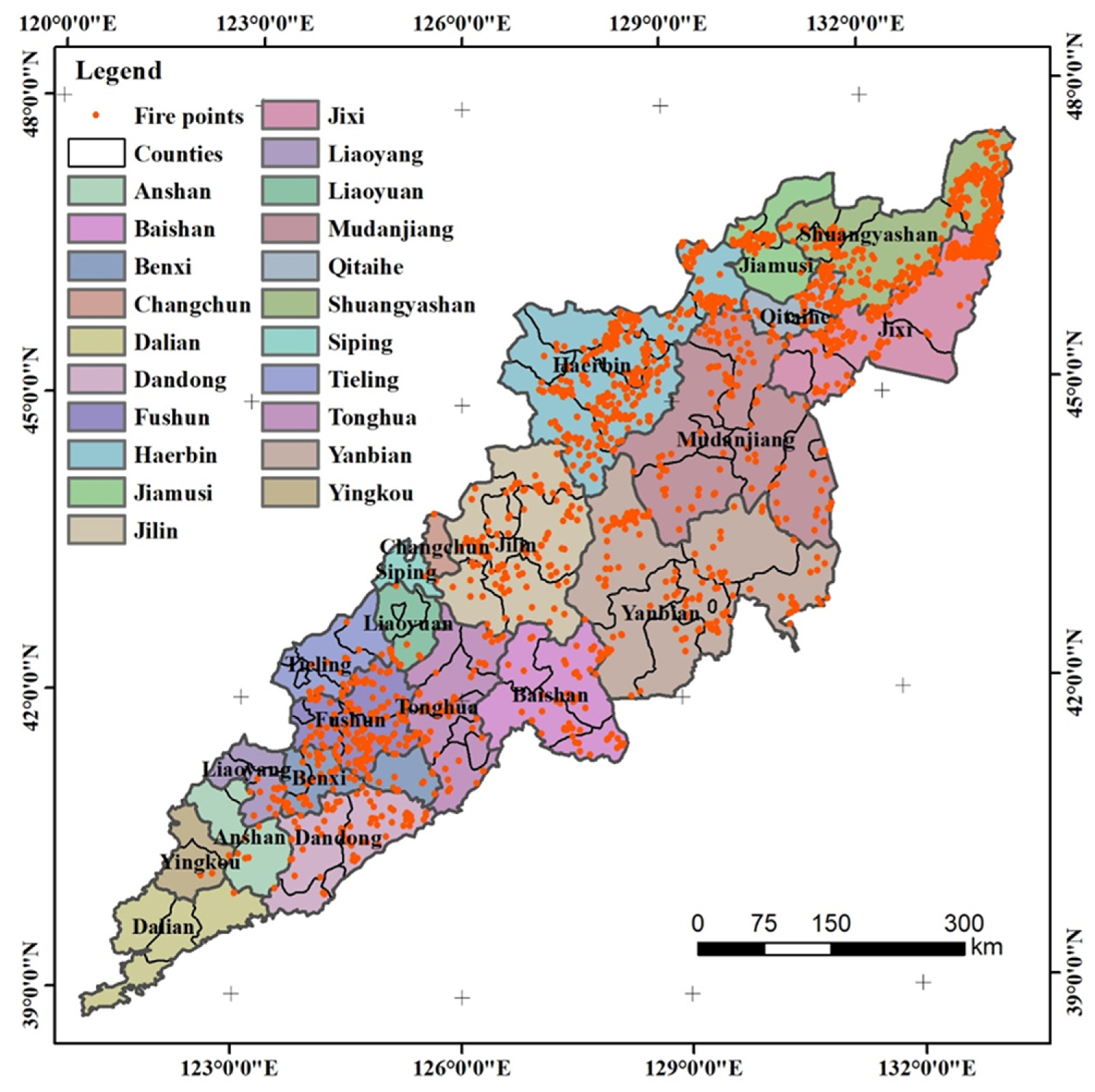
2.1. Study Area

The study area is the Changbai Mountain range, located in the eastern mountainous area of the Liaoning, Jilin, and Heilongjiang provinces of China, between 38°46′–47°30′ N and 121°08′–134° E (Figure 1). It starts from Wanda Mountain in the north and extends to Qianshan Mountain in the south, is approximately 1300 km long from north to south, and 400 km wide from west to east. The elevation of the study areas ranges from 500 to 1000 m, and some mountain regions exceed 1000 m. The highest peak, General Peak, is 2749.2 m in elevation and is one of the mountains in the east of the Asian continent. The climate of Changbai Mountain is a temperate continental monsoon climate, with the general characteristics of cold winters, warm summers, dry springs, and cool autumns. The average annual temperature is between −7 °C and 3 °C. The average temperature in July is close to 10 °C, and in January, it is approximately −20 °C. The annual precipitation is 700–1400 mm, and the precipitation from June to September accounts for 60%–70% of the annual rainfall.

Forest constitutes the largest land use/land cover type in the region, accounting for approximately 59% of the study area. Temperate coniferous and broad-leaved mixed forest comprise the main vegetation types. The second most abundant land use type is cropland, which accounts for approximately 35% of the study area. Other types are grassland, shrub, wetland and water bodies, bare land, and artificial surfaces. Perennial snow cover only appears sporadically at the top of the highest peak. The region spans 3 provinces, 21 prefecture-level cities, and 82 counties, which are all socioeconomically active. Forest wildfires in this region occur mainly in spring and autumn, with small burned areas and long fire intervals.

2.2. Data

2.2.1. Forest Fire Points

The MOD14A1/MYD14A1 (collection 6) dataset derived from the MODIS (Moderate-Resolution Imaging Spectroradiometer) satellite provides daily active fire mask composite products with 1 km spatial resolution [58]. The active fire product data covering the study area span from January 2001 to December 2019 and were downloaded from the Level-1 and Atmosphere Archive & Distribution System (LAADS) Distributed Active Archive Center (DAAC) (https://ladsweb.mod-aps.eosdis.nasa.gov/ (accessed on 12 August 2022)). The MODIS Reprojection Tool (MRT) tool was used for image mosaicking, extraction, projection information, and processing to obtain the thermal anomaly data, which is superimposed with the forested areas to extract the forest fire pixel information for the study site. The annual fire occurrence density of each county was calculated according to the number of annual active fire points.

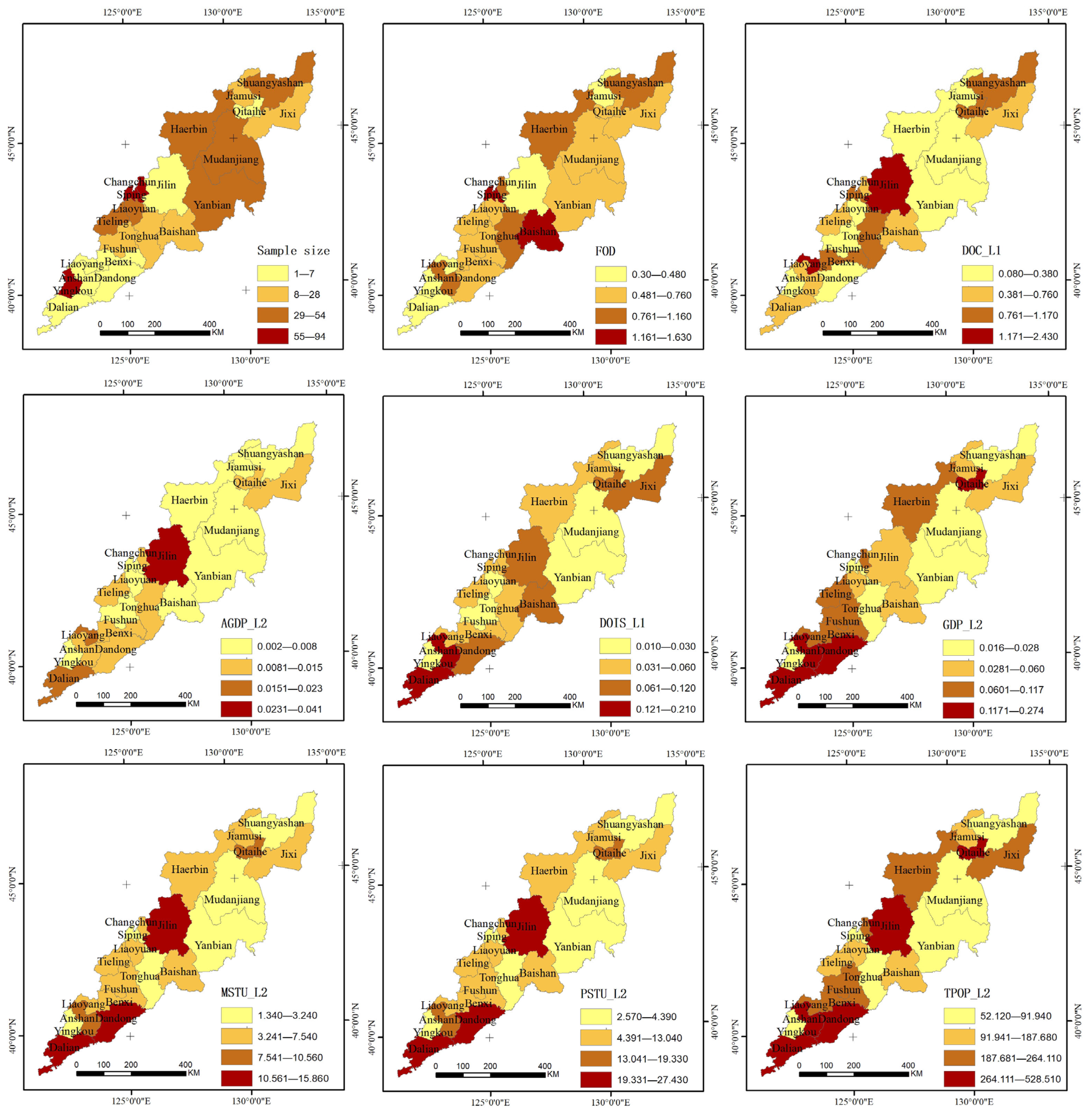
2.2.2. Socioeconomic Data and Land Use Data

The variables used in the model in this study were selected based on the results of previous studies [43,59,60]. The probability of fire occurrence has a strong correlation with variables related to human activity and accessibility [61]. Therefore, we chose the density of the total population, gross domestic product (GDP), and agricultural GDP as human activity-related variables, and the density of the impervious areas and cropland areas as human accessibility-related variables. In addition, Grala et al. [62] found that wildfires caused by children were likely to occur in densely populated areas. Moreover, many studies have found that fires caused by children were an important source of wildfire occurrence [31,62]. Also, the number of students was positively correlated with the population size, thus the number of students could also reflect the spatial distribution of the total population.

The total population, number of middle school students, number of primary school students, GDP, and agricultural GDP of 21 prefecture-level cities and 85 counties ranging from 2001 to 2019 were obtained from the statistical yearbook to represent the socioeconomic conditions of each administrative region. The 30 m spatial resolution land use/land cover data (Landsat-derived annual China land cover dataset, CLCD) from 2001 to 2019 were obtained from the following website: (http://doi.org/10.5281/zenodo.4417809 (accessed on 18 September 2022)). The impervious areas and cropland areas were extracted to calculate their coverage and proportion in each county. These socioeconomic and land use data were used as human ignition sources to analyze the impact of anthropogenic factors on forest fires at different spatial scales.

The socioeconomic data were organized into two datasets in this study (

Table 1. Summary of variables for modeling.

Level	Variable name	Abbreviation	Unit
1	Fire occurrence density	FOD_L1	times/1000 km2
1	The density of the cropland	DOC_L1	km2/km2
1	The density of the impervious surface area	DOIS_L1	km2/km2
2	The density of the total population	TPOP_L2	person/km2
2	The density of middle school students	MSTU_L2	person/km2
2	The density of primary school students	PSTU_L2	person/km2
2	The density of GDP	GDP_L2	108 yuan/km2
2	The density of agricultural GDP	AGDP_L2	108 yuan/km2

). The city-level dataset contained annual average data from 2001 to 2019 for 21 cities. These data included the total population density (TPOP_L2), density of middle school students (MSTU_L2), density of primary school students (PSTU_L2), gross domestic product density (GDP_L2), and density of agricultural GDP (AGDP_L2) of each city. The county-level dataset contained data for the same variables spanning 85 counties over 19 years (the abbreviations of these county-level variables were TPOP_L1, MSTU_L1, PSTU_L1, GDP_L1, and AGDP_L1). In addition to these data, the fire occurrence density (FOD_L1), cropland density (DOC_L1), and impervious surface area (DOIS_L1) of each county in each year were included in the study. The fire occurrence density of each county in each year was used as the dependent variable in the county-level dataset.

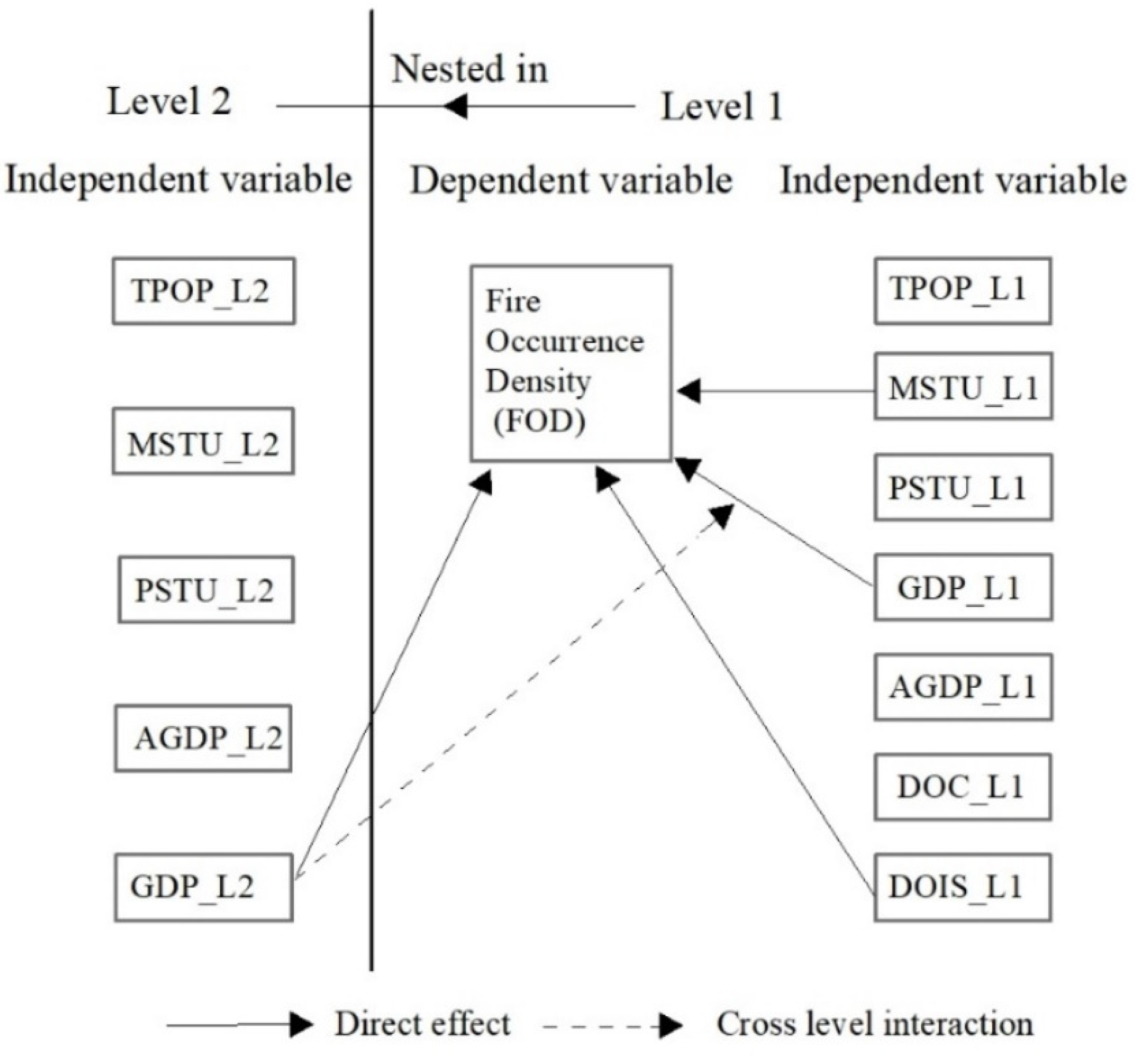
2.3. Multilevel Model

The hierarchical linear model (HLM), also known as a multilevel model (MLM), has been widely used with nested data to examine the effects of group-level and individual-level covariates on the outcomes at an individual level [63,64,65]. The HLM is mainly used in socioeconomic research, such as public health research [63], education research [66], hospitality research [67], etc. The model could analyze the impact of different levels/degrees of nested factors/data on the research objectives. For more details on the specific algorithm of the hierarchical linear model, see Raudenbush and Bryk [68].

Currently, the analyses of influencing factors in wildfire research were always carried out spatially related to fire distribution patterns at different scales, and the analyses of nested relationships between different levels of influencing factors were rarely conducted, which made it difficult to further explore the causes of the aggregation characteristics of the spatial distribution of wildfire occurrence. Applying the HLM to study the relationship between different levels of socioeconomic factors and fire occurrence could improve the existing single-scale analysis, as well as, partially, address the multiscale and cross-scale driving effects from different levels of socioeconomic factors on the distribution patterns of wildfire occurrence. There are fewer researches applying multilevel models to study fire.

Socioeconomic data are almost always inherently nested, and issues related to socioeconomic data reflect the understanding of the interaction between different levels. For example, the county level is nested at the city level, the city level at the province level, and so on. The potential effects of heterogeneity among group-level regions (such as cities) on individual-level variables can be addressed using an HLM following three steps:

First, a variance component model (null model) was fit to examine how much variance can be explained by clustering the fire occurrence density of counties within city-level regions. This null model is only used to estimate the difference in fire occurrence density between and within city regions, without considering explanatory variables. The variance component model formula was as follows:

$$\begin{gathered} \mathrm{Level} 1 \left(\mathrm{County}\right): \mathit{Y}={\mathit{\pi }}_0+\mathit{e}\dots \\ \mathrm{Level} 2 \left(\mathrm{City}\right): {\mathit{\pi }}_0={\mathit{\gamma }}_{00}+{\mathit{u}}_0, \\ \mathrm{Combined} \mathrm{model}: \mathit{Y}={\mathit{\gamma }}_{00}+{\mathit{u}}_0+\mathit{e}, \mathit{e} ~\mathit{N}\left(0, {\mathit{\sigma }}_{{\mathit{e}}_0}^2\right), {\mathit{u}}_0 ~\mathit{N}\left(0,{\mathit{\sigma }}_{{\mathit{u}}_0}^2 \right) \end{gathered}$$

(1)

where $Y$ is the forest fire occurrence density in each county and city region; ${\gamma }_{00}$ is the intercept, that is, the overall mean of $Y$ across all groups (cities); $u_0$ is the difference between the average fire occurrence density in each group (city) and the global average fire occurrence density among all regions; $e$ is the difference between $Y$ and the average fire occurrence density in each region; and ${\sigma }_{u_0}^2$ and ${\sigma }_{e_0}^2$ are the variations between and within regions. These residuals at the city and county levels are assumed to follow normal distributions. This model indicates that the fire occurrence density of the county is a function of the mean fire occurrence density in the cities and some variation in the county.

The intraclass correlation index (ICC) was used to account for the variance in fire occurrence density at the city level. That is, if only 1% of the overall variance is at the city level, the significant variables at the city level can explain at most 1% of the variance in the model results. With the variance component model, the ICC is defined as follows:

$$ICC=\frac{{\sigma }_{u_0}^2}{{\sigma }_{u_0}^2+{\sigma }_{e_0}^2}$$

(2)

where ${\sigma }_{u_0}^2$ is the variance among the city-level regions and ${\sigma }_{e_0}^2$ is the variance among the county-level regions within the same city region. The ICC value is between 0 and 1. A high ICC value indicates that city-level regions are very important for explaining the difference in fire occurrence density in counties; however, when the ICC value is very small, the difference in the results cannot be attributed to the characteristics of the city-level region [69].

Second, HLM provided a better estimation of the effects of county variables (individual level) when considering the differences between cities (group level). By including explanatory variables at the county level, the variance component model was extended to the random intercept model to estimate fixed effects. The intercepts of the region regression lines may vary randomly between regions [63]. The random intercept and random/fixed slope model can be formulated as follows:

$$\begin{gathered} \mathrm{Level} 1 \left(\mathrm{County}\right): Y={\pi }_0+{\pi }_i{X}_i+e, \\ \mathrm{Level} 2 \left(\mathrm{City}\right): {\pi }_0={\gamma }_{00}+u_0, \\ {\pi }_{\mathrm{i}}={\gamma }_{\mathrm{i}0}+u_{\mathrm{i}} \\ \mathrm{Combined} \mathrm{model}: Y={\gamma }_{00}+\left({\gamma }_{\mathrm{i}0}+u_{\mathrm{i}}\right)X_i+u_0+e \end{gathered}$$

(3)

where $X_i$ is the county-level predictor variable of the ith county within the city region. If only the intercept $u_0$ varies among city-level regions, $u_{\mathrm{i}}$ will be deleted, and ${\gamma }_{\mathrm{i}0}$ is the fixed effects coefficient (slope). If not, the random coefficient $u_{\mathrm{i}}$ is used as a random slope in the function.

Finally, by exploring cross-level interactions, HLM can examine whether the effect of county-level predictors may change depending on the environment, such as the change in GDP at the city level. The model includes both county- and city-level predictors. The random intercept and slope with the interaction model are shown as follows:

$$\begin{gathered} \mathrm{Level} 1 \left(\mathrm{County}\right): Y={\pi }_0+{\pi }_i{X}_i+e, \\ \mathrm{Level} 2 \left(\mathrm{City}\right): {\pi }_0={\gamma }_{00}+{\gamma }_{01}{W}_j+u_0, \\ {\pi }_{\mathrm{i}}={\gamma }_{\mathrm{i}0}+{\gamma }_{ij}{W}_j+u_{\mathrm{i}}, \\ \mathrm{Combined} \mathrm{model}: Y={\gamma }_{00}+{\gamma }_{01}{W}_j+\left({\gamma }_{\mathrm{i}0}+{\gamma }_{ij}{W}_j+u_{\mathrm{i}}\right)X_i+u_0+e \end{gathered}$$

(4)

where $W_j$ is the variable at city-level regions, which indicates the heterogeneity of the variable among cities. This model expresses the fire occurrence density as a function with the nested data structure and cross-level interaction between county and city levels.

The statistical software Hierarchical Linear and Nonlinear Modeling (HLM, version 7.0) was used to implement these multilevel models. When these models were running, all variables of Level 1 were set as Group Centered, and variables of Level 2 were set as Grand Centered.

3. Results

3.1. Samples and Two-Level Model Construction

A total of 638 samples of the county within 21 group units (city) were used for analysis, regardless of the sample, with a fire occurrence density of zero. The descriptive information of the variables used is shown in

Table 2. The samples in the dataset used in the HLM and the mean value of the factors.

City Name	n *	FOD_L1	DOC_L1	DOIS_L1	TPOP_L2	MSTU_L2	PSTU_L2	GDP_L2	AGDP_L2
Anshan	7	1.16	0.57	0.15	391.81	10.15	17.56	0.189	0.014
Baishan	22	1.44	0.76	0.08	187.68	6.51	8.81	0.044	0.005
Benxi	5	0.62	0.91	0.04	251.50	6.99	12.22	0.117	0.011
Changchun	94	1.08	0.74	0.04	203.92	6.20	9.86	0.082	0.009
Dalian	3	0.38	0.51	0.21	459.21	13.85	23.96	0.274	0.020
Dandong	5	0.60	0.33	0.07	466.86	14.52	25.11	0.209	0.012
Fushun	28	0.76	0.18	0.03	205.69	5.56	9.62	0.088	0.005
Haerbin	48	0.96	0.26	0.04	207.29	5.25	9.09	0.074	0.005
Jixi	18	0.58	0.64	0.07	264.11	7.54	13.04	0.058	0.014
Jilin	1	0.30	2.43	0.12	528.51	15.86	27.43	0.060	0.041
Jiamusi	28	0.48	0.32	0.05	183.40	5.31	9.18	0.050	0.008
Liaoyang	1	0.43	2.40	0.06	243.72	5.51	11.24	0.095	0.023
Liaoyuan	37	0.60	0.38	0.03	150.54	5.08	8.61	0.045	0.004
Mudanjiang	37	0.59	0.08	0.01	78.74	2.22	4.10	0.028	0.003
Qitaihe	2	0.56	1.17	0.08	366.26	10.56	19.33	0.218	0.015
Shuangyashan	47	1.09	0.92	0.03	91.94	3.24	3.97	0.020	0.006
Siping	63	1.63	0.86	0.04	72.42	2.36	3.69	0.018	0.006
Tieling	54	0.55	0.62	0.04	158.94	4.41	8.05	0.093	0.009
Tonghua	23	1.00	1.04	0.06	80.84	2.52	4.39	0.025	0.009
Yanbian	53	0.51	0.36	0.02	73.31	2.06	3.66	0.024	0.004
Yingkou	62	0.42	0.19	0.02	52.12	1.34	2.57	0.016	0.002

* Note: n represents the sample size used in the HLM modeling.

. Each socioeconomic factor exhibits significant spatial differences among the cities.

The sample size also varied greatly among cities. Jilin and Liaoyang cities only have one sample. The cities of Changchun, Siping, and Yingkou had 94, 63, and 62 samples, respectively. The overall FOD_L1 was low, and the distribution was uneven, ranging from 0.3 to 1.63. There were 6 cities with FOD_L1 over 1.0 and only 5 cities between 0.6 and 1.0. The distribution of DOIS_L1 was characterized by large differences between high- and low-value areas. There were only 3 high-value areas (Dalian, 0.21; Anshan, 0.15; Jilin, 0.12), and the other cities were less than 0.08. Similar to the distribution characteristics of DOIS_L1, there were only 5 cities with MSTU_L2 higher than 10 (Jilin, 15.86; Dandong, 14.52; Dalian, 13.85; Qitaihe, 10.56; Anshan, 10.15), while other cities were less than 7.54, and the value for Yingkou City was the smallest, at 1.34. For GDP_L2, the cities with the highest values were Dalian (0.274), Qitaihe (0.218), Dandong (0.209), Anshan (0.189), and Benxi (0.117). Other cities had values less than 0.1, and the cities with the smallest values were Yingkou (0.016) and Siping (0.018). The spatial distribution characteristics of these factors are shown in Figure 2.

A two-level model was designed for county data nested within the upper administrative unit (city) to capture the relationship between fire occurrence density and socioeconomic factors in the two hierarchical levels. The structure of the model is shown in Figure 3.

3.2. Testing for Regional Effects of Level City

According to the variance component model (

Table 3. Results of the parameter and variance component model of fire occurrence density.

Fixed Effect	Coefficient	Standard Error	t Ratio	p-Value
For intercept ${\pi }_0$
Intercept (${\gamma }_{00}$)	0.809	0.085	9.526	<0.001
Random Effect	Variance Component	Standard Deviation	x2	p-value
Intercept ($u_0$), Level 2	0.109	0.330	136.270	<0.001
$e$, Level 1	0.669	0.818

Note: The deviance is 1585.27.

), the forest fire occurrence density was aggregated within city regions, which showed that $u_0$ = 0.109 and $e$ = 0.669. The ICC (ICC = 0.1410) suggested that 85.99% of the variance was explained by Level 1 variables, 14.01% of the variance was explained by Level 2 variables, and the variance components at both levels were significant ($p<0.001$). When considering the variances in forest fire occurrence density across all counties in all cities, 14.01% of the variance was between cities and might be attributable to regional variables, while 85.99% was within counties, suggesting that the multilevel model was more suitable than normal models in this study. The fixed and random effects of the variance component model are shown in Table 3 and indicated that the multilevel model was more suitable than the traditional regression model for the study of the driving role of socioeconomic factors in wildfire occurrence.

3.3. Relationships between Fire Occurrence Density and County-Level Variables

The independent variables were added to Model 2 at Level 1, and we found that GDP_L1, MSTU_L1, and DOIS_L1 were significant predictors of forest fire occurrence density (

Table 4. Results of the parameter, random intercept, and fixed slope models of fire occurrence density.

Fixed Effect	Coefficient	Standard Error	t Ratio	p-Value
For intercept ${\pi }_0$
Intercept (${\gamma }_{00}$)	0.809	0.085	9.543	<0.001
For $GDP\_L1$ slope, ${\pi }_1$
Intercept (${\gamma }_{10}$)	2.706	0.830	3.261	0.001
For $MSTU\_L1$ slope, ${\pi }_2$
Intercept (${\gamma }_{20}$)	0.048	0.022	2.190	0.029
For $DOIS\_L1$ slope, ${\pi }_3$
Intercept (${\gamma }_{30}$)	3.843	1.060	3.624	<0.001
Random Effect	Variance Component	Standard Deviation	x2	p-value
Intercept ($u_0$), Level 2	0.109	0.331	142.067	<0.001
$e$, Level 1	0.642	0.801

Note: The deviance is 1559.49.

). The average fire density of counties with high GDP_L1 was higher than that of counties with low GDP_L1 (${\gamma }_{10}$ = 2.710). The MSTU_L1 (${\gamma }_{20}$ = 0.047) and DOIS_L1 (${\gamma }_{30}$ = 3.843) have the same trend as GDP_L1, and all these variables have a positive correlation with the fire occurrence density of each county. However, the densities of the total population, primary school students, agricultural GDP, and cropland at the county level were not significant in multivariate analysis. These significant variables were used in the random intercept and fixed slope model, and Model 2 was defined as follows:

$$FOD={\gamma }_{00}+{\gamma }_{10}*GDP\_L1+{\gamma }_{20}*MSTU\_L1+{\gamma }_{30}*DOIS\_L1+u_0+e$$

In this model, $u_i$ was not considered to make these three independent variables significant. Only the fixed effects of these predictors at Level 1 were estimated. The variation within the group (each city) decreased from 0.669 to 0.642, which improved by 4.04%. The deviance of Model 2 declined by 25.78 compared with Model 1 (1585.27–1559.49). This was useful for comparing the goodness of fit of Models 1 and 2 to test the part corresponding to the fixed effect. These results suggested that Model 2, including variables at the county level, improved the estimation ability.

3.4. Association between Fire Occurrence Density and City-Level Variables

The Level 1 and Level 2 variables were assigned in Model 3.

Table 5. Results of parameter and random intercept, fixed slope, and interaction effects model of fire occurrence density.

Fixed Effect	Coefficient	Standard Error	t Ratio	p-Value
$\mathrm{For} \mathrm{intercept} {\pi }_0$
$\mathrm{Intercept} ({\gamma }_{00}$)	0.758	0.069	11.049	<0.001
$GDP\_L2$$({\gamma }_{01}$)	−1.278	0.573	−2.228	0.038
$\mathrm{For} GDP\_L1$$\mathrm{slope}, {\pi }_1$
$\mathrm{Intercept} ({\gamma }_{10}$)	2.241	0.743	3.015	0.003
$GDP\_L2$$({\gamma }_{11}$)	−19.120	8.141	−2.349	0.019
$\mathrm{For} MSTU\_L1$$\mathrm{slope}, {\pi }_2$
$\mathrm{Intercept} ({\gamma }_{20}$)	0.053	0.021	2.457	0.014
$\mathrm{For} DOIS\_L1$$\mathrm{slope},{\pi }_3$
$\mathrm{Intercept} ({\gamma }_{30}$)	3.846	1.072	3.587	<0.001
Random Effect	Variance Component	Standard Deviation	x2	p-value
$\mathrm{Intercept} \left(u_0\right)$, Level 2	0.106	0.326	141.483	<0.001
$e$, Level 1	0.642	0.801

Note: The deviance is 1547.31.

shows that the random effects, fixed effects, and the interaction of the variables at the two levels were considered. Except for the independent variables (GDP_L1, MSTU_L1, and DOIS_L1) at Level 1, the predictor GDP_L2 at Level 2 significantly impacted the forest fire occurrence density (p = 0.038). The association between GDP_L2 and fire occurrence density was significantly negative. This also showed that the difference in GDP among these cities has a significant effect on fire occurrence density. The cross-level interaction of GDP_L2 on GDP_L1 was estimated, and the effect was also significant (p = 0.019). The effect of interaction on fire occurrence was negative. These negative coefficients showed that the GDP of cities suppressed fire occurrence and had the opposite effect with other variables, which also reflected the complexity of socioeconomic activities on fire occurrence. Other variables at Level 2 were not significantly related to the dependent variable. The interaction of Level 2 variables in Model 3 was determined as follows:

$$\begin{gathered} FOD={\gamma }_{00}+{\gamma }_{01}*GD{P}_{L2}+{\gamma }_{10}*GDP\_L1+{\gamma }_{11}*GDP\_L2*GDP\_L1+{\gamma }_{20} \\ *MSTU\_L1+{\gamma }_{30}*DOIS\_L1+u_0+e \end{gathered}$$

Similar to the results of Model 2, Model 3 showed that the random effects across the cities are significant. Because there was no new variable added at Level 1, the variance of the random effect was not changed. GDP at Level 2 has a significant effect on the variability of the intercept and has a significant regulatory effect on the variability of the slope of $GDP\_L1$ but has no significant effect on other Level 1 variables. The variance of the random effect ($u_0$) slightly decreased (from 0.109 to 0.106). The ICC of Model 3 is 0.1419, suggesting that 14.19% of unexplained variability in fire occurrence density at the individual level resulted from variance between cities. The deviance of Model 3 declined by 37.96 compared with Model 1 (1585.27–1547.31). These results showed that if the model was implemented without considering the random effects between cities, the estimation results would be biased and inaccurate.

After testing the variance component model and the models with Level 1 and Level 2 variables, the explained variances at the county and prefecture levels became statistically significant, indicating that HLM is an appropriate method to analyze the nested data. Our results also showed that GDP, the number of middle school students, and impervious surface area at the county level are significant positive predictors of fire occurrence density, while GDP at the city level, as the background factor of fire occurrence, was a significant negative predictor. However, the total population, the number of primary school students, agricultural GDP, and the density of cropland have no significant correlation with fire. Therefore, it is of practical significance to study the role of anthropogenic fire drivers at different levels using the HLM method.

4. Discussion

In this study, socioeconomic data and land use data were used to represent fire anthropogenic ignition sources. The relationship between these factors and fire occurrence density was mainly analyzed by taking administrative regions as multiple-level statistical units, an approach that achieved good results.

After the variance component model was tested, the variance explained at the city (group) and county (individual) levels was significantly improved, which indicates that HLM is an appropriate method to analyze these hierarchical data. According to the ICC, the majority of the variance was accounted for at the individual level (85.99%), while the variance at the group level was comparatively lower (14.01%). This is consistent with some previous studies that also developed an HLM with a very small ICC (2%–12%) [70,71]. Davidian [72] stated that, according to research questions, even very small variations explained at the group level (2%–3%) are important. These studies show that if the ICC is too low, e.g., less than 2% at the individual level, then it does not reflect activity at the group level; that is, the analysis at the group level may be meaningless. Compared with traditional regression methods, our multilevel models with nested data can explain 14.01% of the variation, which suggested that the HLM was suitable for studying the driving effect that socioeconomic factors may have on fire occurrence and for exploring the differences in fire occurrence among different city regions.

Our analysis used an HLM to conduct wildfire research and focused on two levels (county level and city level) that are commonly considered for multilevel socioeconomic analysis [73,74,75]. While the use of a two-level model may be sufficient for some research, socioeconomic data, in some cases, may be nested within additional levels, such as country, province, city, county, town, village, etc. For these more complex studies, three or more levels can be used. In this study, it was difficult to obtain data at the town and village levels. Additionally, the spatial scope of provincial data was far larger than that of the study area, which was not suitable for our study. Thus, we only used socioeconomic data at the county and city levels to analyze fire occurrence. The results also proved that the factors at these levels have different driving effects on fire occurrence. In future wildfire research, if socioeconomic data at other levels are available, models at more levels can be used according to the regional characteristics.

The occurrence of wildfire is mainly the result of the comprehensive action of three kinds of influencing factors: weather and climate, fuel, and a fire ignition source. This study only analyzed socioeconomic activities as fire ignition sources, and the fuel, weather, and climate factors were not included within the HLM. Therefore, the explanation of the models was not strong, which was one of the reasons why the ICC value was not very high. Therefore, it is incumbent upon wildfire risk researchers to develop a statistical unit that integrates three types of factors or adopt a cross-classified multilevel model.

Many issues need to be considered when using HLMs, such as the centralization of variables, model construction, and the number of samples needed at different levels. However, we only focused on two issues: the number of levels and the proportion of variance explained at each level. Because these two problems are the basis of the HLM application, they have not been resolved within the context of multilevel wildfire research.

5. Conclusions

In this study, a multilevel model that incorporated the variance among cities was used to identify the factors that are significant in terms of fire occurrence. This study focused on the relationship between the primary socioeconomic data, land use data, and wildfire occurrence density for different cities and counties in the Changbai Mountain region and used an HLM to investigate and analyze the combined and individual characteristics of these factors. With the ICC of the variance component model, the random effects showed that 14.01% of the unexplained variability at the individual level can be explained at the group level. This also showed that the multilevel model was superior to the traditional regression model.

Three models based on HLMs were used to characterize the fire occurrence density, and the fixed intercept and random slope models with the interaction effects of the Level 1 and Level 2 variables were estimated. The results showed that the fire occurrence density was related to the individual characteristics of the county, and the relationship between individual characteristics might vary across cities. The HLM was applied to address the multiscale and cross-scale driving effects of factors with nested characteristics on wildfire occurrence at different scales, improving the situation that existing studies are all single-scale analyses.

Understanding the spatial changes in wildfire occurrence and examining the differences in the impact of different socioeconomic factors on wildfire occurrence can provide a new method for the expansion of wildfire risk research. The multilevel model has generated new insights into the relationship between the predictive factors, wildfire occurrence, and regional differences. The results show that the aggregation of wildfires means that it is necessary to pay attention to the study of the driving factors of wildfire in a single unit and the whole region simultaneously.

References

1. Brunson, M.W.; Tanaka, J. Economic and Social Impacts of Wildfires and Invasive Plants in American Deserts: Lessons from the Great Basin. Rangel. Ecol. Manag. 2011, 64, 463–470. [Google Scholar] [CrossRef] [Green Version]
2. Stephenson, C.; Handmer, J.; Betts, R. Estimating the economic, social and environmental impacts of wildfires in Australia. Environ. Hazards 2013, 12, 93–111. [Google Scholar] [CrossRef]
3. He, T.; Lamont, B.B.; Pausas, J.G. Fire as a key driver of Earth’s biodiversity. Biol. Rev. 2019, 94, 1983–2010. [Google Scholar] [CrossRef]
4. Pausas, J.G.; Keeley, J.E. Wildfires as an ecosystem service. Front. Ecol. Environ. 2019, 17, 289–295. [Google Scholar] [CrossRef] [Green Version]
5. Gauthier, S.; Bergeron, Y.; Simon, J.P. Effects of fire regime on the serotiny level of jack pine. J. Ecol. 1996, 84, 539–548. [Google Scholar] [CrossRef]
6. Waldrop, T.A.; Brose, P.H. A comparison of fire intensity levels for stand replacement of table mountain pine (Pinus pungens Lamb.). Forest Ecol. Manag. 1999, 113, 155–166. [Google Scholar] [CrossRef]
7. Staver, A.C.; Archibald, S.; Levin, S.A. The Global Extent and Determinants of Savanna and Forest as Alternative Biome States. Science 2011, 334, 230–232. [Google Scholar] [CrossRef] [PubMed] [Green Version]
8. Hoffmann, W.A.; Geiger, E.L.; Gotsch, S.G.; Rossatto, D.R.; Silva, L.C.; Lau, O.L.; Haridasan, M.; Franco, A.C. Ecological thresholds at the savanna-forest boundary: How plant traits, resources and fire govern the distribution of tropical biomes. Ecol. Lett. 2012, 15, 759–768. [Google Scholar] [CrossRef]
9. Huffman, D.W.; Zegler, T.J.; Fulé, P.Z. Fire history of a mixed conifer forest on the Mogollon Rim, northern Arizona, USA. Int. J. Wildland Fire 2015, 24, 680. [Google Scholar] [CrossRef]
10. Jain, P.; Castellanos-Acuna, D.; Coogan, S.C.P.; Abatzoglou, J.T.; Flannigan, M.D. Observed increases in extreme fire weather driven by atmospheric humidity and temperature. Nat. Clim. Chang. 2021, 12, 63–70. [Google Scholar] [CrossRef]
11. Lindenmayer, D.B.; Taylor, C. New spatial analyses of Australian wildfires highlight the need for new fire, resource, and conservation policies. Proc. Natl. Acad. Sci. USA 2020, 117, 12481–12485. [Google Scholar] [CrossRef]
12. Sharples, J.J.; Cary, G.J.; Fox-Hughes, P.; Mooney, S.; Evans, J.P.; Fletcher, M.S.; Fromm, M.; Grierson, P.F.; McRae, R.; Baker, P. Natural hazards in Australia: Extreme bushfire. Clim. Chang. 2016, 139, 85–99. [Google Scholar] [CrossRef]
13. Abram, N.J.; Henley, B.J.; Sen Gupta, A.; Lippmann, T.J.R.; Clarke, H.; Dowdy, A.J.; Sharples, J.J.; Nolan, R.H.; Zhang, T.; Wooster, M.J.; et al. Connections of climate change and variability to large and extreme forest fires in southeast Australia. Commun. Earth Environ. 2021, 2, 8. [Google Scholar] [CrossRef]
14. Falk, D.A.; Miller, C.; McKenzie, D.; Black, A.E. Cross-scale analysis of fire regimes. Ecosystems 2007, 10, 809–823. [Google Scholar] [CrossRef] [Green Version]
15. Keeley, J.E. Impact of antecedent climate on fire regimes in coastal California. Int. J. Wildland Fire 2004, 13, 173–182. [Google Scholar] [CrossRef]
16. Shen, H.; Tao, S.; Chen, Y.; Odman, M.T.; Zou, Y.; Huang, Y.; Chen, H.; Zhong, Q.; Zhang, Y.; Chen, Y.; et al. Global Fire Forecasts Using Both Large-Scale Climate Indices and Local Meteorological Parameters. Glob. Biogeochem. Cycle 2019, 33, 1129–1145. [Google Scholar] [CrossRef]
17. Iniguez, J.M.; Swetnam, T.W.; Yool, S.R. Topography affected landscape fire history patterns in southern Arizona, USA. For. Ecol. Manag. 2008, 256, 295–303. [Google Scholar] [CrossRef] [Green Version]
18. Stephens, S.L.; Burrows, N.; Buyantuyev, A.; Gray, R.W.; Keane, R.E.; Kubian, R.; Liu, S.; Seijo, F.; Shu, L.; Tolhurst, K.G.; et al. Temperate and boreal forest mega-fires: Characteristics and challenges. Front. Ecol. Environ. 2014, 12, 115–122. [Google Scholar] [CrossRef] [Green Version]
19. Abatzoglou, J.T.; Williams, A.P.; Boschetti, L.; Zubkova, M.; Kolden, C.A. Global patterns of interannual climate-fire relationships. Glob. Chang. Biol. 2018, 24, 5164–5175. [Google Scholar] [CrossRef]
20. Kelley, D.I.; Bistinas, I.; Whitley, R.; Burton, C.; Marthews, T.R.; Dong, N. How contemporary bioclimatic and human controls change global fire regimes. Nat. Clim. Chang. 2019, 9, 690–696. [Google Scholar] [CrossRef]
21. Turco, M.; von Hardenberg, J.; AghaKouchak, A.; Llasat, M.C.; Provenzale, A.; Trigo, R.M. On the key role of droughts in the dynamics of summer fires in Mediterranean Europe. Sci. Rep. 2017, 7, 81. [Google Scholar] [CrossRef] [PubMed] [Green Version]
22. Moris, J.V.; Conedera, M.; Nisi, L.; Bernardi, M.; Cesti, G.; Pezzatti, G.B. Lightning-caused fires in the Alps: Identifying the igniting strokes. Agric. For. Meteorol. 2020, 290, 107990. [Google Scholar] [CrossRef]
23. Rodrigues, M.; Jiménez-Ruano, A.; de la Riva, J. Fire regime dynamics in mainland Spain. Part 1: Drivers of change. Sci. Total Environ. 2020, 721, 135841. [Google Scholar] [CrossRef]
24. Ramo, R.; Roteta, E.; Bistinas, I.; van Wees, D.; Bastarrika, A.; Chuvieco, E.; van der Werf, G.R. African burned area and fire carbon emissions are strongly impacted by small fires undetected by coarse resolution satellite data. Proc. Natl. Acad. Sci. USA 2021, 118, e2011160118. [Google Scholar] [CrossRef]
25. Zhao, H.; Zhang, Z.; Ying, H.; Chen, J.; Zhen, S.; Wang, X.; Shan, Y. The spatial patterns of climate-fire relationships on the Mongolian Plateau. Agric. For. Meteorol. 2021, 308–309, 108549. [Google Scholar] [CrossRef]
26. Larjavaara, M.; Pennanen, J.; Tuomi, T.J. Lightning that ignites forest fires in Finland. Agric. For. Meteorol. 2005, 132, 171–180. [Google Scholar] [CrossRef]
27. Chen, Y.; Romps, D.M.; Seeley, J.T.; Veraverbeke, S.; Riley, W.J.; Mekonnen, Z.A.; Randerson, J.T. Future increases in Arctic lightning and fire risk for permafrost carbon. Nat. Clim. Chang. 2021, 11, 404–410. [Google Scholar] [CrossRef]
28. Dhall, A.; Dhasade, A.; Nalwade, A.; Raj, V.K.M.; Kulkarni, V. A survey on systematic approaches in managing forest fires. Appl. Geogr. 2020, 121, 102266. [Google Scholar] [CrossRef]
29. Rodrigues, M.; de la Riva, J.; Fotheringham, S. Modeling the spatial variation of the explanatory factors of human-caused wildfires in Spain using geographically weighted logistic regression. Appl. Geogr. 2014, 48, 52–63. [Google Scholar] [CrossRef]
30. Menezes, L.S.; de Oliveira, A.M.; Santos, F.L.M.; Russo, A.; de Souza, R.A.F.; Roque, F.O.; Libonati, R. Lightning patterns in the Pantanal: Untangling natural and anthropogenic-induced wildfires. Sci. Total Environ. 2022, 820, 153021. [Google Scholar] [CrossRef]
31. Zhang, Z.X.; Zhang, H.Y.; Zhou, D.W. Using GIS spatial analysis and logistic regression to predict the probabilities of human-caused grassland fires. J. Arid. Environ. 2010, 74, 386–393. [Google Scholar] [CrossRef]
32. Ganteaume, A.; Camia, A.; Jappiot, M.; San-Miguel-Ayanz, J.; Long-Fournel, M.; Lampin, C. A Review of the Main Driving Factors of Forest Fire Ignition Over Europe. Environ. Manag. 2013, 51, 651–662. [Google Scholar] [CrossRef] [PubMed] [Green Version]
33. Vilar, L.; Camia, A.; San-Miguel-Ayanz, J.; Martin, M.P. Modeling temporal changes in human-caused wildfires in Mediterranean Europe based on Land Use-Land Cover interfaces. For. Ecol. Manag. 2016, 378, 68–78. [Google Scholar] [CrossRef]
34. Zambon, I.; Cerdà, A.; Cudlin, P.; Serra, P.; Pili, S.; Salvati, L. Road Network and the Spatial Distribution of Wildfires in the Valencian Community (1993–2015). Agriculture 2019, 9, 100. [Google Scholar] [CrossRef] [Green Version]
35. Ruffault, J.; Mouillot, F. Contribution of human and biophysical factors to the spatial distribution of forest fire ignitions and large wildfires in a French Mediterranean region. Int. J. Wildland Fire 2017, 26, 498. [Google Scholar] [CrossRef] [Green Version]
36. Eskandari, S.; Chuvieco, E. Fire danger assessment in Iran based on geospatial information. Int. J. Appl. Earth Obs. Geoinf. 2015, 42, 57–64. [Google Scholar] [CrossRef]
37. Chuvieco, E.; Giglio, L.; Justice, C. Global characterization of fire activity: Toward defining fire regimes from Earth observation data. Glob. Chang. Biol. 2008, 14, 1488–1502. [Google Scholar] [CrossRef]
38. Bian, H.F.; Zhang, H.Y.; Zhou, D.W.; Xu, J.W.; Zhang, Z.X. Integrating models to evaluate and map grassland fire risk zones in Hulunbuir of Inner Mongolia, China. Fire Saf. J. 2013, 61, 207–216. [Google Scholar] [CrossRef]
39. Hawbaker, T.J.; Radeloff, V.C.; Stewart, S.I.; Hammer, R.B.; Keuler, N.S.; Clayton, M.K. Human and biophysical influences on fire occurrence in the United States. Ecol. Appl. 2013, 23, 565–582. [Google Scholar] [CrossRef]
40. Syphard, A.D.; Brennan, T.J.; Rustigian-Romsos, H.; Keeley, J.E. Fire-driven vegetation type conversion in southern California. Ecol. Appl. 2022, 32, e2626. [Google Scholar] [CrossRef]
41. Li, Y.; Zhao, J.; Guo, X.; Zhang, Z.; Tan, G.; Yang, J. The Influence of Land Use on the Grassland Fire Occurrence in the Northeastern Inner Mongolia Autonomous Region, China. Sensors 2017, 17, 437. [Google Scholar] [CrossRef] [PubMed] [Green Version]
42. Colantoni, A.; Grigoriadis, E.; Sateriano, A.; Venanzoni, G.; Salvati, L. Cities as selective land predators? A lesson on urban growth, deregulated planning and sprawl containment. Sci. Total Environ. 2016, 545, 329–339. [Google Scholar] [CrossRef] [PubMed]
43. Guo, F.T.; Su, Z.W.; Wang, G.Y.; Sun, L.; Lin, F.F.; Liu, A.Q. Wildfire ignition in the forests of southeast China: Identifying drivers and spatial distribution to predict wildfire likelihood. Appl. Geogr. 2016, 66, 12–21. [Google Scholar] [CrossRef]
44. de Oliveira, J.F.; Correia, W.L.F.; Alves, L.E.R.; Lyra, G.B.; de Gois, G.; da Silva, C.A.; dos Santos, P.J.; Sobral, B.S. Fire foci dynamics and their relationship with socioenvironmental factors and meteorological systems in the state of Alagoas, Northeast Brazil. Environ. Monit. Assess. 2020, 192, 654. [Google Scholar] [CrossRef]
45. Romero-Calcerrada, R.; Barrio-Parra, F.; Millington, J.D.A.; Novillo, C.J. Spatial modelling of socioeconomic data to understand patterns of human-caused wildfire ignition risk in the SW of Madrid (central Spain). Ecol. Model. 2010, 221, 34–45. [Google Scholar] [CrossRef]
46. Aragao, L.; Shimabukuro, Y.E. The Incidence of Fire in Amazonian Forests with Implications for REDD. Science 2010, 328, 1275–1278. [Google Scholar] [CrossRef] [PubMed]
47. Luo, R.S.; Hui, D.F.; Miao, N.; Liang, C.; Wells, N. Global relationship of fire occurrence and fire intensity: A test of intermediate fire occurrence-intensity hypothesis. J. Geophys. Res.-Biogeosci. 2017, 122, 1123–1136. [Google Scholar] [CrossRef]
48. Ferreira, L.N.; Vega-Oliveros, D.A.; Zhao, L.; Cardoso, M.F.; Macau, E.E.N. Global fire season severity analysis and forecasting. Comput. Geosci. 2020, 134, 104339. [Google Scholar] [CrossRef]
49. Zhang, Z.X.; Li, J.J.; Yu, S.; Zhao, J.J. Spatial accessibility of anthropogenic fire ignition sources of grassland fire in northeast China. Int. J. Wildland Fire 2021, 30, 763–775. [Google Scholar] [CrossRef]
50. Wotton, B.M.; Martell, D.L.; Logan, K.A. Climate change and people-caused forest fire occurrence in Ontario. Clim. Chang. 2003, 60, 275–295. [Google Scholar] [CrossRef]
51. de la Riva, J.; Perez-Cabello, F.; Lana-Renault, N.; Koutsias, N. Mapping wildfire occurrence at regional scale. Remote Sens. Environ. 2004, 92, 288–294. [Google Scholar] [CrossRef]
52. Badia-Perpinya, A.; Pallares-Barbera, M. Spatial distribution of ignitions in Mediterranean periurban and rural areas: The case of Catalonia. Int. J. Wildland Fire 2006, 15, 187–196. [Google Scholar] [CrossRef]
53. Syphard, A.D.; Radeloff, V.C.; Keeley, J.E.; Hawbaker, T.J.; Clayton, M.K.; Stewart, S.I.; Hammer, R.B. Human influence on California fire regimes. Ecol. Appl. 2007, 17, 1388–1402. [Google Scholar] [CrossRef] [PubMed]
54. Genton, M.G.; Butry, D.T.; Gumpertz, M.L.; Prestemon, J.P. Spatio-temporal analysis of wildfire ignitions in the St Johns River Water Management District, Florida. Int. J. Wildland Fire 2006, 15, 87–97. [Google Scholar] [CrossRef]
55. Zolnik, E.J. Context in Human Geography: A Multilevel Approach to Study Human-Environment Interactions. Prof. Geogr. 2009, 61, 336–349. [Google Scholar] [CrossRef]
56. Parisien, M.A.; Moritz, M.A. Environmental controls on the distribution of wildfire at multiple spatial scales. Ecol. Monogr. 2009, 79, 127–154. [Google Scholar] [CrossRef]
57. Archibald, S.; Nickless, A.; Scholes, R.J.; Schulze, R. Methods to determine the impact of rainfall on fuels and burned area in southern African savannas. Int. J. Wildland Fire 2010, 19, 774–782. [Google Scholar] [CrossRef]
58. Giglio, L.; Boschetti, L.; Roy, D.P.; Humber, M.L.; Justice, C.O. The Collection 6 MODIS burned area mapping algorithm and product. Remote Sens. Environ. 2018, 217, 72–85. [Google Scholar] [CrossRef]
59. Nunes, A.N.; Lourenco, L.; Meira, A.C.C. Exploring spatial patterns and drivers of forest fires in Portugal (1980–2014). Sci. Total Environ. 2016, 573, 1190–1202. [Google Scholar] [CrossRef]
60. Arganaraz, J.P.; Gavier Pizarro, G.; Zak, M.; Landi, M.A.; Bellis, L.M. Human and biophysical drivers of fires in Semiarid Chaco mountains of Central Argentina. Sci. Total Environ. 2015, 520, 1–12. [Google Scholar] [CrossRef]
61. Kim, S.J.; Lim, C.H.; Kim, G.S.; Lee, J.; Geiger, T.; Rahmati, O.; Son, Y.; Lee, W.K. Multi-Temporal Analysis of Forest Fire Probability Using Socio-Economic and Environmental Variables. Remote Sens. 2019, 11, 86. [Google Scholar] [CrossRef] [Green Version]
62. Grala, K.; Grala, R.K.; Hussain, A.; Cooke, W.H.; Varner, J.M. Impact of human factors on wildfire occurrence in Mississippi, United States. For. Policy Econ. 2017, 81, 38–47. [Google Scholar] [CrossRef]
63. Diez-Roux, A.V. Multilevel Analysis in Public Health Research. Annu. Rev. Public Health 2000, 21, 171–192. [Google Scholar] [CrossRef] [PubMed] [Green Version]
64. Leyland, A.H.; Groenewegen, P.P. Multilevel modelling and public health policy. Scand. J. Public Health 2003, 31, 267–274. [Google Scholar] [CrossRef] [Green Version]
65. Niehaus, E.; Campbell, C.M.; Inkelas, K.K. HLM Behind the Curtain: Unveiling Decisions Behind the Use and Interpretation of HLM in Higher Education Research. Res. High. Educ. 2014, 55, 101–122. [Google Scholar] [CrossRef] [Green Version]
66. Kuo, Y.C.; Walker, A.E.; Schroder, K.E.E.; Belland, B.R. Interaction, Internet self-efficacy, and self-regulated learning as predictors of student satisfaction in online education courses. Internet High Educ. 2014, 20, 35–50. [Google Scholar] [CrossRef]
67. Yang, Y.; Park, S.; Hu, X. Electronic word of mouth and hotel performance: A meta-analysis. Tour. Manag. 2018, 67, 248–260. [Google Scholar] [CrossRef]
68. Raudenbush, S.W.; Bryk, A.S. Hierarchical Linear Models: Applications and Data Analysis Methods, 2nd ed.; Sage Publications, Inc.: Thousand Oaks, CA, USA, 2002. [Google Scholar]
69. Merlo, J. A brief conceptual tutorial of multilevel analysis in social epidemiology: Linking the statistical concept of clustering to the idea of contextual phenomenon. J. Epidemiol. Community Health 2005, 59, 443–449. [Google Scholar] [CrossRef] [Green Version]
70. Kinzie, J.; Thomas, A.D.; Palmer, M.M.; Umbach, P.D.; Kuh, G.D. Women Students at Coeducational and Women’s Colleges: How Do Their Experiences Compare? J. Coll. Stud. Dev. 2007, 48, 145–165. [Google Scholar] [CrossRef]
71. Myers, C.B. Union Status and Faculty Job Satisfaction: Contemporary Evidence from the 2004 National Study of Postsecondary Faculty. Rev. High Educ. 2011, 34, 657–684. [Google Scholar] [CrossRef]
72. Davidian, M. Hierarchical Linear Models: Applications and Data Analysis Methods. J. Am. Stat. Assoc. 2003, 98, 767–768. [Google Scholar] [CrossRef]
73. Gonzalez-Olabarria, J.R.; Mola-Yudego, B.; Pukkala, T.; Palahi, M. Using multiscale spatial analysis to assess fire ignition density in Catalonia, Spain. Ann. For. Sci. 2011, 68, 861–871. [Google Scholar] [CrossRef] [Green Version]
74. Ren, Z.P.; Ge, Y.; Wang, J.F.; Mao, J.Y.; Zhang, Q. Understanding the inconsistent relationships between socioeconomic factors and poverty incidence across contiguous poverty-stricken regions in China: Multilevel modelling. Spat. Stat. 2017, 21, 406–420. [Google Scholar] [CrossRef]
75. Chen, T.Y.; Jou, R.C. Using HLM to investigate the relationship between traffic accident risk of private vehicles and public transportation. Transp. Res. Pt. A-Policy Pract. 2019, 119, 148–161. [Google Scholar] [CrossRef]
Figure 1. The location of the study area and the distribution of active forest fire points.
Forests 14 00391 g001
Figure 2. The spatial distribution pattern of the mean values of the fire occurrence density and socioeconomic factors used in multilevel models.
Forests 14 00391 g002
Figure 3. Multilevel structure of the relationship between fire occurrence density and two-level variables.
Forests 14 00391 g003