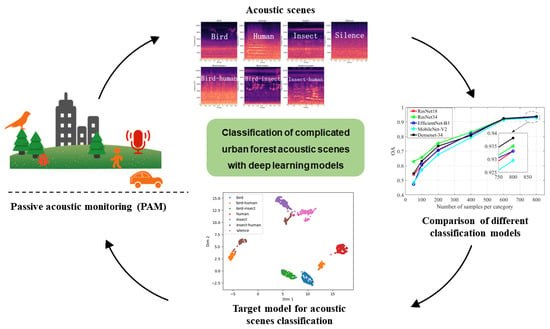
Classification of Complicated Urban Forest Acoustic Scenes with Deep Learning Models

Abstract

The use of passive acoustic monitoring (PAM) can compensate for the shortcomings of traditional survey methods on spatial and temporal scales and achieve all-weather and wide-scale assessment and prediction of environmental dynamics. Assessing the impact of human activities on biodiversity by analyzing the characteristics of acoustic scenes in the environment is a frontier hotspot in urban forestry. However, with the accumulation of monitoring data, the selection and parameter setting of the deep learning model greatly affect the content and efficiency of sound scene classification. This study compared and evaluated the performance of different deep learning models for acoustic scene classification based on the recorded sound data from Guangzhou urban forest. There are seven categories of acoustic scenes for classification: human sound, insect sound, bird sound, bird–human sound, insect–human sound, bird–insect sound, and silence. A dataset containing seven acoustic scenes was constructed, with 1000 samples for each scene. The requirements of the deep learning models on the training data volume and training epochs in the acoustic scene classification were evaluated through several sets of comparison experiments, and it was found that the models were able to achieve satisfactory accuracy when the training sample data volume for a single category was 600 and the training epochs were 100. To evaluate the generalization performance of different models to new data, a small test dataset was constructed, and multiple trained models were used to make predictions on the test dataset. All experimental results showed that the DenseNet_BC_34 model performs best among the comparison models, with an overall accuracy of 93.81% for the seven acoustic scenes on the validation dataset. This study provides practical experience for the application of deep learning techniques in urban sound monitoring and provides new perspectives and technical support for further exploring the relationship between human activities and biodiversity.

1. Introduction

Today, the impact of human activities on biodiversity has spread to every ecosystem on Earth [1]. Assessing how urbanization affects biodiversity has been the focus of urban forestry in recent decades [2]. Urbanization is growing rapidly across the globe, but how urban sprawl affects species living in urban areas is still largely unknown [3]. Understanding the interactions between urban and natural systems to provide theories and solutions for sustainable urban development will be essential for urban forests in the coming decade [4]. Habitat destruction and invasive species can lead to a general decline in biodiversity, leading to a reduction in acoustic biodiversity [5]. It becomes increasingly important to improve our monitoring capabilities and to understand the impact of human activities on biodiversity [6]. The acoustic quality of habitats is a new aspect of environmental protection [7]. With the development of sensor technology, PAM techniques are widely used in various kinds of ecological monitoring [8]. The PAM-based acoustic monitoring has received more and more attention because it can rapidly and automatically acquire large-scale spatial-temporal data and minimize the possibility of on-site observer bias [9].

An important direction in the ecology of soundscape is to explore the distribution of sound in landscape patterns and the factors influencing it and focus on ecosystem processes and the impact of human activities on biodiversity [10,11]. The soundscape consists of biophony, geophony, and anthrophony. Krause et al. [12] defined biophony and geophony as a collection of biotic and abiotic sounds (wind, rain, thunder, etc.), respectively, while Pijanowski et al. [11] expanded the soundscape categories by proposing the category of anthrophony, defining it as sounds produced directly or indirectly by humans. Soundscape properties vary according to geographic location, vegetation composition and structure, and time [13]. Identifying acoustic scene patterns in natural landscapes is essential for understanding the impact of anthropogenic changes on biodiversity. The ecologically relevant information in sound data will be maximized by classifying various sound data collected by PAM and then studying the impact of human activities on the environment [14].

Environmental sounds include many types, such as those produced by humans, tools, animals, liquids, and objects [15,16]. Many methods in environmental sound recognition come from the field of speech recognition. Among them, classification methods such as Gaussian mixture models [17], the Hidden Markov model [18], support vector machines [19], and K-nearest Neighbor algorithm [20] are the most widely used. However, traditional machine learning algorithms cannot effectively model complex environmental sounds and have poor noise robustness. For this reason, Piczak et al. [21] and Salamon et al. [22] proposed the utilization of the powerful feature extraction and classification capabilities of convolutional neural networks for environmental sound recognition. Boddapati et al. [23] proposed the application of the image recognition networks to environmental sound recognition by converting sound signals into different spectrogram features and then inputting them into AlexNet and GoogleNet, respectively. Chi et al. [24] argued that a single spectrogram feature cannot provide enough information, and therefore proposed combining two different spectrogram features before using them for recognition. In addition, to enhance the classification ability of the models, various effective methods have been proposed, such as expanding the dataset using data augmentation [22,25], using multiple deep learning models for joint prediction [26,27], and designing more suitable deep learning models [28,29,30]. However, the sound categories used in these methods are mainly from urban public or indoor environments, and samples from urban forests are less involved, which cannot meet the needs of biodiversity and human activity studies.

With the development of deep learning, deep learning techniques have been used to study the relationship between acoustic scenes and biodiversity [31,32]. In acoustic scene ecology, deep learning techniques are more often applied in species-specific identification and target sound recognition. In the 2016 BirdCLEF challenge, deep learning models were trained to identify 999 bird sounds in different recording scenes [33]. LeBien et al. [34] trained deep learning models to identify frog species in tropical acoustic scenes. Tabak et al. [35] collected the calls of ten bat species and used deep learning models for species identification. These algorithms mentioned above are for single-species recognition, and few studies have attempted to recognize acoustic scenes with a wide range of acoustic categories. Among the existing work, Fairbrass et al. [14] constructed two classification models, CityBioNet and CityAnthroNet, to measure audible biological sounds and human sounds in complex urban environments, respectively, obtaining more accurate measurements than traditional acoustic indices. To evaluate the ability of deep learning methods to classify broadly inclusive acoustic scene and to analyze model uncertainty based on deep learning methods, Quinn et al. [36] used deep learning models based on transfer learning to identify human noise (anthropophony), wildlife vocalizations (biophony), weather phenomena (geophony), quiet periods, and microphone interference (ABGQI). They demonstrated that it was possible to quantify the vocal areas of animal activity and understand the variability of human noise in this way. However, the classification models proposed in the above studies gave less consideration to the correlation between artificial and biological sounds, especially for mixed acoustic scenes such as bird–human sounds.

Birds are vital vocal species in urban forests, and their songs are an essential indicator of information on the quality of the urban forests [37]. Sound-producing insect groups such as crickets, grasshoppers, and cicadas can also be good indicators of landscape and climate change due to their small size and variable temperature [38]. Therefore, to further investigate the correlation between animal and human sounds in acoustic scenes and to better analyze the impact of human activities on biodiversity, guided by the previous work [39], we classified acoustic scenes into human sound, insect sound, bird sound, bird–human sound, insect–human sound, bird–insect sound, and silence in this study. On this basis, we used different deep learning models to learn these acoustic scene samples and compared the classification performance of different models, and we further analyzed the requirements of different models on the amount of training data and the number of training epochs. In terms of models, since deep learning models such as ResNet, DenseNet, MobileNet, and EfficientNet are very representative and have been widely used in the field of sound recognition [25,40,41,42], we used ResNet18, ResNet34, DenseNet_BC_34, MobileNet_v2, and EfficientNet_b3 to classify the acoustic scene, respectively. The specific contributions and innovations of this paper are summarized as follows: (1) By converting the classification problem of different acoustic scenes into an image recognition problem, this study proposes the DenseNet_BC_34 model to achieve the accurate recognition of seven types of acoustic scene categories; (2) The innovative construction of an acoustic scene dataset for analyzing the correlation between human and animal sounds, containing seven types of acoustic scene data with a total of 7000 samples; (3) We analyzed and compared the classification performance of ResNet18, ResNet34, DenseNet_BC_34, MobileNet_v2, and EfficientNet_b3 models on the proposed acoustic scene categories under different training data amounts and different training epochs and explored the generalization performance of different models to new data.

2. Methods

2.1. Study Area

In this study, Song Meter SM4 acoustic recorders were used to record the sounds with obvious urban–rural gradient in the northern, central, and southern urban forests of Shimen National Forest Park (SM), Maofengshan Forest Park (MF), and Dafushan Forest Park (DF) in Guangzhou. The SM is located in an exurban area, the MF is located in a suburban area, and the DF is located in an urban area. All recording sites were located in typical southern subtropical evergreen broad-leaved forests, and dominant species include Machilus nanmu, Castanopsis fissa, Liquidambar formosana, and Acacia confusa. According to human interference factors such as functional zoning and road distribution, 3 sound collection points were set in each forest park of SM, MF, and DF, with a total of 9 sound collection points, to ensure that the sounds collected in this study are representative.

2.2. Data Acquisition and Dataset Construction

The acoustic scenes in this study were divided into seven types, including human sound, insect sound, bird sound, bird–human sound, insect–human sound, bird–insect sound, and silence. Figure 1 shows typical mel spectrograms for each acoustic scene, and the specific definitions are shown in

Table A1. Acoustic scene classification criteria.

Acoustic Scene	Criteria
Human (H)	Sound clips contain only human activity sounds.
Insect (I)	The sound clip contains only insect calls, such as cicadas.
Bird (B)	The sound clip contains only bird sounds.
Bird–Human (BH)	A mixture of human sounds and bird sounds in the sound clip.
Insect–Human (IH)	A mixture of insect sounds and human sounds in the sound clip.
Bird–Insect (BI)	A mixture of bird sounds and insect sounds in the sound clip.
Silence (S)	There are no valid sound events in the sound clip.

. After acquiring a large amount of data and setting the types of sounds, the data samples of each scene were manually selected and labeled using Adobe Audition 2020. The sampling rate of each sample was resampled to 22,050 Hz, the sampling bit rate is 16 bits, and the time duration is 3–5 s. Finally, 1000 annotated samples were selected for each acoustic scene to form the complete dataset, denoted as the development dataset. The entire development dataset was sliced into training and validation datasets in a ratio of 8:2. A test dataset was also constructed for this study, in which the sample size of human sound, insect sound, bird sound, bird–human sound, insect–human sound, bird–insect sound, and silence is 113, 100, 90, 158, 159, 100, and 100, respectively. To verify which model has better generalization ability to new samples, the data collection time for this test dataset differed from that of the development dataset. Figure 2 summarizes the methodology for this work.

2.3. Feature Extraction

Spectrograms are mainly used for audio analysis [43,44]. By converting a one-dimensional audio signal into a spectrogram, the changes in the signal spectrum over time can be better reflected. To identify acoustic scenes, the mainstream practice is to convert the one-dimensional audio signal into a mel spectrogram [45]. The mel spectrogram can better characterize the signal properties by mapping the linear frequency scale to the mel scale, which mimics human auditory characteristics. The mapping relationship between linear frequency and mel frequency is shown in Equation (1). Figure 3 compares a one-dimensional waveform diagram of a bird sound signal and its corresponding mel speech spectrogram. In this study, the number of FFT points was 1024, the frameshift was 512, and the number of mel filter groups was 128. Finally, the size of the mel spectrogram was 128 × 216.

$$\left\{\begin{array}{l}{F}_{\mathrm{mel}}(f)=1125\times \ln (1+\frac{f}{700})\\ \\ F_{mel}^{-1}(f_{mel})=700\left(e^{f_{mel}/1125}-1\right)\end{array}\right.$$

(1)

2.4. Data Augmentation

The major drawback of deep learning is the extensive amount of data to train, and getting a large number of labeled samples manually is laborious. In order to solve this problem, data augmentation [22] was used to increase the number of training samples. The data augmentation strategies used in this study include noise addition, amplitude change, time shifting, and spectrum augmentation.

Noise addition adds Gaussian white noise such that the signal-to-noise ratio is $R_{snr}$ dB, where $R_{snr}$ was randomly chosen from 3 dB to 10 dB in this study. Amplitude change multiplies the audio signal by a random amplitude factor $R_{amp}$ to reduce or increase the volume, where $R_{amp}$ was randomly chosen from −12 dB to 12 dB. Time shifting randomly divides the audio signal into two parts, which are then swapped and reconnected into a new signal. Spectrum augmentation operates on the mel spectrogram in terms of frequency masking and time masking. Frequency masking randomly selects $f_r$ consecutive mel frequency channels $[f,f+f_r]$, where $f_r$ is chosen from a uniform distribution $U(0,f^{\prime })$, and $f^{\prime }$ is the masking parameter. Time masking is similar to frequency masking while working in the temporal dimension.

2.5. Deep Learning Methods

Deep learning is a branch of machine learning that uses multiple hidden nodes and nonlinear transformations to represent complex data abstractly. In contrast, traditional machine learning algorithms are limited in their ability to model complex data without a priori knowledge [46,47]. Convolutional neural networks (CNNs) are widely used in image recognition, speech recognition, and other fields, because they can learn different scales of interrelated features from input data based on mechanisms similar to the human brain. Among all available CNN models, ResNet, EfficientNet, MobileNet, and DenseNet are very representative and have been widely used in sound recognition [25,41,42,43]; ResNet18, ResNet34, DenseNet_BC_34, MobileNet_v2, and EfficientNet_b3 were selected for performance comparison.

ResNet [48] was proposed by He et al., and by introducing Skip Connection, ResNet overcomes the problem of gradient disappearance due to the increasing depth of the model, which eventually makes it possible to design models with more layers. To test the effectiveness of this model structure, two ResNet models with different depths were selected for validation. Among them, ResNet18 contains 17 convolutional layers and 1 fully connected layer, while ResNet34 contains 33 convolutional layers and 1 fully connected layer. Compared with ResNet, DenseNet [49] uses a more aggressive dense connectivity mechanism: interconnecting all layers, and each layer accepts all the layers before it as its additional input. To reduce the model parameters as much as possible, the researchers introduced Bottleneck layers and Compression operations in the model-building process to obtain the DenseNet-BC model. The DenseNet_BC_34 model we used in this study has 33 convolutional layers and 1 fully connected layer. To build deep learning models more suitable for mobile devices, Howard et al. [50] proposed MobileNet by using depthwise separable convolutions, thus building lightweight deep learning networks. MobileNet_v2 [51] is an improvement on MobileNet, which further improves the expressiveness of the model by introducing inverted residuals and linear bottlenecks. EfficientNet was proposed by Tan et al. [52]. They found that the three main dimensions that affect the accuracy of neural networks are depth, width, and resolution. They obtained a model backbone named EfficientNet_b0 by the neural architecture search (NAS) [53] technique and then scaled the above three dimensions simultaneously based on this backbone to obtain the models b1-b7 with a stunning performance. EfficientNet_b3 was chosen for the target model of this study.

2.6. Performance Evaluation

In this study, we used five quantitative criteria. Accuracy (ACC), precision (P), recall (R) and F₁ score (F₁), and overall accuracy (OA) were applied to evaluate and compare the performance of different models, as shown in Equations (2)–(6).

$$ACC=\frac{TP+TN}{TP+TN+FP+FN}\times 100\%$$

(2)

$$P=\frac{TP}{TP+FP}\times 100\%$$

(3)

$$R=\frac{TP}{TP+FN}\times 100\%$$

(4)

$$F_1=2\times \frac{P\cdot R}{P+R}$$

(5)

$$OA=\frac{{\displaystyle \sum _{i=1}^r{x}_{ii}}}{r}\times 100\%$$

(6)

Both TP and TN denote samples that are correctly classified by the model, where TP denotes true positive samples and TN denotes true negative samples. FP is false positive, indicating the negative samples that are misclassified as positive by the model; FN is false negative, indicating the positive samples that are misclassified as negative by the model. Accuracy is considered from the perspective of the total training samples, indicating the number of correctly predicted samples as a percentage of the total number of samples. Precision represents the ratio of the number of correctly predicted positive samples to the number of all predicted positive samples, while the ratio of the number of samples predicted to be positive and actually positive to the number of all positive samples is called recall. Accuracy and recall are metrics for evaluating model performance, but there is a trade-off between them [54]. As a reconciled average of accuracy and recall, the F₁ score is often used as an overall metric. In addition, r denotes the number of samples in the validation set, and x_ii denotes the value of the element in the ith row and ith column of the confusion matrix. In all subsequent experiments, the experimental results were calculated as the average of three replicate experiments.

2.7. Experimental Environmant

The learning environment for both CNN models was a computer with a Windows operating system (Windows 10, Professional, Version-22H2), Inter Core (TM) i7-1107F central processing unit, and NVIDIA Geforce RTX 2080 Super GPU. Cuda 11.1 and cnDNN 11.2 were used to support the GPU with deep learning. All CNN models were modeled using the Python tool in the Pytorch framework. Matplotlib (Matplotlib: v3.6.2 library by J. D. Hunter, https://doi.org/10.5281/zenodo.7275322, accessed on 3 November 2022) and Librosa (Librosa: v0.9.2 library by B. McFee et al., https://doi.org/10.5281/zenodo.6759664, accessed on 27 June 2022) were used to export figures, load audio files, and calculate the mel spectrogram.

3. Results

3.1. Comparison of the Results of Different Models with Different Amounts of Training Data

This section analyzes the classification results of different models for the same validation dataset under the maximum training epochs (200 epochs) with different training sample amounts (the sample amounts here refer to the number of training samples for a single class).

As shown in

Table 1. The results of different models with different amounts of training data.

Model	OA (%)
	50 1	100 1	200 1	400 1	600 1	800 1
ResNet18	53.86	60.33	70.95	81.71	91.79	93.31
ResNet34	62.90	65.79	75.31	83.02	92.12	93.50
EfficientNet_b3	47.40	61.00	70.57	81.76	92.28	93.31
MobileNet_v2	48.33	57.19	67.64	79.31	91.48	92.95
DenseNet_BC_34	54.69	63.21	73.50	80.71	92.40	93.81

¹ represents the number of training samples for each acoustic scene. The highest OA of the model with the same number of training samples is marked in bold.

, the DenseNet_BC_34 model achieved the highest overall accuracy when the number of training samples was greater than or equal to 600 compared with other models. For example, the overall accuracy of the DenseNet_BC_34 model was 92.40% and 93.81% at training sample numbers of 600 and 800, respectively. The ResNet34 model achieved the highest overall accuracy with 62.90%, 65.79%, 75.31%, and 83.02% for training sample numbers of 50, 100, 200, and 400, respectively.

With the increase in training samples, the accuracy of each model improved accordingly. When the number of training samples increased from 50 to 100, the maximum improved accuracy of different model was 13.60% and the minimum improved accuracy was 2.89%; When the number of training samples increased from 100 to 200, the maximum improved accuracy of different model was 10.62% and the minimum improved accuracy was 9.52%; When the number of training samples increased from 200 to 400, the maximum improved accuracy of different model was 11.67% and the minimum improved accuracy was 7.21%; When the number of training samples increased from 400 to 600, the maximum improved accuracy of different model was 12.17% and the minimum improved accuracy was 9.1%; When the number of training samples increased from 600 to 800, the maximum improved accuracy of different model was 1.52% and the minimum improved accuracy was 1.03%.

Figure 4 is a visualization of Table 1, clearly showing the trend of the overall accuracy of each deep learning model after the size of training samples increases. When the number of training samples was less than 600, the overall accuracy of each model changed significantly; when the number of training samples was greater than or equal to 600, the increase in the number of training samples contributed little to the overall accuracy improvement of each model.

3.2. Effect of Training Epochs on Model Classification Results

In this study, the number of training epochs was increased by 50, and the overall accuracy was evaluated for 50, 100, 150, and 200 training epochs (the OA in

Table 2. The overall accuracy of the different models with different training epochs.

Model	Epoch	OA (%)
		50 1	100 1	200 1	400 1	600 1	800 1
ResNet18	50 2	51.88	59.35	69.52	81.07	91.50	92.83
	100 2	53.64 (+1.76)	59.95 (+0.60)	70.95 (+1.43)	81.71 (+0.64)	91.64 (+0.14)	93.31 (+0.48)
	150 2	53.86 (+0.21)	59.95 (+0.00)	70.95 (+0.00)	81.71 (+0.00)	91.64 (+0.00)	93.31 (+0.00)
	200 2	53.86 (+0.00)	60.33 (+0.38)	70.95 (+0.00)	81.71 (+0.00)	91.79 (+0.15)	93.31 (+0.00)
ResNet34	50 2	58.50	64.29	75.17	82.72	91.55	92.76
	100 2	62.90 (+4.40)	64.29 (+0.00)	75.31 (+0.14)	83.02 (+0.31)	92.12 (+0.57)	93.50 (+0.74)
	150 2	62.90 (+0.00)	65.79 (+1.50)	75.31 (+0.00)	83.02 (+0.00)	92.12 (+0.00)	93.50 (+0.00)
	200 2	62.90 (+0.00)	65.79 (+0.00)	75.31 (+0.00)	83.02 (+0.00)	92.12 (+0.00)	93.50 (+0.00)
EfficientNet_b3	50 2	36.31	52.83	67.69	80.26	91.50	92.97
	100 2	44.55 (+8.24)	56.93 (+4.10)	69.05 (+1.36)	81.31 (+1.05)	92.28 (+0.78)	93.21 (+0.24)
	150 2	47.40 (+2.85)	58.62 (+1.69)	69.47 (+0.43)	81.47 (+0.16)	92.28 (+0.00)	93.21 (+0.00)
	200 2	47.40 (+0.00)	61.00 (+2.38)	70.57 (+1.10)	81.76 (+0.29)	92.28 (+0.00)	93.31 (+0.10)
MobileNet_v2	50 2	41.62	50.59	63.17	76.12	90.45	92.36
	100 2	44.86 (+3.24)	53.15 (+2.55)	64.81 (+1.64)	78.90 (+2.78)	91.36 (+0.91)	92.79 (+0.43)
	150 2	47.67 (+2.81)	55.24 (+2.09)	66.93 (+2.12)	79.19 (+0.29)	91.48 (+0.12)	92.95 (+0.17)
	200 2	48.33 (+0.67)	57.19 (+1.95)	67.64 (+0.72)	79.31 (+0.12)	91.48 (+0.00)	92.95 (+0.00)
DensNet_BC_34	50 2	49.24	56.59	69.69	78.41	90.62	91.79
	100 2	52.05 (+2.81)	60.57 (+3.98)	72.88 (+3.19)	80.67 (+2.26)	91.78 (+1.17)	92.86 (+1.07)
	150 2	53.12 (+1.07)	63.21 (+2.64)	73.41 (+0.52)	80.71 (+0.05)	92.19 (+0.41)	93.64 (+0.79)
	200 2	54.69 (+1.57)	63.21 (+0.00)	73.50 (+0.09)	80.71 (+0.00)	92.40 (+0.21)	93.81 (+0.16)

¹ represents the number of training samples for each acoustic scene. ² Epoch. Bolded numbers represent the maximum value.

represents the highest overall accuracy obtained by the model up to the current training epoch). Table 2 shows the effect of training epochs on the overall accuracy of different deep learning models with varying numbers of training samples.

As can be seen from Table 2, for different numbers of training samples, the overall accuracy of most models improved somewhat with increasing training epochs. However, the accuracy of some models stopped growing after 100 training epochs. For example, in ResNet34, when the training data amount was greater than or equal to 200, the overall accuracy did not increase after 100 epochs, which was 0.0%; in ResNet18, when the training data amount was 200, 400, and 800, respectively, the overall accuracy also did not increase after 100 epochs of training.

By analyzing, it can be found that for almost all different amounts of training data, all tested models have the largest increase in overall accuracy after increasing the training epochs from 50 to 100. As an exception, ResNet34 had the largest overall accuracy growth after increasing the training epochs from 100 to 150 at a training data volume of 100, while MobileNet_V2 had the largest overall accuracy growth after raising the training epochs from 100 to 150 at a training data volume of 200.

Figure 5 shows the visualization of Table 2, from which we can see more clearly the trend of the overall accuracy as the number of training epochs increases.

3.3. Comparison of Different Models’ Ability to Predict New Data

This section analyzes the classification accuracy of different models for new data by predicting samples from the test dataset to evaluate the generalization ability of different models for new data. Models used in this section have been trained using the entire training dataset.

As can be seen from

Table 3. Overall accuracy of different models on the test dataset.

Model	OA (%)
ResNet18	70.69
ResNet34	69.47
EfficientNet_B3	65.65
MobileNet_V2	61.18
DenseNet_BC_34	73.50

Bolded numbers represent the maximum value.

, the DenseNet_BC_34 model had the highest overall accuracy of 73.50% for the test dataset, which exceeded the second highest model, ResNet18, by 2.81%. The model with the lowest overall accuracy was MobileNet_V2, which had an overall accuracy of 61.18% for the test dataset.

3.4. Analysis Results of Acoustic Scene Classification Using the DenseNet_BC_34 Mode

The DenseNet_BC_34 model was evaluated for acoustic scene classification using the validation dataset in this section. This model was chosen because it mostly achieved the best results when trained with different numbers of training samples (see Table 1) and had a relatively low number of model parameters and floating-point operations (see

Table A2. FLOPs and Params of different models.

Model	FLOPs (G)	Params (M)
ResNet18	15.01	11.17
ResNet34	31.14	21.28
EfficientNet_b3	0.01	10.72
MobileNet_v2	0.18	2.23
DenseNet_BC_34	0.40	0.12

Minimum values are shown in bold.

). It also had the best generalization capability for new data (see Table 3). Figure 6 shows the confusion matrix of the DenseNet_BC_34 model on the validation dataset.

Table 4. Quantitative analysis results of the DenseNet_BC_34 model.

Class	TP	TN	FP	FN	ACC (%)	P (%)	R (%)	F1 (%)
B	191	1182	18	9	98.07	91.39	95.50	93.40
BH	172	1189	11	28	97.21	93.99	86.00	89.82
BI	189	1190	10	11	98.50	94.97	94.50	94.74
H	189	1179	21	11	97.71	90.00	94.50	92.20
I	190	1190	10	10	98.57	95.00	95.00	95.00
IH	188	1190	10	12	98.43	94.95	94.00	94.47
S	195	1192	8	5	99.07	96.06	97.50	96.77

shows the quantitative analysis results when testing the validation dataset using the DenseNet_BC_34 model. As shown in Table 4, the DenseNet_BC_34 model had a strong classification capability for acoustic scenes. From the results of individual categories, the accuracy (ACC) of each acoustic scene exceeded 97.00%, the precision (P) was higher than 90.00%, and the recall (R) was greater than or equal to 94.00%, except for BH, and the F₁ score of each scene was higher than 89%. For example, the accuracy, precision, recall, and F₁ scores for B were 98.07%, 91.39%, 95.50%, and 93.40%, respectively. The classification results of the DenseNet_BC_34 model for each scene showed that the model could effectively identify each acoustic scene sample from the validation dataset.

In addition, the results in Table 4 also show that the DenseNet_BC_34 model had some misclassification results when classifying acoustic scene samples. For example, the FPs of categories B, BH, BI, H, I, IH, and S were 18, 11, 10, 21, 10, 10, and 8, respectively, while the FNs were 9, 28, 11, 11, 10, 12, and 5, respectively. Figure 7 shows the visualization of the embedding features of the validation dataset. As shown in Figure 7, some of the features are closer together in the feature space, which is a possible cause of misclassification.

4. Discussion

This study used deep-learning-based acoustic scene classification algorithms to build a framework that can analyze large amounts of audio data automatically, which can be an effective tool for researchers to study the relationship between urban biodiversity and human activities. Using reliable automated analysis tools can significantly reduce time and labor costs and better prevent the introduction of human error factors.

4.1. Effect of Training Data Amount and Epochs on Model Classification Performance

The minimum amount of data and the minimum number of epochs for deep learning training are vital to the workload and efficiency of researchers. In terms of training data amount, we calculated the overall accuracy for different models with training data amounts of 50, 100, 200, 400, 600, and 800, respectively. The results showed that the overall accuracy of all models improved as the number of data increased. When the training data amount increased from 400 to 600, the overall accuracy of the five models increased the most on average, by 10.71%. When the training data amount was greater than 600, the overall accuracy of the models had the lowest increase. For example, after the sample size increased from 600 to 800, the average growth of the overall accuracy of the five models was only 1.36%. By analyzing the result, we believe that 600 training samples per category are sufficient for the number of sound samples required in this study. The overall accuracy of all tested models on the validation dataset had exceeded 92% at a data volume of 600 training samples per category, and adding more samples had little benefit on the improvement of model accuracy after exceeding 600 samples. On the one hand, although deep learning is a data-driven approach, more training data can lead to better model capabilities [55]; on the other hand, related studies also point out that when the classification accuracy improvement is small, researchers should make cost considerations to justify the effort of collecting more data and performing labeling [56].

Although the overall accuracy of most of the models showed an increasing trend as the number of training epochs increased, it showed little improvement after 100 training epochs. The overall accuracy stabilized at a low level with a small amount of training sample data, which indicates that the models were unable to learn more information with insufficient data, which needs to be changed by increasing the amount of training data rather than simply increasing the number of training rounds.

4.2. DenseNet_BC_34 Model for Classification of the Acoustic Scenes

The DenseNet_BC_34 model has certain advantages over other models. Firstly, the model can achieve an overall accuracy of 92.40% and 93.81% among all models with a training sample size of 600 and 800, respectively; secondly, there are also significant differences between the floating-point operations and the number of training parameters of the five tested models. Table A2 shows that both ResNet18 and ResNet34 have much larger floating-point operations than the other models, while the remaining three are relatively small in this respect. DenseNet_BC_34 has the smallest number of parameters among the remaining three models, which is only 0.12 M. In addition, as shown in Section 3.3, the DenseNet _BC_34 model also had the best predictive performance for new data in the test dataset among all models. Therefore, the DenseNet _BC_34 model is superior to other models in this study.

The DenseNet_BC_34 model obtained after training on the complete training dataset had an overall accuracy of 93.81%. The quantitative analysis of the seven categories of data in the validation dataset, as seen in Table 4, shows that the ACC of each acoustic scene was above 97.00%, which indicates that the model can distinguish each of our predefined acoustic scenes well. It is very capable in the ecological acoustic scene classification task. The classification process will inevitably result in some misclassified samples. As seen from the confusion matrix in Figure 6, the misclassification occurred mainly between BH and H, BH and B, and BI and B. These are misclassifications that occurred between mixed sound types and single sound types. The analysis of the misclassified samples revealed that the main reason for the misclassifications was the relatively low sound intensity of a specific category in the mixed sound samples, which the model could not recognize. It is common in reality, where the intensity between different types of sounds may differ significantly due to the distance, making it more difficult to identify samples of mixed categories of sounds. We extracted embedding features from the samples of the validation dataset and used the UMAP algorithm [57] to reduce their dimensionality and visualize them, as shown in Figure 7, from which we can see that there is a high degree of similarity between some of the categories.

Considering that the models will be used to predict the environmental sound data acquired at different periods after the models are trained, a test dataset was specifically set up in which the data were obtained at different times from those in the development dataset, to evaluate the generalizability of different models to new data. As shown in Table 3, we can see that the DenseNet_BC_34 model had the best generalizability for new data, with an overall accuracy of 73.50%, which was somewhat attenuated compared to the overall accuracy of 93.81% achieved on the validation dataset. The reason may be that the same acoustic scene contains a variety of sound patterns, and the patterns in the test dataset have not yet been learned during the model training process and ultimately cannot be recognized by the model. This result instructs the researchers concerned that in the process of constructing training datasets for the same category of an acoustic scene, they also need to collect as many samples with different sound patterns as possible to enrich the sound patterns that can be learned during the model training and eventually improve the classification ability of the model for new data.

4.3. Comparison of Related Studies

In contrast to other related studies, for example, Mullet et al. [58] used a machine-learning-based stochastic gradient boosting method to analyze three categories of acoustic scenes and investigated the relationship between different acoustic scene components over time and space in winter. In Mullet et al.’s study, they manually identified and labeled nearly 60,000 sound samples, which is a very labor-intensive task, while our proposed method requires less than 5000 sound samples to be labeled (600 samples per acoustic scene), requiring only a small amount of manual labeling cost. In the study by Quinn et al. [36], they classified sound categories into five types: anthropophony, biophony, geophony, quiet periods, and microphone interference. They trained the data using a pre-trained MobileNet_v2 model based on transfer learning. To increase the number of training samples, they also used the Freesound dataset [59] as auxiliary data added to the training process. However, in our study, all data came from real samples of actual scenes, which can make the model fit the real scenes to a certain extent. Quinn et al. [36] used a transfer-learning-based method to reduce the training time of the model, which is a worthwhile practice. In addition, in terms of acoustic scene categories, both of these studies only classified broadly inclusive acoustic scenes such as geophony or biophony. In contrast, our study made a distinction between mixed sound types such as BH and IH, which will help further analyze which birds or insects are more likely to coexist with humans. In the study of other animal populations, Dufourq et al. [60] designed and trained a high-accuracy deep learning model for detecting the call of Hainan gibbon Nomascus hainanus in the massive data collected by PAM. In this way, the efficiency of wildlife conservation can be improved, but how to obtain enough call samples of the target species is also a problem (for example, the habitat may be inaccessible, or the population may be reduced because the species is threatened).

5. Conclusions

In urban forest research, analyzing acoustic scenes in the environment to assess how human activities impact biodiversity is a frontier hotspot. However, the knowledge barriers of deep learning algorithms such as the accumulation of monitoring data and the selection and parameter setting of the deep learning model greatly limit the application of acoustic technologies in urban forestry. We validate the feasibility of acoustic scene classification techniques in the urban forest domain in terms of model selection, number of learning samples, and number of iterations, respectively, to help researchers who wish to use acoustic methods to solve ecological problems to quickly find suitable deep learning models and methods for themselves. In this study, we compared the ability of different models to recognize biological acoustic scenes based on deep learning techniques and proposed that DenseNet_BC_34 is relatively better among the five models. Based on this, the DenseNet_BC_34 model was used to classify seven acoustic scenes and analyze the classification results. We compared the performance of different models under different amounts of training data, tested the ability of different models to classify new data, and finally gave suggestions for dataset construction.

With the development of deep learning and sound recognition technology, recognizing and classifying acoustic scenes based on deep learning will be more closely integrated with urban forestry. We believe that PAM with an automatic data upload function can be developed to upload the sound data collected in the field directly to the cloud platform and use deep learning models to automatically perform sound detection and classification, which will significantly reduce the labor cost. In addition, the deep-learning-based approach can also track the relationship of acoustic scenes over time and space in real time, providing valuable clues for related biodiversity conservation efforts.

References

1. Masood, E. Battle over biodiversity. Nature 2018, 560, 423–425. [Google Scholar] [CrossRef] [Green Version]
2. Wu, J. Urban ecology and sustainability: The state-of-the-science and future directions. Landsc. Urban Plan. 2014, 125, 209–221. [Google Scholar] [CrossRef]
3. Rivkin, L.R.; Santangelo, J.S.; Alberti, M.; Aronson, M.F.J.; De Keyzer, C.W.; Diamond, S.E.; Fortin, M.; Frazee, L.J.; Gorton, A.J.; Hendry, A.P.; et al. A roadmap for urban evolutionary ecology. Evol. Appl. 2019, 12, 384–398. [Google Scholar] [CrossRef] [Green Version]
4. Yang, J. Big data and the future of urban ecology: From the concept to results. Sci. China Earth Sci. 2020, 63, 1443–1456. [Google Scholar] [CrossRef]
5. Farina, A.; Pieretti, N.; Malavasi, R. Patterns and dynamics of (bird) soundscapes: A biosemiotic interpretation. Semiotica 2014, 2014, 109. [Google Scholar] [CrossRef]
6. Hampton, S.E.; Strasser, C.A.; Tewksbury, J.J.; Gram, W.K.; Budden, A.E.; Batcheller, A.L.; Duke, C.S.; Porter, J.H. Big data and the future of ecology. Front. Ecol. Environ. 2013, 11, 156–162. [Google Scholar] [CrossRef] [Green Version]
7. Dumyahn, S.L.; Pijanowski, B.C. Soundscape conservation. Landsc. Ecol. 2011, 26, 1327–1344. [Google Scholar] [CrossRef]
8. Hou, Y.; Yu, X.; Yang, J.; Ouyang, X.; Fan, D. Acoustic Sensor-Based Soundscape Analysis and Acoustic Assessment of Bird Species Richness in Shennongjia National Park, China. Sensors 2022, 22, 4117. [Google Scholar] [CrossRef]
9. Sugai, L.S.M.; Silva, T.S.F.; Ribeiro, J.W.; Llusia, D. Terrestrial Passive Acoustic Monitoring: Review and Perspectives. Bioscience 2019, 69, 15–25. [Google Scholar] [CrossRef]
10. Kasten, E.P.; Gage, S.H.; Fox, J.; Joo, W. The remote environmental assessment laboratory’s acoustic library: An archive for studying soundscape ecology. Ecol. Inform. 2012, 12, 50–67. [Google Scholar] [CrossRef]
11. Pijanowski, B.C.; Villanueva-Rivera, L.J.; Dumyahn, S.L.; Farina, A.; Krause, B.L.; Napoletano, B.M.; Gage, S.H.; Pieretti, N. Soundscape Ecology: The Science of Sound in the Landscape. Bioscience 2011, 61, 203–216. [Google Scholar] [CrossRef] [Green Version]
12. Krause, B. Bioacoustics: Habitat Ambience & Ecological Balance. Whole Earth Rev. 1987, 57. [Google Scholar]
13. Sueur, J.; Krause, B.; Farina, A. Acoustic biodiversity. Curr. Biol. 2021, 31, R1172–R1173. [Google Scholar] [CrossRef]
14. Fairbrass, A.J.; Firman, M.; Williams, C.; Brostow, G.; Titheridgem, H.; Jones, K.E. CityNet-Deep learning tools for urban ecoacoustic assessment. Methods Ecol. Evol. 2019, 10, 186–197. [Google Scholar] [CrossRef] [Green Version]
15. Lewis, J.W.; Wightman, F.L.; Brefczynski, J.A.; Phinney, R.E.; Binder, J.R.; DeYoe, E.A. Human Brain Regions Involved in Recognizing Environmental Sounds. Cereb. Cortex 2004, 14, 1008–1021. [Google Scholar] [CrossRef] [Green Version]
16. Alluri, V.; Kadiri, S.R. Neural Correlates of Timbre Processing, in Timbre: Acoustics, Perception, and Cognition; Springer: Berlin/Heidelberg, Germany, 2019; pp. 151–172. [Google Scholar]
17. Eronen, A.; Tuomi, J.; Klapuri, A.; Fagerlund, S.; Sorsa, T.; Lorho, G.; Huopaniemi, J. Audio-based context awareness acoustic modeling and perceptual evaluation. In Proceedings of the 2003 IEEE International Conference on Acoustics, Speech, and Signal Processing, New Platz, NY, USA, 6–10 April 2003. [Google Scholar]
18. Eronen, A.J.; Peltonen, V.T.; Tuomi, J.; Klapuri, A.; Fagerlund, S.; Sorsa, T.; Lorho, G.; Huopaniemi, J. Audio-based context recognition. IEEE Trans. Audio Speech Lang. Process. 2006, 14, 321–329. [Google Scholar] [CrossRef]
19. Lei, B.Y.; Mak, M.W. Sound-Event Partitioning and Feature Normalization for Robust Sound-Event Detection. In Proceedings of the 19th International Conference on Digital Signal Processing (DSP), Hong Kong, China, 20–23 August 2014. [Google Scholar]
20. Chu, S.; Narayanan, S.; Kuo, C.C.J. Environmental Sound Recognition with Time-Frequency Audio Features. IEEE Trans. Audio Speech Lang. Process. 2009, 17, 1142–1158. [Google Scholar] [CrossRef]
21. Piczak, K.J. Environmental sound classification with convolutional neural networks. In Proceedings of the IEEE International Workshop on Machine Learning for Signal Processing, Boston, MA, USA, 17–20 September 2015. [Google Scholar]
22. Salamon, J.; Bello, J.P. Deep Convolutional Neural Networks and Data Augmentation for Environmental Sound Classification. IEEE Signal Process. Lett. 2017, 24, 279–283. [Google Scholar] [CrossRef]
23. Boddapati, V.; Petef, A.; Rasmusson, J.; Lundberg, L. Classifying environmental sounds using image recognition networks. In Proceedings of the 21st International Conference on Knowledge—Based and Intelligent Information and Engineering Systems (KES), Aix Marseille University, St. Charles Campus, Marseille, France, 6–8 September 2017. [Google Scholar]
24. Chi, Z.; Li, Y.; Chen, C. Deep Convolutional Neural Network Combined with Concatenated Spectrogram for Environmental Sound Classification. In Proceedings of the 2019 IEEE 7th International Conference on Computer Science and Network Technology (ICCSNT), Dalian, China, 19–20 October 2019. [Google Scholar]
25. Mushtaq, Z.; Su, S.-F.; Tran, Q.-V. Spectral images based environmental sound classification using CNN with meaningful data augmentation. Appl. Acoust. 2021, 172, 107581. [Google Scholar] [CrossRef]
26. Qiao, T.; Zhang, S.; Cao, S.; Xu, S. High Accurate Environmental Sound Classification: Sub-Spectrogram Segmentation versus Temporal-Frequency Attention Mechanism. Sensors 2021, 21, 5500. [Google Scholar] [CrossRef] [PubMed]
27. Li, R.; Yin, B.; Cui, Y.; Li, K.; Du, Z. Research on Environmental Sound Classification Algorithm Based on Multi-feature Fusion. In Proceedings of the IEEE 9th Joint International Information Technology and Artificial Intelligence Conference (ITAIC), Chongqing, China, 11–20 December 2020. [Google Scholar]
28. Wu, B.; Zhang, X.-P. Environmental Sound Classification via Time–Frequency Attention and Framewise Self-Attention-Based Deep Neural Networks. IEEE Internet Things J. 2022, 9, 3416–3428. [Google Scholar] [CrossRef]
29. Song, H.; Deng, S.; Han, J. Exploring Inter-Node Relations in CNNs for Environmental Sound Classification. IEEE Signal Process. Lett. 2022, 29, 154–158. [Google Scholar] [CrossRef]
30. Tripathi, A.M.; Mishra, A. Environment sound classification using an attention-based residual neural network. Neurocomputing 2021, 460, 409–423. [Google Scholar] [CrossRef]
31. Lin, T.; Tsao, Y. Source separation in ecoacoustics: A roadmap towards versatile soundscape information retrieval. Remote. Sens. Ecol. Conserv. 2020, 6, 236–247. [Google Scholar] [CrossRef] [Green Version]
32. Sethi, S.S.; Jones, N.S.; Fulcher, B.D.; Picinali, L.; Clink, D.J.; Klinck, H.; Orme, C.D.L.; Wrege, P.H.; Ewers, R.M. Characterizing soundscapes across diverse ecosystems using a universal acoustic feature set. Proc. Natl. Acad. Sci. USA 2020, 117, 17049–17055. [Google Scholar] [CrossRef]
33. Goëau, H.; Glotin, H.; Joly, A.; Vellinga, W.; Planqué, R. LifeCLEF Bird Identification Task 2016: The arrival of Deep learning. Comput. Sci. 2016, 2016, 6569338. [Google Scholar]
34. LeBien, J.; Zhong, M.; Campos-Cerqueira, M.; Velev, J.P.; Dodhia, R.; Ferres, J.L.; Aide, T.M. A pipeline for identification of bird and frog species in tropical soundscape recordings using a convolutional neural network. Ecol. Inform. 2020, 59, 101113. [Google Scholar] [CrossRef]
35. Tabak, M.A.; Murray, K.L.; Reed, A.M.; Lombardi, J.A.; Bay, K.J. Automated classification of bat echolocation call recordings with artificial intelligence. Ecol. Inform. 2022, 68, 101526. [Google Scholar] [CrossRef]
36. Quinn, C.A.; Burns, P.; Gill, G.; Baligar, S.; Snyder, R.L.; Salas, L.; Goetz, S.J.; Clark, M.L. Soundscape classification with convolutional neural networks reveals temporal and geographic patterns in ecoacoustic data. Ecol. Indic. 2022, 138, 108831. [Google Scholar] [CrossRef]
37. Hong, X.-C.; Wang, G.-Y.; Liu, J.; Song, L.; Wu, E.T. Modeling the impact of soundscape drivers on perceived birdsongs in urban forests. J. Clean. Prod. 2020, 292, 125315. [Google Scholar] [CrossRef]
38. Schmidt, A.K.D.; Balakrishnan, R. Ecology of acoustic signaling and the problem of masking interference in insects. J. Comp. Physiol. A Neuroethol. Sens. Neural Behav. Physiol. 2015, 201, 133–142. [Google Scholar] [CrossRef] [PubMed]
39. Hao, Z.; Zhan, H.; Zhang, C.; Pei, N.; Sun, B.; He, J.; Wu, R.; Xu, X.; Wang, C. Assessing the effect of human activities on biophony in urban forests using an automated acoustic scene classification model. Ecol. Indic. 2022, 144, 109437. [Google Scholar] [CrossRef]
40. Ul Haq, H.F.D.; Ismail, R.; Ismail, S.; Purnama, S.R.; Warsito, B.; Setiawan, J.D.; Wibowo, A. EfficientNet Optimization on Heartbeats Sound Classification. In Proceedings of the 5th International Conference on Informatics and Computational Sciences (ICICoS), Aachen, Germany, 24–25 November 2021. [Google Scholar]
41. Xu, J.X.; Lin, T.-C.; Yu, T.-C.; Tai, T.-C.; Chang, P.-C. Acoustic Scene Classification Using Reduced MobileNet Architecture. In Proceedings of the 20th IEEE International Symposium on Multimedia (ISM), Taichung, Taiwan, 10–12 December 2018. [Google Scholar]
42. Mushtaq, Z.; Su, S.-F. Efficient Classification of Environmental Sounds through Multiple Features Aggregation and Data Enhancement Techniques for Spectrogram Images. Symmetry 2020, 12, 1822. [Google Scholar] [CrossRef]
43. Briggs, F.; Lakshminarayanan, B.; Neal, L.; Fern, X.Z.; Raich, R.; Hadley, S.J.K.; Hadley, A.S.; Betts, M.G. Acoustic classification of multiple simultaneous bird species: A multi-instance multi-label approach. J. Acoust. Soc. Am. 2012, 131, 4640–4650. [Google Scholar] [CrossRef] [Green Version]
44. Strout, J.; Rogan, B.; Seyednezhad, S.M.; Smart, K.; Bush, M.; Ribeiro, E. Anuran call classification with deep learning. In Proceedings of the IEEE International Conference on Acoustics, Speech, and Signal Processing (ICASSP), New Orleans, LA, USA, 5–7 March 2017. [Google Scholar]
45. Rabiner, L.; Schafer, R. Theory and Applications of Digital Speech Processing; Universidad Autónoma de Madrid: Madrid, Spain, 2011. [Google Scholar]
46. Christin, S.; Hervet, É.; LeComte, N. Applications for deep learning in ecology. Methods Ecol. Evol. 2019, 10, 1632–1644. [Google Scholar] [CrossRef]
47. LeCun, Y.; Bengio, Y.; Hinton, G. Deep learning. Nature 2015, 521, 436–444. [Google Scholar] [CrossRef] [PubMed]
48. He, K.M.; Zhang, X.; Ren, S.; Sun, J. Deep Residual Learning for Image Recognition. In Proceedings of the 2016 IEEE Conference on Computer Vision and Pattern Recognition (CVPR), Seattle, WA, USA, 27–30 June 2016. [Google Scholar]
49. Huang, G.; Liu, Z.; Van Deer Maaten, L.; Weinberger, K.Q. Densely Connected Convolutional Networks. In Proceedings of the 30th IEEE/CVF Conference on Computer Vision and Pattern Recognition (CVPR), Honolulu, HI, USA, 21–26 July 2017. [Google Scholar]
50. Howard, A.G.; Zhu, M.; Chen, B.; Kalenichenko, D.; Wang, W.; Weyand, T.; Andreetto, M.; Adam, H. MobileNets: Efficient Convolutional Neural Networks for Mobile Vision Applications. arXiv 2017, arXiv:1704.04861. [Google Scholar]
51. Sandler, M.; Howard, A.G.; Zhu, M.; Zhmoginov, A.; Chen, L.-C. MobileNetV2: Inverted Residuals and Linear Bottlenecks. In Proceedings of the 31st IEEE/CVF Conference on Computer Vision and Pattern Recognition (CVPR), Salt Lake City, UT, USA, 18–23 June 2018. [Google Scholar]
52. Tan, M.X.; Le, Q.V. EfficientNet: Rethinking Model Scaling for Convolutional Neural Networks. In Proceedings of the 36th International Conference on Machine Learning (ICML), Long Beach, CA, USA, 10–15 June 2019. [Google Scholar]
53. Tan, M.X.; Chen, B.; Pang, R.; Vasudevan, V.; Sandler, M.; Howard, A.; Quoc, V.L. MnasNet: Platform-Aware Neural Architecture Search for Mobile. In Proceedings of the 32nd IEEE/CVF Conference on Computer Vision and Pattern Recognition (CVPR), Long Beach, CA, 16–20 June 2019. [Google Scholar]
54. Witten, I.H.; Frank, E. Data Mining: Practical Machine Learning Tools and Techniques, 3rd ed.; Elsevier: Amsterdam, The Netherlands, 2005. [Google Scholar]
55. Stowell, D. Computational bioacoustics with deep learning: A review and roadmap. Peerj 2022, 10, 13152. [Google Scholar] [CrossRef]
56. Thian, Y.L.; Ng, D.W.; Hallinan, J.T.P.D.; Jagmohan, P.; Sia, S.Y.; Mohamed, J.S.A.; Quek, S.T.; Feng, M. Effect of Training Data Volume on Performance of Convolutional Neural Network Pneumothorax Classifiers. J. Digit. Imaging 2021, 35, 881–892. [Google Scholar] [CrossRef]
57. Mcinnes, L.; Healy, J. UMAP: Uniform Manifold Approximation and Projection for Dimension Reduction. J. Open Source Softw. 2018, 3, 861. [Google Scholar] [CrossRef]
58. Mullet, T.C.; Gage, S.H.; Morton, J.M.; Huettmann, F. Temporal and spatial variation of a winter soundscape in south-central Alaska. Landsc. Ecol. 2016, 31, 1117–1137. [Google Scholar] [CrossRef]
59. Font, F.; Roma, G.; Serra, X. Freesound technical demo. ACM 2013, 2013, 411–412. [Google Scholar]
60. Dufourq, E.; Durbach, I.; Hansford, J.P.; Hoepfner, A.; Ma, H.; Bryant, J.V.; Stender, C.S.; Li, W.; Liu, Z.; Chen, Q.; et al. Automated detection of Hainan gibbon calls for passive acoustic monitoring. Remote. Sens. Ecol. Conserv. 2021, 7, 475–487. [Google Scholar] [CrossRef]
Figure 1. Mel spectrograms for different acoustic scenes.
Forests 14 00206 g001
Figure 2. Dataset construction.
Forests 14 00206 g002
Figure 3. Waveforms of bird calls and the corresponding mel spectrogram.
Forests 14 00206 g003
Figure 4. The trend of the overall accuracy of different models with the change of training samples.
Forests 14 00206 g004
Figure 5. Trend of the overall accuracy of the model with different training epochs.
Forests 14 00206 g005
Figure 6. Confusion matrix for DenseNet_BC_34.
Forests 14 00206 g006
Figure 7. Visualization of the embedding features of the validation dataset.
Forests 14 00206 g007