Abstract
Understanding the spatial and temporal variations of urban carbon dioxide fluxes () and their influencing factors is crucial for solving urban climate problems and promoting the development of low-carbon cities. In this study, the carbon dioxide flux () in Changsha City, China, was analyzed using the eddy covariance technique and flux footprint model. The results showed that the extent of the flux footprint within the observation site was mostly limited to 500 m. Diurnal variation of showed a regular pattern influenced by plant photosynthesis and traffic flow. Meanwhile, photosynthesis was directly regulated by photosynthetically active radiation and indirectly regulated by air temperature and water vapor pressure differences. The average value of was lower during the daytime than at night, indicating the high vegetation cover (43.5%) in the study area. In addition, there were spatial characteristics of in each wind direction due to different surface land use in the study area. Notably, a decreasing trend in carbon dioxide content was observed after the area covered by vegetation was 1.8 times the area of buildings and major roads combined. These findings guide climate management, urban planning, and sustainable development toward a low-carbon society.
1. Introduction
Urban areas contribute to approximately 70%~80% of global carbon emissions even though they cover only approximately 2% of the Earth’s land surface, exerting significant and far-reaching impacts on global carbon cycling and climate change [1,2,3]. The undeniable reality of global warming has emphasized the importance of conducting thorough research on carbon cycling processes and their underlying mechanisms in urban ecosystems [4,5,6]. However, the highly heterogeneous and complex distribution of carbon sources and sinks in urban land surfaces, coupled with diverse and dynamic factors such as population, economy, transportation, and energy pose considerable challenges to the observation and estimation of urban carbon fluxes [7,8,9].
The eddy covariance (EC) technique is a direct method of measuring the exchange flux of matter and energy between the surface and the atmosphere and has gradually evolved into an internationally accepted standard method for flux observations [10]. The EC method can capture high-frequency data on carbon dioxide (CO2) exchange between urban surfaces and the atmosphere, revealing the diurnal, seasonal, and annual variations in urban carbon flux, as well as its relationships with meteorological, biological, and anthropogenic factors [11,12,13]. In recent years, there has been a growing number of urban carbon flux observations using the EC technique, providing important data support for understanding and recognizing the role and contribution of urban ecosystems in the global carbon cycle. However, the data observed by the eddy covariance technique reflect the integrated effect of carbon sources and sinks from surfaces. For urban areas with high heterogeneity, how to accurately and objectively analyze and explain the spatial representation of observation data is a key issue in the current urban flux observation research [14,15,16].
The flux contribution source model is an effective tool to explain the spatial variability of flux based on the Monin–Obukhov similarity theory. It has been widely used in the analysis of urban carbon dioxide flux () changes [17,18]. This model can simulate the source area of flux observation data, and combined with the land use/coverage of the urban surface, it can effectively explain the flux observation data. For example, Kurppa et al. [19] used flux data from the city center and suburbs of Helsinki, Finland, to analyze the footprint distribution characteristics of the two using the Kormann and Meixner model, and found that the difference in land cover was an important factor influencing . Kordowski et al. [2] used more than one year of flux data to analyze the characteristics of and its source area distribution in Essen, western Germany, and found that the urban green space had an obvious role as a carbon sink; Velasco et al. [20] used the Hsieh model to analyze the distribution of source areas in a neighborhood located in the state of Jalisco, Mexico, and found that the carbon emissions from transportation contributed as much as 87% of the . The above results show that flux footprint modeling has been widely used in explaining the change in observation data and identifying the carbon source and sink properties of the specified partitions, and its application effect has also been recognized by many researchers.
Changsha, the capital city of Hunan Province and a vital urban center in the middle Yangtze River region, has experienced rapid economic and social development in recent years. Simultaneously, urban construction and expansion have been accelerating. This has led to severe urban ecological problems such as excessive resource consumption and a dramatic increase in carbon emissions. Against the backdrop of ecological civilization construction, seeking a sustainable development path for low-carbon urban construction has become an urgent task for government departments [21,22]. Therefore, the objectives of this paper are to (1) utilize the observed the and meteorological data from January to December 2012 in the study area and identify the driving factors affecting the temporal variations in and (2) combine the flux footprint model to determine the 90% flux contribution footprint in the study area and analyze the driving factors affecting the spatial variations of in the urban ecosystem. This study is of great significance for assessing the carbon balance of Changsha’s urban ecosystem and optimizing its low-carbon development strategies and policies.
2. Methods
2.1. Study Area and Equipment Instruments
Measurements were undertaken in the urban ecological station within Central South University of Forestry and Technology (112°59′38.87″ E, 28°08′8.98″ N, with an elevation of 99.0 m, Figure 1). The area has typical characteristics of a subtropical humid monsoon climate, with longer summers and winters and shorter springs and autumns. The temperature varies greatly in spring, there is abundant rain in autumn and early summer, prolonged high temperatures in late summer, and cold winters. The annual average temperature is approximately 17.0 °C, with January being the coldest month and an average temperature of 4~5 °C. The area receives abundant precipitation, with an annual average precipitation of around 1362.0 mm, concentrated from April to August. The annual average relative humidity is about 80%. The vegetation in the region is characterized by evergreen broad-leaved forests.

Figure 1.
Overview of the study area. The red triangle indicates the location of the flux tower.
The flux tower is located in the center of the ecological station, and directly below it is a Cinnamomum camphora plantation with a canopy density of about 0.8 and an average height of about 8.7 m. The eastern, southern, and northern sides are primarily residential areas, while the western side is occupied by student dormitories, teaching buildings, a playground, and so on. There is a diverse distribution of trees, shrubs, and grasses in all directions. Furthermore, there is a north–south main traffic artery road approximately 100 m to the east of the flux tower.
2.2. Placement of EC System
When conducting urban CO2 flux observations, in order to ensure that the airflow is not affected by a single plant or building, the EC system must be installed at a location at least twice the height of the average roughness elements (buildings and trees) [23,24,25], generally at 2–3 times the average height of the buildings in the observation area at a range of 250 m or 500 m [23]. In this study, we used the SuperMap software (version iDesktop 11i, SuperMap, PEK, CHN) to process the oblique photographs taken by a DJI M300 unmanned aerial vehicle (M300, DJI, CHN, Shenzhen, China) to obtain the heights of buildings and trees in the study area and obtained the average height of objects within 500 m of the study area to be 13 m by area weighting [26]. Therefore, our EC system was deployed in the 35 m high flux tower extension arm, which complied with the installation criteria for the EC system.
2.3. Composition of Instrumentation
The EC system consists of an open-path absorption gas analyzer (LI-7500, Li-COR, Lincoln, NE, USA) and a three-dimensional sonic anemometer (CAST3, Campbell, Camden, NJ, USA). The data acquisition frequency is 10 Hz. The raw data obtained are stored in a data logger (CR3000, Campbell), enabling online calculations for 30 min flux data.
The automatic meteorological gradient observation system is used to measure soil temperature and moisture, air temperature and humidity, wind direction and speed, precipitation, air pressure, photosynthetically active radiation, and four components of radiation. The sampling frequency is 0.5 Hz, and the data are calculated and stored as 30 min averages by a data logger (Zeno3200, Coastal, Holden Beach, NC, USA).
2.4. Data Processing
Raw eddy flux data were analyzed using EddyPro (version7.0.9, LI-COR, Lincoln, NE, USA) software for data analysis, sonic virtual temperature correction [27], outlier removal, double coordinate axis rotation, spectral correction [28,29], density correction (Webb Pearman Leuning, Worcester, MA, USA, WPL) [30], and quality flags (0, 1, and 2) [31]. The above process was completed to export the data from EddyPro software (version7.0.9, LI-COR, Lincoln, NE, USA). Excel software was used to exclude the data in the exported data during the rainfall period and 1 h before and after the rainfall period and to exclude the data with friction wind speed .1 m/s [32], while the excluded data were named “−9999” values. The pre-processing process of the raw data was completed.
The preprocessed results were further subjected to quality control and data interpolation using Tovi software (version 2.9.0, LI-COR, Lincoln, NE, USA). This includes data quality control [33], Biomet Merge and Gap Filling (BMG) [34], and flux data gap filling [35] among other data processing procedures.
- (1)
- Data Quality Control
Unreasonable data were removed by setting thresholds and using data quality indicators. Thresholds were determined based on the range of theoretically normal values. The data quality was assessed, and quality flags of 0, 1, or 2 as a data quality indicator. Data with a quality indicator of 0 or 1 were retained, while data with a quality indicator of 2 were removed.
- (2)
- Biomet Merge and Gap Filling (BMG)
The missing meteorological data were supplemented by regression analysis using the observation data between the neighboring instruments of the automatic meteorological gradient observation system. Setting each month as a time pane, for the missing rate of less than 50%, the correlation analysis of meteorological data was performed to establish the OLS regression equation (R2 > 60%) [34], filling the missing data to form a continuous half-hourly time series data. For half-hourly data that could not be interpolated, a value of “−9999” was named.
- (3)
- Flux data gap filling [35]
The marginal distribution sampling method (MDS) was used to fill the flux data based on the relationship (covariation) between the flux data and the meteorological factors and the autocorrelation of the flux data in time. The MDS method is a comprehensive use of the average diurnal variation method and the look-up table method. When the air temperature (Tair), shortwave radiation (SWIN), and saturated vapor pressure deficit (VPD) observation data are available, Tair, SWIN, and VPD are interpolated within a certain time window (14~28 days before and after missing data) with a variation range of 2.5 °C, 50 w·m−2, and 5 hpa, respectively.
2.5. Flux Footprint Estimation
Kljun et al.’s model [36] in EddyPro software (version7.0.9, LI-COR, Lincoln, NE, USA) was used to calculate the flux footprint. The required input parameters for the model include the receptor height (Zm), planetary boundary-layer height (Zh), surface friction velocity (), standard deviation of vertical velocity fluctuations (σw), etc. In this study, Zh is defined as the average height of objects (buildings and vegetation).
During the calculation process in the EddyPro software (version7.0.9, LI-COR, Lincoln, NE, USA), other parameters can also be obtained. The output presents the footprint upwind distance representing a 10% to 90% contribution to flux measurements and the location of the footprint peak. The model constructs a dimensionless parameter group through dimensional analysis (Π theorem) using the input parameters mentioned above. It then reconstructs a dimensionless upwind distance function and a dimensionless crosswind integration footprint function . The equations are as follows:
In the equation, α1 and α2 are free parameters. They are determined by validating against experimental data (specifically, reliable results from the three-dimensional Lagrangian stochastic footprint model LPDM-B). Based on the parameterized Formula (3) for the flux footprint, the fitting parameters a, b, c, and d (related to the roughness length Z0) can be calculated. In addition to computing the crosswind-integrated footprint function fiy as it varies with upwind distance x, this model can also output the upwind distance xmax where the peak value of fiy occurs, as well as the distance xR where fiy reaches different percentages R, according to the application requirements.
2.6. Data Analysis
In this study, we used one-year flux data from January to December 2012. Due to unusual weather, instrument failures, and weak turbulence, 68.4% of the data were available after quality control. To obtain more comprehensive annual flux data, we gap-filled the data using the MDS method, filling 19.7% of the data. Monthly average, seasonal average, and annual average diurnal patterns were further constructed from the gap-filled half-hourly base data.
3. Results
3.1. Meteorological Situation
Studying the dynamics of meteorological factors is the basis for CO2 flux studies [37]. Figure 2 shows the temporal variation of the main meteorological factors during the study period. The results show that the temperature (Tair), vapor pressure deficit (VPD), and photosynthetically active radiation (PAR) showed seasonal variations. According to the meteorological data of 2012 obtained from the automatic meteorological gradient observation, Tair increased from March and decreased from August. The daily maximum Tair from July to August was consistently higher than 30 °C. The daily minimum Tair from December to January was close to 0 °C. In addition, VPD and PAR showed fluctuating increases and then decreases, reaching the highest values in July. Cumulative rainfall was higher from May to August during the observation period, with the highest cumulative rainfall (204.2 mm) in May.

Figure 2.
Basic meteorological conditions during the study period. (a) VPD, daily average, maximum, and minimum, (b) Tair, daily average, maximum, and minimum, (c) PAR, (d) monthly rainfall totals.
3.2. Temporal Variation in CO2 Flux
Figure 3 shows the characteristics of at different time scales. During the study period, the average value of every 30 min was concentrated between −30 and 30 μmol·m−2·s−1, and the daily average value fluctuated up and down from 0 μmol·m−2·s−1 (Figure 3a). As shown in Figure 3b, the monthly average varied from 1.2 to 6.4 μmol·m−2·s−1. This indicates that the study area was a net source of CO2 emission and the absorption of CO2 by vegetation was not sufficient to offset the CO2 produced by anthropogenic activities. The average was higher during the daytime than at night in all months, especially from May to August when the difference between the average fluxes at daytime and at night was 8.1~9.2 μmol·m−2·s−1. Stronger plant photosynthesis resulted in more CO2 uptake during the daytime in the summer due to the higher proportion of vegetation in the study area and the higher PAR in the summer.

Figure 3.
Characterization of CO2 fluxes at different time scales. (a) Observed data of fluxes per 30 min; the solid line is the daily average; (b) monthly box plots for daytime, evening, and whole day (error bars are standard deviation SD); (c) monthly average diurnal course of ; the solid line is the average, and shading is the quartile; (d) day-by-day (x-axis) characterization of the diurnal variation in (y-axis).
The variation characteristics of in urban ecosystems are affected by natural factors and human activities. As shown in Figure 3c,d, the monthly average diurnal variation in was small and basically positive in January, February, March, November, and December. The monthly average diurnal variation in was larger during the midday hours from April to October. Especially from May to August, the carbon sink capacity of the study area during the midday hours was strong, and the maximum 30 min average value of a single day could reach −20 μmol·m−2·s−1. However, the carbon sink capacity of the study area gradually weakened after August (Figure 3d). This was strongly related to the seasonal variation in PAR, VPD, and Tair. In addition, a double peak phenomenon was observed in the monthly diurnal variation in : the first peak appeared at around 8:00 a.m. and the second peak at around 19:00 p.m. (Figure 3c). This phenomenon was closely related to the traffic flow. The above results indicate that there are obvious diurnal and seasonal variations of in the study area.
Figure 4 and Table 1 further analyze the characteristics of between seasons. In all seasons, the average value of in winter is the highest, which is 2.2 times that in summer (Table 1). From the average diurnal variation in , it can be seen that the main reason for the difference in seasonal fluxes was the different decreases om during the midday hours. The fluctuations in summer flux were the largest, and the minimum fluxes in the diurnal variation were lower than those in other seasons, ranging from 6.1 to 9.3 μmol·m−2·s−1 (Figure 4). In winter, the fluctuation in flux was the smallest, which was basically positive. As traffic emissions were considered likely to be an important anthropogenic source of emissions, their diurnal variations over the weekdays (Monday to Friday) and weekends (Saturday to Sunday) were also independently analyzed. At this study site, varied similarly between weekdays and weekends (Figure 4) with an average difference of only 0.1~0.67μmol·m−2·s−1 (Table 1). It shows that there was no significant “weekend effect” in the study area.

Figure 4.
The course of the average diurnal variation in CO2 flux for each season, divided into weekdays, holidays, and full weeks; the solid line is the average and the shading is the quartiles.

Table 1.
Average values of CO2 flux on weekends and weekdays for each season during the study period.
3.3. Effect of Meteorological Factors on CO2 Flux
Seasonal variations in vary in ecosystems due to the influence of meteorological condition factors such as photosynthetically active radiation, VPD, and Tair. Figure 5 shows the response of to changes in meteorological conditions. There was a significant negative correlation between and PAR (p < 0.01, Figure 5a). Under the same circumstances, responded differently to PAR changes in each season. There was a significant correlation between and PAR in spring, summer, and autumn (p < 0.01), but changes in PAR in winter did not cause fluctuations in (p > 0.05). The optimum values of PAR in response to existed in summer and autumn, which were 1500 μmol·m−2·s−1 and 830 μmol·m−2·s−1, respectively (Figure 5b). After PAR reached the optimum value, the rate of response to PAR decreased. The above results indicate that ecosystem carbon sequestration was enhanced with the increase in photosynthetic photosynthetically active radiation in the spring and summer seasons when vegetation growth was vigorous. However, after the autumn, the photosynthetic capacity of plants gradually decreased, and the carbon sequestration capacity of the ecosystem became weaker.

Figure 5.
The correlation analysis of meteorological conditions with . (a) The correlation analysis of PAR with throughout the year; (b) the correlation analysis of PAR with in each season; PAR values are binned in 50 μmol·m−2·s−1 increments with per 30 min data, the dotted line is the fitted polynomial curve, and confidence intervals are shown by shadows; (c) the correlation analysis of VPD with throughout the year; (d) the correlation analysis of VPD with in each season; VPD values are binned in 0.5 hpa increments with per 30 min data.
VPD affects the photosynthetic capacity of vegetation by altering the hydraulic properties of vegetation and leaves, and regression analyses help to screen the optimal range of variation in the response of VPD to . There was a significant negative correlation (p < 0.01) between VPD and during the study period (Figure 5c). Under the same circumstances, the response rate of to PAR changes varied among seasons. There was no correlation between VPD and in winter (p > 0.05) and significant negative correlations in spring, summer, and autumn (p < 0.01). Among them, the response rate of VPD to was higher in spring and summer than in autumn (Figure 5d). The above results show that there were seasonal differences in the response of to VPD.
Temperature is the main environmental factor that affects ecosystem respiration, which in turn affects CO2 exchange. Figure 6. shows the response of to changes in Tair. during the study period, where the average of each month had an opposite trend with Tair. The highest average value of (6.4 μmol·m−2·s−1) was reached in December and decreased to 1.2 μmol·m−2·s−1 in August (Figure 6a). There was a correlation (p < 0.05) between monthly average and Tair. decreased with increasing Tair.

Figure 6.
Relationship between temperature and . (a) Monthly average (boxed, error bars are standard deviation SD) and monthly average temperature (dotted line); (b) average for each month versus monthly average temperature, with scattered dots for monthly average and solid line for linear regression.
Figure 7 shows the rate of response to PAR at different VPD and Tair gradients. As shown in Figure 7a, when PAR ≤ 1400 μmol·m−2·s−1, the rate of response to PAR decreased with increasing VPD. When PAR > 1400 μmol·m−2·s−1, the effect of the rate of response to PAR at different VPD gradients changed. Among them, the rate of response of to PAR changes slowed down and leveled off when VPD ≤ 5 hpa (Figure 7a). And the rate of response of to PAR increases when VPD > 10 hpa. As shown in Figure 7b, the rate of response to PAR gradually decreased with the increase in PAR for Tair ≤ 16 °C and PAR ≤ 1300 μmol·m−2·s−1. After PAR reached 1300 μmol·m−2·s−1, increased with the increase in PAR. The lowest rate of response to PAR was obtained from the fitted polynomial curves when Tair > 16 °C and PAR ≤ 1300 μmol·m−2·s−1. The above results indicate that the rate of response to PAR was regulated by VPD and Tair. The above results indicate that plant photosynthesis was not only directly affected by PAR but also indirectly affected by VPD and Tair, which in turn affects the atmospheric .

Figure 7.
Effect of meteorological conditions on photosynthesis. (a) VPD; (b) Tair, shaded are 95% confidence intervals and solid lines are fitted polynomial curves.
3.4. CO2 Flux Footprint
Figure 8 shows the land cover within a 500 m radius centered on the flux tower (Figure 8a). The heights of land cover in the area in different wind directions (Figure 8b) and the percentage of area covered by different land use types (Figure 8c) were obtained, and the results show that the land cover in the study area was extremely heterogeneous, which is in line with the characteristics of land cover in typical urban areas. The flux footprint is dependent on the surface roughness (Z0 = 0.15 Zh) [38], which needs to be considered for the height of objects in the land cover. In this paper, the 90° sector was rotated every 1° with the wind direction to calculate the average height of objects in the sector area weighted by area. Among all the fan shapes, the lowest average height is about 10 m, and the highest is about 15 m (Figure 7b). The average height of the objects in the entire study area is 13 m.

Figure 8.
Overview of the surface in the source area. (a) Land cover map; (b) average height of surface objects, calculated based on 90° sectors rotated every 1°, with the first average assigned to the 45° wind direction; (c) percentage of subsurface land use types per degree of wind direction.
Figure 9 shows the distribution and frequency of 90% flux contribution footprints in the study site. The flux footprints based on the average heights of 13 m and 15 m had 96% and 99% frequencies from the 500 m radius, respectively. The flux footprint obtained based on the average height of 10 m had 97% of its frequency from within the 600 m radius and 62% of its frequency from within the 500 m radius (Figure 9a). Since the flux footprint of the study site was mainly distributed within the 500 m radius, and more than 50% of the objects in the land cover had an average height between 12 and 14 m, the 90% flux contribution footprint data derived from the average height of the object in the entire study area (13 m) was used to further analyze the frequency of footprints at the study site. The results close to 60% of the flux footprints were from the northwestern side (Figure 9b). The findings indicated that the flux footprint of the study site was mainly within the 500 m radius and focused on the northwest.

Figure 9.
Flux footprint distribution. Scattered points are flux footprints per 30 min, and the solid red line is the 500 m radius.
3.5. Spatial Variation in CO2 Flux
The observation of by the EC system depends on the wind direction. Therefore, we divided the data and the study area into eight parts based on the wind direction. Figure 10 shows the location and land use classification of the eight areas of interest at the study site. Figure 11 shows the annual average diurnal variation in for the eight regions of interest. Figure 10 and Figure 11 were used to analyze the reasons that affected the spatial variation in at the study site. In regions 1~3, where there was a main traffic artery road, the average diurnal variation in ranged from 0 to 14.8 μmol·m−2·s−1. Regions 4~6 had the largest vegetation-occupied areas of 48%~57%. The average diurnal variation in in region 4 was in the range of −5~9.5 μmol·m−2·s−1, and that in regions 5~6 were similar and ranged from −9.4 to 7.9 μmol·m−2·s−1. The average diurnal variation in was similar in region 7 and region 8, with a range of −5.4~6.5 μmol·m−2·s−1. The composition of the land use varied considerably between them, with a difference of 35.5% in the percentage of vegetation. The vegetation percentage in region 8 was among the highest in the study area, but its lowest trough at midday was 2.3~6.7μmol·m−2·s−1 higher than that in regions 4~6.

Figure 10.
Distribution and land use of the eight regions of interest. (a) Surface delineation; (b) land cover fraction.
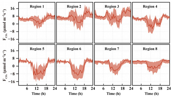
Figure 11.
Characterization of the annual average diurnal variation in for the eight regions of interest. The solid line is the average and the shading is the quartile.
3.6. Effect of Land Cover on CO2 Flux
Figure 12 analyzes the area ratio of the major carbon sink (vegetation = S1) and the major carbon source (the sum of the areas of buildings and main traffic roads = S2) on in each sector, and the results show that reached a maximum when S1/S2 reached a ratio of 1.8, and then decreased with the growth of the ratio after S1/S2 > 1.8 times. This shows that when the proportion of vegetation in the region was large enough, the carbon dioxide content in the atmosphere could be reduced.

Figure 12.
The impact of vegetation area/building and transportation trunk road area on ; ratio values are binned in 0.5 times increments.
4. Discussion
4.1. Factors Affecting Temporal Variation in CO2 Flux
variations at urban sites follow a seasonal cycle. Study sites in Portugal [39], Swindon [40] and Arnhem [1] found that was significantly higher in winter than in other seasons. In the present study site, the average value of was highest in winter and lowest in summer, which was regulated by plant photosynthesis [11,18,41]. The increase in PAR will promote the photosynthesis rate of plants [40]. Crawford et al. [42] found that when PAR reached a high value, tended to be stable. There was a significant correlation between PAR and at this site (p < 0.01), but the rate of response to PAR was different in different seasons. After PAR reached 1500, and 830 μmol·m−2·s−1 in summer and autumn, respectively, increased with the increase in PAR, indicating that excessive PAR would promote the recovery of . This may be because high PAR promotes the increase in VPD and causes the stomata of plant leaves to close, which inhibits CO2 uptake by plants; on the other hand, the soil temperature rises too rapidly during high PAR, which increases the heterotrophic respiration of the ecosystem and leads to the increase in [35].
VPD and Tair regulate the rate of response to PAR [43]. VPD affects the photosynthetic rate of vegetation by regulating the stomatal conductance of vegetation and the moisture conditions at the atmosphere–soil interface, which in turn affects the photosynthetic rate of vegetation [44]. Wang et al. [45] found that excessive VPD affects the rate of response to PAR by hindering photosynthesis in plants, and thus affects the rate of response to PAR. In this study, when PAR ≤ 1400 μmol·m−2·s−1, the rate of response to PAR decreased with increasing VPD, indicating that high VPD inhibited the rate of photosynthesis in plants. However, when PAR > 1400 μmol·m−2·s−1 and VPD ≤ 5 hpa, the rate of response of to PAR changes slowed down and leveled off. This may be because the plant photosynthesis has reached saturation and the photosynthetic rate of the plant no longer changes with the increase in PAR [37,40]. In addition, the response of to PAR changes was lowest when PAR ≤ 1300 μmol·m−2·s−1 and Tair > 16 °C, indicating that high temperatures inhibited the rate of response to PAR, which was consistent with the findings of Carrara et al. [46]. High temperatures were usually accompanied by higher VPD, resulting in a decrease in the carbon sequestration capacity of vegetation and reduced CO2 uptake [46].
The temporal variation characteristics of in cities are related to the intensity of human activities, and anthropogenic emissions are mainly through vehicle emissions and gas consumption [40,47]. Takano et al. [17] and Ueyama et al. [48] found that more frequent traffic flows during the daytime resulted in higher than at night during the diurnal variation in . During this study period, the average was higher at night than during the day and the difference between day and night ranged from 1.02 to 9.16 μmol·m−2·s−1. This phenomenon usually occurred in suburban or forested areas [49,50], which indicated the high vegetation cover (43.5%) at this study site. In addition, traffic flow affected the diurnal and cyclic characteristics of , with two peaks in the morning and evening diurnal variation, and lower on weekends than on weekdays [48]. Significant peaks were observed in the diurnal variation in in urban research sites in Mexico, Swindon, and Rhodes. The peak time of daytime during weekends / holidays lagged behind that of working days, and the diurnal average was smaller than that of working days [20,40,50]. The diurnal variation in at the present study site had peaks in the morning and evening, but the characteristics of the diurnal variation in between weekdays and weekends were similar and the differences in the average values were small, which may be due to the fact that the population of the study site consists of mainly students and residents, and most of the trips were on foot, which triggered fewer changes in the vehicular flow. This further indicates that flux changes in urban areas are jointly influenced by both anthropogenic and natural aspects. In particular, traffic flow is one of the main sources of anthropogenic emissions. Therefore, it is very important to reasonably regulate the development of urban transportation in the future to reduce carbon emissions [51,52].
4.2. Response of CO2 Flux to Spatial Variability
Due to the differences in anthropogenic activities and geography, CO2 emissions vary greatly even in different wind directions at the same site [17,37,53]. Velasco et al. [41] and Crawford et al. [42] found that the areas with frequent traffic flow and more exhaust emissions will lead to an increase in carbon dioxide content in the region. In regions of interest 1~3 where a main traffic artery road was present in this study, the level of annual average diurnal variation in was higher than the other regions of interest. This was consistent with the high level of in road areas found by Vesala et al. [18], which suggested that the main traffic artery road with high traffic volumes was the main cause of elevated in the regions of interest 1~3 of this study. As a major carbon sink area in the city, the vegetated subsurface absorbed atmospheric CO2 through plant photosynthesis, and thus absorbed atmospheric CO2 [45,54]. Liu et al. [55] found that the areas with a higher percentage of vegetation in the urban area of Beijing resulted in lower . Salgueiro et al. [39] in a study of coastal cities and suburbs in Portugal found that due to the influence of plant photosynthesis, a minimum was observed at midday and was much smaller in the suburbs than in the urban areas. In the present study, a decreasing trend in during midday hours was observed in all regions of interest during the annual average diurnal variation in , but the decrease in was greater in regions 4~6 (up to −9.4 μmol·m−2·s−1). This may be attributed to the high percentage of vegetation (48%~57%) in this region 4–6, which is well irrigated, resulting in a higher CO2 uptake capacity of the vegetation [56]. However, the decrease in during the midday hours was lower in region 4 than in regions 5~6, which may be due to the fact that region 4 was mainly residential, and the frequency of residential activities during the midday hours was higher. In addition, in this study, region 8 had the highest percentage of vegetation within the source area, but the carbon sink capacity of vegetation was much lower than that of regions 5~6 during the midday hours, which may be due to the fact that this area had a driveway facing the school gate (categorized as other impervious land), and the frequent traffic in and out of the school increased CO2 emissions from this area.
in urban areas is regulated by the size of buildings, roads, and vegetation, with increasing with the size of buildings and roads, and decreasing with the size of vegetation [43,57]. Therefore, understanding the ratio of carbon source areas to carbon sink areas in cities is useful in providing directions for the construction of sustainable urban development in the future. Crawford et al.’s [42] study in Baltimore found that higher was observed in the southwest direction with dense buildings and a high proportion of roads, while lower was observed in the northeast direction with more vegetation. This study further analyzed the effect of the area ratio between carbon sinks (plants) and carbon sources (buildings and roads) on , which showed a decreasing trend when the area ratio of the study site reached 1.8 times. It indicated that when the vegetation ratio at the study site was large enough, the atmospheric CO2 content would decrease. This may be because more CO2 in the atmosphere was absorbed as the photosynthetic capacity of plants increased with the increase in vegetation area [48]. Therefore, in future urban planning, the green area can be appropriately increased to mitigate atmospheric CO2. However, due to the spatial heterogeneity of the city, the results of our study at this site can only represent the state of similar urban functional units or ecosystems to a certain extent, but not the whole city. Therefore, it is necessary to set up multiple observation stations for different functional and ecosystem types in cities to improve the observation results to provide the most objective and extensive data support for accurate estimation of urban carbon emissions and identification of carbon sources and sinks.
The heterogeneity of the urban surface is extremely high, and there are great differences in anthropogenic activities and natural factors in different wind directions. The observed by the EC system depends on the wind direction, which may cause the observed ) to be high or low due to the influence of the wind direction frequency [48,55,58]. Pawlak et al. [50] found that the main wind direction was west and southwest in the study site in Łódź, Poland, but the observed in the east was nearly four times higher than that in the west. Kleingeld et al.’s [1] study in Arnhem found that the in the direction of busy traffic artery roads was higher. Therefore, these studies illustrated the potential for observed to be unrepresentative of the entire source area if the study area had a prevailing wind direction. In this study, 60% of the flux data came from the northwest. In order to verify whether the observations at the study site were representative of the source region, two approaches were used in this paper. One was based on the flux data every 30 min after the observation data had been processed, averaging the at each moment to obtain the annual average diurnal variation characteristics of within the source region. The other approach averaged the at each moment during the annual average diurnal variation in the eight regions of interest again, and thus obtained the annual average diurnal variation characteristics within the source region. Compared with the first approach, the second approach eliminated the effect of wind direction and better characterized the diurnal variation in within the source area. However, the comparison revealed that the annual average diurnal variation in obtained by the two approaches had the same trend (Figure 13) and the correlation was very high (R2 = 0.98, p < 0.01), which indicated that the observed at the present study site was not limited by the wind direction.

Figure 13.
Characterization of the annual average diurnal variation in . (a) Based on observed data; (b) based on eight regions of interest, with solid lines as averages and shaded quartiles.
5. Conclusions
This paper analyzed the variations of and its influencing factors based on the and meteorological data continuously monitored from January to December 2012 at the urban ecological station of the Central South University of Forestry Science and Technology in Changsha. The results showed that the source area was a net CO2 emission source all year round, and the flux footprint was mainly concentrated in the 500 m range, which was characterized by a typical urban subsurface. The diurnal variation characteristics of showed great differences in different time scales, but with a time-varying pattern, which was mainly because the photosynthesis capacity of plants was influenced by PAR and indirectly regulated by Tair and VPD, resulting in regular changes in the atmospheric CO2 content. In addition, in the changing pattern of in a day, it was obvious that it was also affected by the traffic flow with the phenomenon of morning and evening peaks. The land use of the surface is an important factor affecting the spatial variation in , and in this study area, the region 4~6 with higher vegetation occupation obviously had a larger diurnal variation in , with an obvious carbon sink process in the middle of the day, whereas the regions 1~3 with high traffic flow had a smaller variation in and were basically in the carbon source. It indicated that transportation was the main source of CO2 emission in the region, while vegetation can effectively mitigate the CO2 content in the region. By further discussing the impact of major carbon sources and sinks on the area, it was found that the CO2 content of the area would decrease after the area was covered by vegetation 1.8 times the sum of the areas of buildings and main traffic roads. This finding may provide a reference for the development of targeted carbon reduction strategies in the future.
Author Contributions
Z.D.: conceptualization, methodology, formal analysis, data curation, writing—original draft and writing—review and editing. X.L. (Xin Liu) and H.Z.: software and visualization. Y.C., J.L., M.Y. and X.W.: software. X.L. (Xiaocui Liang): writing—review and editing. X.Z. and W.Y.: methodology, resources, writing—review and editing, validation, supervision, and funding acquisition. All authors have read and agreed to the published version of the manuscript.
Funding
This research was funded by “Scientific Research Program of the Department of Education of Hunan Province, grant number 20B604”, “Joint Funds of the National Natural Science Foundation of China, grant number U21A20187”, “National Key R&D Program of China, grant number 2020YFA0608100”, “the Project for Central Financial Forestry Science and Technology Promotion Demonstration, grant number [2023]XT 08”, “Key Research and Development Program of Hunan Province, grant number 2023SK2055”, “Water Science and Technology Project of Hunan Province, grant number XSKJ2022068-35”, and “the Scientific Innovation Fund for Postgraduates of Central South University of Forestry and Technology, grant number 2023CX02059”.
Data Availability Statement
Data sharing is not applicable to this article.
Acknowledgments
We gratefully acknowledge the kind support of the National Engineering Laboratory for Applied Technology of Forestry and Ecology in South China and the Key Laboratory of Urban Forest Ecology of Hunan Province.
Conflicts of Interest
The authors declare no conflict of interest.
References
- Kleingeld, E.; van Hove, B.; Elbers, J.; Jacobs, C. Carbon dioxide fluxes in the city centre of Arnhem, A middle-sized Dutch city. Urban Clim. 2018, 24, 994–1010. [Google Scholar] [CrossRef]
- Kordowski, K.; Kuttler, W. Carbon dioxide fluxes over an urban park area. Atmos. Environ. 2010, 44, 2722–2730. [Google Scholar] [CrossRef]
- Song, J.Y.; Wang, Z.-H.; Wang, C.H. Biospheric and anthropogenic contributors to atmospheric CO2 variability in a residential neighborhood of Phoenix, Arizona. J. Geophys. Res. Atmos. 2017, 122, 3317–3329. [Google Scholar] [CrossRef]
- Tan, J.G.; Zheng, Y.F.; Tang, X.; Guo, C.Y.; Li, L.P.; Song, G.X.; Zhen, X.R.; Yuan, D.; Kalkstein, A.J.; Li, F.R.; et al. The urban heat island and its impact on heat waves and human health in Shanghai. Int. J. Biometeorol. 2010, 54, 75–84. [Google Scholar] [CrossRef] [PubMed]
- Li, D.; Bou-Zeid, E. Synergistic Interactions between Urban Heat Islands and Heat Waves: The Impact in Cities Is Larger than the Sum of Its Parts. J. Appl. Meteorol. Climatol. 2013, 52, 2051–2064. [Google Scholar] [CrossRef]
- Wu, K.; Yang, X.Q. Urbanization and heterogeneous surface warming in eastern China. Chin. Sci. Bull. 2013, 58, 1363–1373. [Google Scholar] [CrossRef]
- Helfter, C.; Famulari, D.; Phillips, G.; Barlow, J.; Wood, C.; Grimmond, S.; Nemitz, E. Controls of carbon dioxide concentrations and fluxes above central London. Atmos. Chem. Phys. Discuss. 2010, 11, 1913–1928. [Google Scholar] [CrossRef]
- Kotthaus, S.; Grimmond, C.S.B. Energy exchange in a dense urban environment—Part I: Temporal variability of long-term observations in central London. Urban Clim. 2014, 10, 261–280. [Google Scholar] [CrossRef]
- Velasco, E.; Perrusquia, R.; Jiménez, E.; Hernández, F.; Camacho, P.; Rodríguez, S.; Retama, A.; Molina, L.T. Sources and sinks of carbon dioxide in a neighborhood of Mexico City. Atmos. Environ. 2014, 97, 226–238. [Google Scholar] [CrossRef]
- Baldocchi, D.D. ‘Breathing’ of the terrestrial biosphere: Lessons learned from a global network of carbon dioxide flux measurement systems. Aust. J. Bot. 2008, 56, 1–26. [Google Scholar] [CrossRef]
- Bergeron, O.; Strachan, I.B. CO2 sources and sinks in urban and suburban areas of a northern mid-latitude city. Atmos. Environ. 2011, 45, 1564–1573. [Google Scholar] [CrossRef]
- Christen, A.; Coops, N.C.; Crawford, B.R.; Kellett, R.; Liss, K.N.; Olchovski, I.; Tooke, T.R.; van der Laan, M.; Voogt, J.A. Validation of modeled carbon-dioxide emissions from an urban neighborhood with direct eddy-covariance measurements. Atmos. Environ. 2011, 45, 6057–6069. [Google Scholar] [CrossRef]
- Soegaard, H.; Møller-Jensen, L. Towards a spatial CO2 budget of a metropolitan region based on textural image classification and flux measurements. Remote Sens. Environ. 2003, 87, 283–294. [Google Scholar] [CrossRef]
- Crawford, B.; Christen, A. Spatial source attribution of measured urban eddy covariance CO2 fluxes. Theor. Appl. Climatol. 2015, 119, 733–755. [Google Scholar] [CrossRef]
- Feigenwinter, C.; Vogt, R.; Christen, A. Eddy Covariance Measurements Over Urban Areas. In Eddy Covariance: A Practical Guide to Measurement and Data Analysis; Aubinet, M., Vesala, T., Papale, D., Eds.; Springer: Dordrecht, The Netherlands, 2012; pp. 377–397. [Google Scholar] [CrossRef]
- Vogt, R.; Christen, A.; Rotach, M.W.; Roth, M.; Satyanarayana, A.N.V. Temporal dynamics of CO2 fluxes and profiles over a Central European city. Theor. Appl. Climatol. 2006, 84, 117–126. [Google Scholar] [CrossRef]
- Takano, T.; Ueyama, M. Spatial variations in daytime methane and carbon dioxide emissions in two urban landscapes, Sakai, Japan. Urban Clim. 2021, 36, 100798. [Google Scholar] [CrossRef]
- Vesala, T.; Kljun, N.; Rannik, Ü.; Rinne, J.; Sogachev, A.; Markkanen, T.; Sabelfeld, K.; Foken, T.; Leclerc, M.Y. Flux and concentration footprint modelling: State of the art. Environ. Pollut. 2008, 152, 653–666. [Google Scholar] [CrossRef]
- Kurppa, M.; Nordbo, A.; Haapanala, S.; Järvi, L. Effect of seasonal variability and land use on particle number and CO2 exchange in Helsinki, Finland. Urban Clim. 2015, 13, 94–109. [Google Scholar] [CrossRef]
- Velasco, E.; Pressley, S.; Grivicke, R.; Allwine, E.; Coons, T.; Foster, W.; Jobson, B.T.; Westberg, H.; Ramos, R.; Hernández, F.; et al. Eddy covariance flux measurements of pollutant gases in urban Mexico City. Atmos. Chem. Phys. 2009, 9, 7325–7342. [Google Scholar] [CrossRef]
- Chrysoulakis, N.; Grimmond, S.; Feigenwinter, C.; Lindberg, F.; Gastellu-Etchegorry, J.-P.; Marconcini, M.; Mitraka, Z.; Stagakis, S.; Crawford, B.; Olofson, F.; et al. Urban energy exchanges monitoring from space. Sci. Rep. 2018, 8, 11498. [Google Scholar] [CrossRef]
- Chrysoulakis, N.; Lopes, M.; San José, R.; Grimmond, C.S.B.; Jones, M.B.; Magliulo, V.; Klostermann, J.E.M.; Synnefa, A.; Mitraka, Z.; Castro, E.A.; et al. Sustainable urban metabolism as a link between bio-physical sciences and urban planning: The BRIDGE project. Landsc. Urban Plan. 2013, 112, 100–117. [Google Scholar] [CrossRef]
- Christen, A.; Coops, N.; Canada Research Chairs, O.O.N.; Kellet, R. LIDAR-Based Urban Metabolism Approach to Neighbourhood Scale Energy and Carbon Emissions Modelling; Western Ontario Univ.: London, ON, Canada, 2010. [Google Scholar]
- Grimmond, C.S.B.; King, T.S.; Cropley, F.D.; Nowak, D.J.; Souch, C. Local-scale fluxes of carbon dioxide in urban environments: Methodological challenges and results from Chicago. Environ. Pollut. 2002, 116, S243–S254. [Google Scholar] [CrossRef] [PubMed]
- Grimm, N.B.; Faeth, S.H.; Golubiewski, N.E.; Redman, C.L.; Wu, J.; Bai, X.; Briggs, J.M. Global change and the ecology of cities. Science 2008, 319, 756–760. [Google Scholar] [CrossRef] [PubMed]
- Ao, X.Y.; Grimmond, C.S.B.; Chang, Y.Y.; Liu, D.W.; Tang, Y.Q.; Hu, P.; Wang, Y.D.; Zou, J.; Tan, J.G. Heat, water and carbon exchanges in the tall megacity of Shanghai: Challenges and results. Int. J. Climatol. 2016, 36, 4608–4624. [Google Scholar] [CrossRef]
- Dijk, A.; Moene, A.F.; de Bruin, H. The Principles of Surface Flux Physics: Theory, Practice and Description of the ECPACK Library; Internal Report 2004/1; Meteorology and Air Quality Group, Wageningen University: Wageningen, The Netherlands, 2004; pp. 30–54. Available online: http://www.met.wau.nl/projects/jep (accessed on 27 September 2023).
- Moncrieff, J.B.; Massheder, J.M.; de Bruin, H.; Elbers, J.; Friborg, T.; Heusinkveld, B.; Kabat, P.; Scott, S.; Soegaard, H.; Verhoef, A. A system to measure surface fluxes of momentum, sensible heat, water vapour and carbon dioxide. J. Hydrol. 1997, 188–189, 589–611. [Google Scholar] [CrossRef]
- Moncrieff, J.; Clement, R.; Finnigan, J.; Meyers, T. Averaging, Detrending, and Filtering of Eddy Covariance Time Series. In Handbook of Micrometeorology: A Guide for Surface Flux Measurement and Analysis; Lee, X., Massman, W., Law, B., Eds.; Springer: Dordrecht, The Netherlands, 2005; pp. 7–31. [Google Scholar]
- Webb, E.K.; Pearman, G.I.; Leuning, R. Correction of flux measurements for density effects due to heat and water vapour transfer. Q. J. R. Meteorol. Soc. 1980, 106, 85–100. [Google Scholar] [CrossRef]
- Mauder, M.; Foken, T. Impact of post-field data processing on eddy covariance flux estimates and energy balance closure. Meteorol. Z. 2006, 15, 597–609. [Google Scholar] [CrossRef]
- Grimmond, C.S.B.; Salmond, J.A.; Oke, T.R.; Offerle, B.; Lemonsu, A. Flux and turbulence measurements at a densely built-up site in Marseille: Heat, mass (water and carbon dioxide), and momentum. J. Geophys. Res. Atmos. 2004, 109. [Google Scholar] [CrossRef]
- Papale, D.; Reichstein, M.; Aubinet, M.; Canfora, E.; Bernhofer, C.; Kutsch, W.; Longdoz, B.; Rambal, S.; Valentini, R.; Vesala, T.; et al. Towards a standardized processing of Net Ecosystem Exchange measured with eddy covariance technique: Algorithms and uncertainty estimation. Biogeosciences 2006, 3, 571–583. [Google Scholar] [CrossRef]
- Isaac, P.; Cleverly, J.; McHugh, I.; van Gorsel, E.; Ewenz, C.; Beringer, J. OzFlux data: Network integration from collection to curation. Biogeosciences 2017, 14, 2903–2928. [Google Scholar] [CrossRef]
- Reichstein, M.; Falge, E.; Baldocchi, D.; Papale, D.; Aubinet, M.; Berbigier, P.; Bernhofer, C.; Buchmann, N.; Gilmanov, T.; Granier, A.; et al. On the separation of net ecosystem exchange into assimilation and ecosystem respiration: Review and improved algorithm. Glob. Chang. Biol. 2005, 11, 1424–1439. [Google Scholar] [CrossRef]
- Kljun, N.; Calanca, P.; Rotach, M.W.; Schmid, H.P. A Simple Parameterisation for Flux Footprint Predictions. Bound.-Layer Meteorol. 2004, 112, 503–523. [Google Scholar] [CrossRef]
- Ward, H.C.; Kotthaus, S.; Grimmond, C.S.B.; Bjorkegren, A.; Wilkinson, M.; Morrison, W.T.J.; Evans, J.G.; Morison, J.I.L.; Iamarino, M. Effects of urban density on carbon dioxide exchanges: Observations of dense urban, suburban and woodland areas of southern England. Environ. Pollut. 2015, 198, 186–200. [Google Scholar] [CrossRef]
- Mobbs, S.D. Introduction to Micrometeorology, S.P.; Arya, Academic Press (San Diego), 1988. No. of Pages: 307. Price US $39.95. Int. J. Climatol. 1991, 11, 223–224. [Google Scholar] [CrossRef]
- Salgueiro, V.; Cerqueira, M.; Monteiro, A.; Alves, C.; Rafael, S.; Borrego, C.; Pio, C. Annual and seasonal variability of greenhouse gases fluxes over coastal urban and suburban areas in Portugal: Measurements and source partitioning. Atmos. Environ. 2020, 223, 117204. [Google Scholar] [CrossRef]
- Ward, H.C.; Evans, J.G.; Grimmond, C.S.B. Multi-season eddy covariance observations of energy, water and carbon fluxes over a suburban area in Swindon, UK. Atmos. Chem. Phys. 2013, 13, 4645–4666. [Google Scholar] [CrossRef]
- Velasco, E.; Roth, M. Cities as Net Sources of CO2: Review of Atmospheric CO2 Exchange in Urban Environments Measured by Eddy Covariance Technique. Geogr. Compass 2010, 4, 1238–1259. [Google Scholar] [CrossRef]
- Crawford, B.; Grimmond, C.S.B.; Christen, A. Five years of carbon dioxide fluxes measurements in a highly vegetated suburban area. Atmos. Environ. 2011, 45, 896–905. [Google Scholar] [CrossRef]
- Järvi, L.; Nordbo, A.; Junninen, H.; Riikonen, A.; Moilanen, J.; Nikinmaa, E.; Vesala, T. Seasonal and annual variation of carbon dioxide surface fluxes in Helsinki, Finland, in 2006–2010. Atmos. Chem. Phys. 2012, 12, 8475–8489. [Google Scholar] [CrossRef]
- Cao, S.K.; Cao, G.C.; Feng, Q.; Han, G.Z.; Lin, Y.Y.; Yuan, J.; Wu, F.T.; Cheng, S.Y. Alpine wetland ecosystem carbon sink and its controls at the Qinghai Lake. Environ. Earth Sci. 2017, 76, 210. [Google Scholar] [CrossRef]
- Wang, Y.Y.; Ma, Y.M.; Li, H.X.; Yuan, L. Carbon and water fluxes and their coupling in an alpine meadow ecosystem on the northeastern Tibetan Plateau. Theor. Appl. Climatol. 2020, 142, 1–18. [Google Scholar] [CrossRef]
- Carrara, A.; Janssens, I.A.; Curiel Yuste, J.; Ceulemans, R. Seasonal changes in photosynthesis, respiration and NEE of a mixed temperate forest. Agric. For. Meteorol. 2004, 126, 15–31. [Google Scholar] [CrossRef]
- Gioli, B.; Toscano, P.; Lugato, E.; Matese, A.; Miglietta, F.; Zaldei, A.; Vaccari, F.P. Methane and carbon dioxide fluxes and source partitioning in urban areas: The case study of Florence, Italy. Environ. Pollut. 2012, 164, 125–131. [Google Scholar] [CrossRef] [PubMed]
- Ueyama, M.; Ando, T. Diurnal, weekly, seasonal, and spatial variabilities in carbon dioxide flux in different urban landscapes in Sakai, Japan. Atmos. Chem. Phys. 2016, 16, 14727–14740. [Google Scholar] [CrossRef]
- Thomas, M.V.; Malhi, Y.; Fenn, K.M.; Fisher, J.B.; Morecroft, M.D.; Lloyd, C.R.; Taylor, M.E.; McNeil, D.D. Carbon dioxide fluxes over an ancient broadleaved deciduous woodland in southern England. Biogeosciences 2011, 8, 1595–1613. [Google Scholar] [CrossRef]
- Pawlak, W.; Fortuniak, K.; Siedlecki, M. Carbon dioxide flux in the centre of Łódź, Poland—Analysis of a 2-year eddy covariance measurement data set. Int. J. Climatol. 2011, 31, 232–243. [Google Scholar] [CrossRef]
- Sharifi, A. Co-benefits and synergies between urban climate change mitigation and adaptation measures: A literature review. Sci. Total Environ. 2021, 750, 141642. [Google Scholar] [CrossRef]
- Sun, C.; Zhang, Y.; Ma, W.; Wu, R.; Wang, S. The Impacts of Urban Form on Carbon Emissions: A Comprehensive Review. Land 2022, 11, 1430. [Google Scholar] [CrossRef]
- Min, K.E.; Mun, J.; Perdigones, B.; Lee, S.; Kwak, K.H. Insights on estimating urban CO2 emissions using eddy-covariance flux measurements. Atmos. Chem. Phys. Discuss. 2022, 2022, 1–24. [Google Scholar] [CrossRef]
- Nordbo, A.; Järvi, L.; Haapanala, S.; Moilanen, J.; Vesala, T. Intra-City Variation in Urban Morphology and Turbulence Structure in Helsinki, Finland. Bound.-Layer Meteorol. 2013, 146, 469–496. [Google Scholar] [CrossRef]
- Liu, H.Z.; Feng, J.W.; Jrvi, L.; Vesala, T. Four-year (2006–2009) eddy covariance measurements of CO2 flux over an urban area in Beijing. Atmos. Chem. Phys. 2012, 12, 7881–7892. [Google Scholar] [CrossRef]
- Pérez-Ruiz, E.R.; Vivoni, E.R.; Templeton, N.P. Urban land cover type determines the sensitivity of carbon dioxide fluxes to precipitation in Phoenix, Arizona. PLoS ONE. 2020, 15, e0228537. [Google Scholar] [CrossRef] [PubMed]
- Coutts, A.M.; Beringer, J.; Tapper, N.J. Characteristics influencing the variability of urban CO2 fluxes in Melbourne, Australia. Atmos. Environ. 2007, 41, 51–62. [Google Scholar] [CrossRef]
- Kotthaus, S.; Grimmond, C.S.B. Identification of Micro-scale Anthropogenic CO2, heat and moisture sources–Processing eddy covariance fluxes for a dense urban environment. Atmos. Environ. 2012, 57, 301–316. [Google Scholar] [CrossRef]
Disclaimer/Publisher’s Note: The statements, opinions and data contained in all publications are solely those of the individual author(s) and contributor(s) and not of MDPI and/or the editor(s). MDPI and/or the editor(s) disclaim responsibility for any injury to people or property resulting from any ideas, methods, instructions or products referred to in the content. |
© 2023 by the authors. Licensee MDPI, Basel, Switzerland. This article is an open access article distributed under the terms and conditions of the Creative Commons Attribution (CC BY) license (https://creativecommons.org/licenses/by/4.0/).