An SSD-MobileNet Acceleration Strategy for FPGAs Based on Network Compression and Subgraph Fusion

Abstract

Over the last decade, various deep neural network models have achieved great success in image recognition and classification tasks. The vast majority of high-performing deep neural network models have a huge number of parameters and often require sacrificing performance and accuracy when they are deployed on mobile devices with limited area and power consumption. To address this problem, we present an SSD-MobileNet-v1 acceleration method based on network compression and subgraph fusion for Field-Programmable Gate Arrays (FPGAs). Firstly, a regularized pruning algorithm based on sensitivity analysis and Filter Pruning via Geometric Median (FPGM) was proposed. Secondly, the Quantize Aware Training (QAT)-based network full quantization algorithm was designed. Finally, a strategy for computing subgraph fusion is proposed for FPGAs to achieve continuous scheduling of Programmable Logic (PL) operators. The experimental results show that using the proposed acceleration strategy can reduce the number of model parameters by a factor of 11 and increase the inference speed on the FPGA platform by a factor of 9–10. The acceleration algorithm is applicable to various mobile edge devices and can be applied to the real-time monitoring of forest fires to improve the intelligence of forest fire detection.

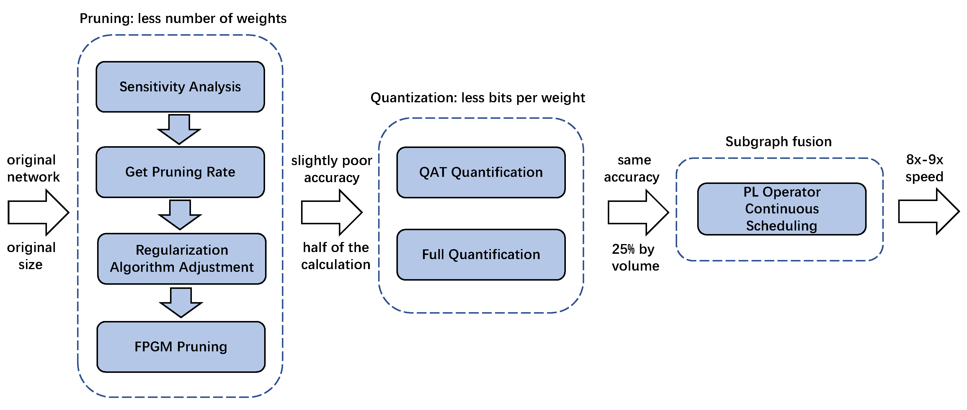
1. Introduction

Forest fires have the characteristics of being widespread, sudden, and challenging to extinguish. It is of great significance to find the fire point in time and extinguish it as soon as possible to avoid a major forest disaster. At present, most monitoring systems use sensors such as temperature-sensitive, smoke-sensitive, light-sensitive, and composite sensors. These sensors have good results in specific scenarios but they also have several shortcomings, for example, they have long response times, are prone to being misreported, and have a limited scope of application. Infrared and ultraviolet cameras used to detect forest fires have the characteristics of fast response times and high sensitivity, but they are easily obstructed by radiation sources in other complex environments and have high costs. Therefore, it is still a challenge to carry out efficient, accurate, and real-time detection in large forested areas [1].

With the development of deep learning technology [2,3,4,5], people have gradually applied various deep learning algorithms to forest fire detection. Taking convolutional neural networks (CNN) for image and video detection as an example, they have the characteristics of high recognition rates and wide recognition ranges, but at the same time, the trouble is that they involve huge computational costs [6]. Particularly in recent years, in order to improve the performance of convolutional neural networks, researchers have been trying to increase the depth and width of convolutional neural networks. For example, as shown in

Table 1. Comparison of classical CNN models on ImageNet.

Model	Layer Number	Size/MB	Flops	Parameters/M	ImageNet Top 5 Error Rates/%
AlexNet	8	>200	1.5	60	16.4
VGG	19	>500	19.6	138	7.32
GoogleNet	22	50	1.556	6.8	6.67
ResNet	152	230	11.3	19.4	3.57

, VGG [7] deepens the network structure based on AlexNet [8], increasing the number of network layers from 8 to 19; GoogLeNet [9] proposes an inception module to broaden the network model; and ResNet [10] increases the network to 152 layers and proposes a residual module. Although these networks have improved performance, they also increase the number of parameters. If all the image data are transmitted to the server for computing, it is a challenge due not only to the required network transmission and cloud computing but also the real-time accuracy and reliability of recognition. Edge computing services can run directly on a terminal device, which solves the problems of the high latency, network instability, and low bandwidth of the traditional cloud-computing mode. They are especially suitable for business applications that are sensitive to high computation loads, delays, and data security concerns. An FPGA is one of the mainstream chips that can support edge computing services [11]. FPGAs have the natural advantages of low latency and stability, and the hardware costs are not high. They are more suitable for edge computing scenarios for forest fire detection than other heterogeneous processors. However, when using neural networks in forest fire detection, we should consider not only the accuracy of the network for forest fire identification but also the need to balance the contradiction between the huge number of calculations brought about by the good performance of the network and the limited computing power of the FPGA platform, which also increases the difficulty of deploying convolutional neural networks on FPGA mobile platforms [12].

Therefore, ways of reducing the storage space of network models and improving the speed of network reasoning under the condition of ensuring or reducing the performance of neural networks have become urgent problems that need to be solved. Therefore, neural network compression technology [13] came into being. At present, network compression methods are mainly divided into network pruning [14,15], network parameter quantization and decomposition [16,17], the lightweight design of the network structure [18,19,20], and knowledge distillation [21]. Pruning is one of the mainstream methods for neural network compression, mainly for the neural network structure itself, which can adjust and trim, remove unimportant parameters, and effectively reduce the number of parameters and calculations. Quantization uses fixed-point (8-bit) reasoning to quantify the floating-point (float32) model in the model reasoning process, which can reduce the file size, memory occupied by the model’s files by 75%, and computing resources and power consumption required for reasoning calculations. Of course, both methods can cause a loss of precision.

In view of the above problems, the purposes of this paper are to use the neural network compression technology methods of pruning and quantification on the SSD-MobileNet-v1 network model while ensuring the accuracy of the model, as well as reduce the number of parameters and calculations and compress the volume of the model. The size, along with the subgraph fusion strategy, improves the reasoning speed of the network model on the FPGA platform, thereby reducing the difficulty of deployment, improving the practicability of the FPGA platform for forest fire detection, and improving the real-time accuracy and intelligence of forest fire detection. Firstly, the lightweight network MobileNet [19] is used to replace the Visual Geometry Group (VGG) [7] as the basic network for extracting network features in the Single Shot MultiBox Detector (SSD) [22] algorithm to form a new SSD-MobileNet-v1 network structure. The main idea of MobileNet [23] is to use deep separable convolution instead of standard convolution, which decomposes standard convolution into deep convolution and point convolution. The deep convolution filter performs a single convolution on each input channel, and the point convolution filter linearly combines the output of the deep convolution with the 1 × 1 convolution. Suppose the size of the standard convolution kernel is $D_K$; when the number of convolution kernels is N , the ratio W of the computational complexity of depthwise separable convolution and standard convolution is $\frac{1}{N}+\frac{1}{K^2}$ [23]. The $D_K$ of different convolutional layer filters in the MobileNet network is 3 × 3, and the number of convolution kernels N is much larger than $D_K$. Therefore, compared to standard convolution, the computational complexity of depth-level separable convolution is reduced 8–9-fold. The follow-up work is shown in Figure 1. Compared to weight pruning, channel pruning can obtain a regular model and the parameters are easy to control. Therefore, this paper uses the input–output relationship of the network to obtain statistical information. After the sensitivity analysis of the network, the regular pruning method based on FPGM is used to prune the neural network at the filter level, reducing the number of calculations by half. The pruned model is then fully compressed based on QAT to about one-tenth the size of the original SSD-MobileNet-v1 model. Finally, subgraph fusion is carried out on the model to be deployed and the strategy of the continuous scheduling of the PL operator is realized through subgraph fusion, significantly increasing the inference speed of the network deployment on the hardware platform.

2. Related Works

In large-scale network models, there is always a lot of weight redundancy, which greatly affects the computational efficiency, wastes computational resources, and even reduces the accuracy of the model. Therefore, we need to use a pruning method to compress the model. Under the condition of an appropriate compression rate, we can simultaneously improve the accuracy of the model and reduce its size. At the same time, when deploying the model on the mobile terminal, we also consider sacrificing some accuracy in exchange for time and space savings. Nowadays, there are many studies on neural network pruning and many network pruning methods have been proposed. Li et al. [24] proposed a method of L1 norm channel pruning, which uses an L1 norm evaluation to prune the convolution kernel, which does not cause sparse connections but is limited by the norm rules and some special weights are not applicable. Luo et al. [25] designed the ThiNet pruning method using a greedy strategy combined with a minimizing reconstruction error, which had a good pruning effect on ResNet50 and VGG16. He et al. [26] reduced the channel information in the input convolution map and used the lasso regression channel selection method and least squares reconstruction for effective network pruning. Liu et al. [27] proposed a pruning method for evaluating the importance of convolution for the $\gamma$ parameter of the batch normalization (BN) layer, which can only be pruned for networks with BN layers. Considering the limitations of the evaluation criteria of constant canonical numbers, He et al. [28] proposed a new FPGM pruning algorithm. This algorithm is only an evaluation criterion for the importance of the convolution kernel in the convolution layer and needs to be combined with other algorithms.

Another neural network model compression acceleration method is to compress the parameters by quantifying them to accelerate the neural network and reduce the computational costs [24]. In the literature [16], a complete description of the quantization process was proposed, which replaces the floating-point weight in the neural network with a 1-bit binary weight (−1, 1), which can simplify the multiplication operation into a simple accumulation operation through hardware calculation. However, the algorithm only achieves an accuracy loss on small datasets such as MNIST, CIFA-10, and SVHN. In [29], Binary Weight Networks (BWN) quantified the network weights to 1 bit but also multiplied the scale factor when the weights were quantified, thereby transforming the quantization problem into an optimization problem. In [30], TWNs quantified the weight parameters of the network model to 2 bits and the quantization value range was (1, 0, $-1$). Although this method could greatly compress the network model, the network detection accuracy was seriously reduced. Aiming at the problems of insufficient capacity and serious loss of model accuracy in the binary quantization algorithm proposed by the former, in [31], INQ was proposed as a three-step quantization algorithm of network weights by grouping parameters, quantizing by group, and retraining. In [32], BNNs further quantified the activation value into 1 bit based on BinaryConnect [29], which not only reduced the memory consumption but also simplified many multiplication and addition operations into bit operations. Although this method reduced the time complexity, the binarization quantization lost some important information, resulting in a significant decrease in accuracy. The TSQ proposed in [33] was a two-step quantization algorithm. In the first step, the weight maintained the floating-point type and the activation value was quantified by the sparse quantization method. The second step regarded the weight quantization as a nonlinear least square problem and solved the weight quantization value iteratively. Vanhoucke et al. [34] proposed an 8-bit parameter quantization method, which could achieve a significant acceleration while achieving a minimal loss of accuracy. However, the compression effect of this method on the network model was not obvious enough. In order to reduce the accuracy loss caused by parameter quantization, Han et al. [14] proposed a method of sharing weights and index coding through weights to reduce the number of weights and storage space. In addition, the work in [35] is the official white paper on neural network quantization published by Google. In this paper, three quantization schemes, uniform quantizer, uniform symmetric quantizer, and stochastic quantizer, and two network quantization algorithms, post-training quantization and quantization perception, were proposed.

The above studies focus on pruning and quantifying the neural network model, respectively, but after pruning the neural network to obtain a network model with a sparse structure, the model parameters can be optimized again and the floating-point parameters can be quantified into fixed-point data to obtain further compression of the network model. Therefore, this paper reduces the volume of the network model more than 10-fold using the regular pruning strategy based on sensitivity analysis and FPGM and the model full quantization strategy based on QAT. In addition, the continuous scheduling strategy of the PL operator is realized using subgraph fusion and finally, the inference speed of the network deployment on the hardware platform is increased 8–9-fold.

3. FPGM and Regular Pruning Strategy Based on Sensitivity Analysis

In this paper, sensitivity analysis is used to analyze the pruning ratio of each layer network, and the importance of the single convolution layer convolution kernel is analyzed using the geometric median after the adjustment of the regular pruning algorithm.

3.1. Sensitivity Analysis

In deep learning, the sensitivity analysis strategy can be used to study the sensitivity of the state or output changes of a network model to the changes in the system parameters or surrounding conditions. Using the sensitivity obtained by this strategy to analyze the influence of the pruning proportion of the single-layer convolution kernel on the accuracy loss can not only effectively analyze the optimal pruning rate of each layer but also effectively suppress the shortcomings caused by equal proportion pruning.

As shown in Figure 2, if there are m convolution layers, the number of filters in each layer is different, assuming we perform a statistical analysis of the sensitivity of the first convolution layer. First, before disconnecting the filter for sensitivity analysis, the original accuracy of the complete model should be measured and recorded as As. Then, we randomly disconnect 10% (0.1) of the filter for conv 1 with the other conv unchanged, calculate the accuracy of the model at this time as An, and record the difference between the original accuracy and the changed accuracy as (As−An). Then, we restore the model to its original state and perform the same operation on the models with 20%, 30%, 40%, 50%, 60%, 70%, 80%, and 90% filters disconnected in turn. Finally, we do the same for the remaining convs successively.

Figure 3 shows the network pruning process based on sensitivity analysis. The program starts to give the experimental data, pre-training model, pruning rate, and sensitivity information and sets the initial boundary of the loss value as [0, 1]. Then, it ensures that the accuracy loss value of all pruning layers is consistent and uses the dichotomy to approximate and calculate the appropriate loss value. Then, we perform the following steps: enter the circulation body, take the set mean value of the upper and lower boundaries of the loss value, retrieve a group of pruning ratios from the sensitivity according to the loss value, take the values from 0.9 to 0.1, obtain the pruning rate of the intersection of the loss value of each layer and the sensitivity curve, calculate the flops value and the overall pruning rate of the model in this group of pruning rates, and restore the model to its original state. Finally, we judge the relationship between the pruning rate and the set pruning rate under this loss value. If they are not equal, we reset the upper and lower boundaries and enter the circulation body. If they are equal, we find the required pruning proportion, obtain the appropriate loss value, and prune the model according to the obtained pruning rate.

3.2. FPGM Pruning Strategy

In the n-dimensional space, there is a point a* that minimizes the sum of the Euclidean distances from the m points $a_1$, $a_2$, $a_3$, …, $a_m$, …, $a_i$ in the space, and then point a* is the geometric midpoint of these m points. The Euclidean distance of the x and y points in the n-dimensional space is described as

$${\left||x-y|\right|}_2=\sqrt{\sum _{i=1}^n{(x_i-y_i)}^2}$$

(1)

Then, the geometric median of these m points is expressed as

$$f\left(a^{*}\right)=\underset{x\in n}{min}f\left(x\right)=\underset{x\in n}{min}\sum _{i\in [1,n]}{\left||x-a_i|\right|}_2$$

(2)

For neural networks, it is assumed that the k-th network layer has N filters, as shown in Figure 4, for 3 × 3, where the Euclidean distance ${\left||F_1-F_2|\right|}_2$ of filter1 and filter2 is

$${\left||F_1-F_2|\right|}_2=\sqrt{\sum _{i,j=1}^3{[A_1(i,j)-A_2(i,j)]}^2}$$

(3)

The parameters (i, j) in the formula are the parameter coordinates in the filter.

The FPGM strategy understands each layer of the network as a multidimensional space and each filter as a point. There are K convolution layers in the network and the neural network of layer j has N convolution kernels $F_1$, $F_2$, …, $F_N$. Then, its geometric median $F_l$ can be expressed as

$$F_l(i,j)\in \underset{j\in [1,K]}{argmin}\sum _{i\in [1,N]}{\left||F_x-F_i|\right|}_2$$

(4)

where $F_x$ is the undetermined geometric median; i is the filter serial number; and j is the corresponding value of the conv convolution.

The geometric median of the neural network filter is calculated in this layer as the parameter index of the filter group to evaluate the importance of a single filter. The closer the geometric median, the easier it is to be replaced by other filters.

3.3. Regularize Pruning Strategy

The pruning method based on sensitivity analysis in this paper is the compression of the convolution layer. The parameters of the different convolution layers of the neural network vary greatly so the importance degrees and their influence on the accuracy are also different. Therefore, the sensitivity analysis method is used to distinguish the importance degree of each convolution layer and its influence on the accuracy. Through sensitivity analysis and the set accuracy loss, the corresponding pruning rate is obtained. Then, the geometric median is used to evaluate the importance of the single-layer convolution kernel, and the pruning rate of each layer calculated by the sensitivity is used to prune each layer of convolution.

In this paper, when the network model is deployed on the FPGA end, the input channel port is 16. Therefore, regular pruning means that the number of channels in the network layer is still a preset multiple of 16 after pruning, which is conducive to improving the reasoning speed of the model and reducing the memory occupation. Thus, after obtaining the corresponding pruning rate through sensitivity analysis, we need to use the regular pruning algorithm to fine tune the pruning rate to obtain a new pruning rate.

Figure 5 shows the overall process of the pruning method in this paper, and the specific steps are as follows. First, read the data and network and train the original model or read the pre-training model. Then, carry out sensitivity analysis on the network model. If there is saved sensitivity information, read the sensitivity information of the network. Otherwise, carry out sensitivity analysis and save it as a file. The pruning rate of each convolution layer is obtained based on the sensitivity, and the pruning rate of each layer is fine tuned using the regular pruning algorithm. According to the pruning rate, the convolution kernel of the corresponding proportion close to the geometric center of each convolution layer is removed. Finally, the pruned network is trained twice to restore the accuracy lost by pruning as much as possible.

Figure 6 shows the process of adjusting the pruning rate using the regular pruning algorithm. First, input the name of each convolution layer of the original network and the corresponding number of channels, and then read the name of each convolution layer to be pruned and the corresponding pruning rate. The pruning rate is multiplied by the original number of channels to obtain the number of pruning channels. The number of pruning channels is subtracted from the original number of channels to obtain the number of remaining channels. Then, the number of remaining channels is rounded to the nearest multiple of 16 to obtain the adjusted number of channels. Finally, the new pruning rate can be obtained by dividing the adjusted number of channels by the original number of channels.

However, through research and experiments, we found that in SSD-MobileNet-v1 networks, when adjusting the pruning rate, most network layers reduce the pruning rate to ensure that the remaining network layers are a multiple of 16. Therefore, in order to ensure the pruning rate on the basis of the sensitivity, we set a new coefficient O, which is defined as the number of remaining channels in each network layer divided by 16. When O is greater than 5, 16 is subtracted from the number of channels in this layer to ensure the overall pruning rate. Finally, we compare the total number of channels subtracted from the original network and the total number of channels subtracted from the current network and find that the number is equivalent, and the overall pruning rate of the network has no significant increase or decrease compared to the original.

4. Quantization and Computation Subgraph Fusion

4.1. Network Full Quantization Based on QAT Quantitative Training

The QAT model is quantized during the training process but requires a large amount of labeled sample data and a long time to train the model. In the model output stage, the quantization training method uses the idea of simulation quantization and the weight is updated in the process of model training to achieve the purpose of fitting and reducing the quantization error. In the model deployment stage, the quantization training method is consistent with the static offline quantization method, and the same prediction and reasoning method is used to achieve the same benefits in terms of storage space, reasoning speed, and computing memory. More importantly, the quantized training method has only a minimal impact on model accuracy. The quantization training process is carried out on the trained model, that is to say, after adding the quantization inverse quantization op to the trained model, the parameters are fine tuned with a small learning rate. In this section, we describe how to model quantized pruned networks during training and how this can be easily done using the automatic quantization tools in Paddle.

Simulated quantization is modeled in the backward pass. For quantization-aware training, we model the effect of quantization using simulated quantization operations, which consist of a quantizer followed by a de-quantizer, i.e.,

$$x_{out}=SimQuant\left(x\right)$$

(5)

$$=\Delta clamp(0,\left(N_{levels}\right)-1,round\left({\displaystyle \frac{x}{\Delta }}\right)-z)$$

(6)

Since the derivative of a simulated uniform quantizer function is zero almost everywhere, approximations are required to model a quantizer in the backward pass. An approximation that has worked well in practice is to model the quantizer as specified in the equation below for the purposes of defining its derivative (See Figure 7).

$$x_{out}=clamp(x_{min},x_{max},x)$$

(7)

The backward pass is modeled as a “straight through estimator”. Specifically,

$${\delta }_{out}={\delta }_{in}{I}_{x\in S}S:x:x_{mix}\le x\le x_{max}$$

(8)

where ${\delta }_{in}=\frac{\delta L}{{\delta }_{w_{out}}}$ is the backpropagation error of the loss with respect to the simulated quantizer output.

We model the effect of quantization using simulated quantization operations on both the weights and activations. For the backward pass, we use the straight-through estimator to model quantization. Note that we use simulated quantized weights and activations for both the forward- and backward-pass calculations. However, we maintain the weights in the floating point and update them with the gradient updates. This ensures that minor gradient updates gradually update the weights instead of underflowing. The updated weights are quantized and used for the subsequent forward- and backward-pass computations. For Stochastic Gradient Descent (SGD), the updates are given by

$$w_{float}=w_{float}-\eta {\displaystyle \frac{\partial L}{\partial w_{out}}}{I}_{w_{out}\in (w_{min},w_{max})}$$

(9)

$$w_{out}=SimQuant\left(w_{float}\right)$$

(10)

The quantization-aware training in this paper is achieved by calling the quantization interface in the PaddleSlim framework and automatically inserting the quantization and dequantization nodes in the graph at training and inference time. The quantification process only needs to provide the corresponding configuration file.

The steps involved in training a fully quantized model using PaddleDetection with the PaddleSlim framework are as follows: 1. Replace the pre-trained model waiting for quantization with the pruned model and store the pruning configuration file in the quantization process. 2. Rewrite the convolutional layer of the head network part. In the original framework, the head network part calls the convolutional layer from the container (paddle.nn.layer). When it is defined with the class class, the convolutional layer is only initialized with the init function but it also needs to use a forward function to define the entire forward network. Then, the head network part can be inserted into the quantization and inverse quantization nodes to realize the full quantization of the network model. 3. Add the quantization configuration script file using PaddleSlim’s paddleslim.dygraph.quant QAT interface to implement the process of quantization training. 4. Train the model. At the end of this process, we have a saved model with quantization information (scale, zero-point) for all the quantities of interest (weights and activations). 5. Export the trained model as a static graph model and wait for the next deployment process.

4.2. Subgraph Optimization

This article uses the Paddle series tools to deploy the target detection model on the FPGA side. The main process is as follows: 1. Train the network model based on the PaddleDetection component, use the PaddleSlim framework to prune the model, and then call PaddleSlim’s QAT quantization interface for 8-bit quantization. 2. Export the static graph model. 3. When Paddle-Lite is connected to the FPGA backend in the way of subgraph access, it is necessary to add the PASS detection scheduling of the subgraph detection to the operator executed by the FPGA. In the process of constructing the hardware graph IR, weight rearrangement is performed. 4. The Opt tool is responsible for optimizing the calculation graph, including the processing of the quantization nodes. 5. Paddle-Lite adopts the hybrid scheduling strategy of Advanced RISC Machines (ARM) + FPGA during inference. The subgraph composed of FPGA convolution and DW convolution operators is scheduled to be executed on the FPGA through the FPGA runtime interface, and other operators are executed on ARM. The FPGA runtime includes the Software Development Kit (SDK) and the driver. The SDK is responsible for rearranging the input and output and distributing subgraphs to the driver for execution. The driver executes the operator of the subgraph in a double buffer mode, copies the parameters of the next layer of the operator during the execution of the current operator, and masks the parameter transmission time through the calculation time.

It can be seen from the reasoning architecture in Figure 8 that the Processing System (PS) side assigns the subgraph to the PL side for calculation. After the PL side calculates a subgraph, it sends the obtained output results back to the PS side and then the PS side continues to pass the next subgraph to the PL side to calculate. If the next operator in the calculation graph does not support calculations on the PL side, the PS side needs to intervene in the calculation. If the next operator in the calculation graph still supports the calculation on the PL side, the PL side directly fetches data from the DDR of the PS side, and calculations are performed without the intervention of the PS side. Therefore, the continuous mapping of the convolution operator to the PL can increase the continuity of the calculation and reduce the number of interactions between the PL and the PS.

Using the network visualization tool Netron to observe the network model without convolution continuous scheduling optimization, it will be found that in addition to the head network in the whole model, the calculation diagram of the whole network model is divided into six subgraphs, among which many conv2d convolution inputs are the output of the same convolution, as shown in Figure 9. As shown in the upper-right corner of Figure 10, such interdependent convolution operators make it impossible for the convolution operations to be continuously mapped to the PL for calculation. In order to fuse these conv2d operators with the same conv2d operator as the parent node into a conv2d operator and remove the dependence between the convolution operators, in the file that specifies which subgraph operators are placed on the intel_fpga end for calculation, we force the ReLU output of these parent nodes to 8 bits and place it in the PASS of intel_fpga. After this operation, as shown in the lower-right corner of Figure 10, this dependence can be eliminated.

5. Experiments

The training and generation of the model are completed on a Linux system with a Python language environment and Paddle network framework, porting the PaddlePaddle architecture on the CycloneV (C5) platform of an Intel FPGA. The C5 platform is an ARM+FPGA heterogeneous platform. ARM completes the Paddle-Lite model analysis, operator fusion, optimization, etc., and the FPGA completes time-consuming operations such as convolution, pooling, and full connection. The ARM interacts with the driver through the Runtime SDK. The driver completes the ARM configuration and subgraph execution of the accelerator and starts the FPGA to execute the operation through the control register. After the FPGA completes the calculation, the ARM is notified through the status register or interrupt to read the operation result. The accelerator IP synthesized by the Intel Advanced Synthesis Tool (HLS) is integrated into the System on Chip (SoC) through the Quartus Platform designer and is programmed to the Haiyun AIGO_C5TB development board for model inference. The AIGO _ C5TB development board is a powerful and fully functional hardware design platform built around an Intel SoC FPGA.

5.1. Dataset

Fire dataset. In this paper, the dataset used in the experiment includes pictures of the MIT protocol downloaded from the Internet, the public dataset of the MIT protocol, and some forest fire pictures labeled by us, with a total of 6675 pictures. These are mainly pictures of fires in various scenarios, including a large number of forest fire pictures and only one fire label. The sample images are shown in Figure 11.

The format of the images in the dataset is the VOC data format. VOC data means that each image file corresponds to an xml file of the same name. The xml file contains the basic information of the corresponding image such as the file name, source, image size, object area information, and category information contained in the image. The 6675 images were randomly segmented at a ratio of 9:1. After segmentation, a training set of 6008 images and a validation set of 667 images were included.

5.2. Experimental Setup

The algorithm in this paper needs to be pre-trained before pruning using 32 images as a training batch and training with 120 epochs. The initial learning rate is 0.001, the loss function is the cross-entropy error, and the parameters are updated using the momentum optimizer. For the performance evaluation indicators of network model compression, this paper uses the mean average precision (mAP), mean average precision loss, floating-point operations per second (FLOPs), model size, and hardware inference speed as the evaluation parameters. Among them, mAP50 is the sum of the average accuracy of all categories divided by the number of categories, the Intersection Over Union (IOU) threshold is set to 0.5 in the Non-Maximum Suppression (NMS) process, and the 11-point interpolated average precision is used. The mAP loss is the degree of change in the classification accuracy of the model before and after pruning. The model size reflects the number of computer storage resources occupied. The FLOPs reflect the calculation speed of the hardware. The greater the reduction, the faster the neural network operation.

5.3. Experimental and Analysis

5.3.1. Pruning Aspects

Firstly, we need to pre-train the SSD-MobileNet-v1 network under normal conditions and record the performance indicators.

Before the pruning operation, we first need to analyze the sensitivity of each layer of the network model to determine the layers that need to be pruned and analyze the optimal pruning rate of each layer under the condition of ensuring accuracy as much as possible. In order to analyze the optimal pruning rate of the layers that need to be pruned, we call the two function interfaces provided by the PaddleSlim framework: load_sensitivities and get_ratios_by_loss. The former is used to load the sensitivity data of each layer stored previously and combine the accuracy loss with the pruning rate of each layer. The latter is used to obtain the required pruning rate. By setting the accuracy loss, the pruning rate of each layer of the corresponding network can be obtained. For the convenience of observation, we use the drawing tool to visualize the final results. As shown in Figure 12, the sensitivity analysis results of the SSD-MobileNet-v1 network trained with the fire dataset show the effect of the pruning rate of each convolutional layer on the accuracy loss. Through a large number of experiments, we finally set the accuracy loss to 0.8, that is, an 80% accuracy loss.

After setting the accuracy loss to obtain the network layer to be pruned and the corresponding pruning rate, the pruning rate of each layer needs to be fine tuned by the regular pruning algorithm. Because the number of input channels of the Haiyun Jiexun accelerator is 16, if the number of channels in the network layer is not a multiple of 16, the number of slices will be rounded up, and the slices obtained by rounding up will perform a zero-padding operation. In order to reduce the redundant zero-padding operation, we adopt a regular pruning scheme based on multiples of 16. This regular pruning ensures that the number of channels in the network layer after pruning is still a multiple of 16, which is conducive to saving computing resources and reducing memory usage. Therefore, according to the pruning rate of the network layer obtained by the sensitivity analysis, we use the Matlab tool and the regular pruning algorithm to try to ensure that the optimal pruning rate under the loss of accuracy and the number of network layer channels after pruning is cut to an integer multiple of 16.

Table 2. Number of channels in each stage of SSD-MobileNet-v1.

Network Layer	Number of Original Channels	Channels before Adjustment	Channels after Adjustment
conv2d_0	32	16	16
conv2d_2	64	39	48
conv2d_4	128	68	64
conv2d_6	128	77	64
conv2d_8	256	162	160
conv2d_10	256	163	160
conv2d_12	512	371	368
conv2d_14	512	411	400
conv2d_16	512	364	352
conv2d_18	512	408	400
conv2d_20	512	408	400
conv2d_22	1024	102	96

shows the number of network layers that need to be pruned and the corresponding number of channels after pruning the SSD-MobileNet-v1 network through sensitivity analysis and the number of network layer channels after adjusting the pruning rate through the regular pruning algorithm.

Since we set the coefficient O to 5, the influence of the algorithm on the pruning rate and accuracy loss is greatly reduced. It can be seen in

Table 3. Some indicators before and after pruning rate adjustment.

Network	Capacity/GFLOPs	Pruned Ratio	mAP (0.5, 11 Point)
Original Network	5.09	/	67.86%
Before Adjustment	2.33	0.5416	61.43%
After Adjustment	2.26	0.5564	61.73%

that the calculation amount of the model after regular pruning is slightly reduced compared to that before the adjustment; therefore, the pruning rate is slightly improved compared to before the adjustment. In addition, we calculate the sum of the remaining channels of the network layer before and after the pruning rate adjustment. Before the pruning rate adjustment, there are 2916 channels remaining in the pruning network layer, and after the pruning rate adjustment, there are 2912 channels remaining in the pruning network layer. The number of channels after adjustment is not much different from the number of channels pruned by the pruning rate calculated by the sensitivity analysis. Therefore, the accuracy of the model after regular pruning optimization is not greatly affected and is even slightly improved. Figure 13c shows the results of the model reasoning test after only pruning and compression. Compared to Figure 13a, because the network model loses 6.13% accuracy, there will be some missed detection of a small probability.

5.3.2. Quantization Aspects

This section uses a QAT-based full quantization method to fully quantize the pruned SSD-MobileNet-v1 network model. Since the PaddleDetection and PaddleSlim native framework do not support such operations directly, we made some modifications to them. Firstly, based on the training file in the PaddleDetection framework, a training file supporting post-pruning quantization is written, and code for loading the post-pruning model parameters and pruning strategies is added. Then, in order to facilitate the evaluation and export of the model trained by the modified training function interface, we write a file suitable for the evaluation and export of the model trained by the modified training function interface based on the evaluation file and export static graph model file in the PaddleDetection framework. The file mainly adds the code for loading the pruning strategy. The original evaluation and model export file is based on the original network model framework for evaluation and model export. The structure of the network model after pruning has changed so it is not suitable for the network model after pruning.

At the same time, in order to complete the 8-bit quantization operation on the head network, we rewrite the head network file (ssd_head.py) of the SSD. We no longer call the ordinary convolution function from the convolution function container of the framework but redefine an ordinary conv2d convolution function in the head network file. After initialization with the init function, we use the forward function to generate, and then call it directly in the head network so that we can insert the quantization and inverse quantization nodes into the head network during quantization training, and then perform the 8-bit quantization operation. As shown in Figure 14, we use netron software to display the head part of the SSD-MobileNet-v1 network model. Figure 14a shows the head network after quantitative training before rewriting the head network. At this time, the head network part does not insert the quantitative and inverse quantitative nodes so the head network is not quantified and the parameters of this part are still 32 bits. The diagram in Figure 14b shows the head network after it is rewritten and quantified. At this time, the head network part has been inserted into the quantization and anti-quantization nodes so the head network has been quantified. The parameters of this part have been successfully changed to 8 bits as the backbone network.

Table 4. SSD -MobileNet-v1 network compression results.

Network	Model Size/MB	Compression Ratio	mAP (0.5, 11 Point)	mAP Loss
Original Network	22.2	/	67.86%	/
Pruning	6.81	30.68%	61.73%	6.13%
Final Network	2.26	10.18%	62.17%	5.69%

shows the final volume of the model after different compression strategies. It can be seen that the model volume obtained by the FPGM-based regular pruning and 8-bit QAT full quantization compression strategy is about 90% smaller than the original SSD-MobileNet-v1 network model. In addition, because the quantitative training method has little effect on the accuracy of the model, the accuracy of the model is not only not lost but is also slightly improved by about 0.44% compared to the pruned network model. Figure 13b shows the results of the model inference test that has only been fully quantified by QAT. The model accuracy is not lost compared to the original model and even increases by 0.05% so the inference test effect is similar to the original model. Figure 13d shows the test results of the network model reasoning after a complete optimization process. The accuracy of the model after pruning decreases by 6.13% but increases by 0.44% after the QAT full quantization. The missed detection is better than that shown in Figure 13c.

5.4. Hardware Platform Verification

By using a series of compression strategies, we obtain a new network model that takes into account both the accuracy and size of the model. As shown in Figure 15, the green dot represents the final model we obtained. Therefore, in this section, we deploy the fully compressed model on the CycloneV (C5) platform of the Intel FPGA, randomly select 25 pictures to test the inference speed, and calculate the average time of inferring a picture.

Table 5. Mobile Platform Test Results.

Network	Model Size/MB	mAP (0.5, 11 Point)	mAP Loss	Average Inference Speed/ms
Original Network	22.2	67.86%	/	1314
Quantization	6.25	67.91%	−0.05%	841
Pruning	6.81	61.73%	6.13%	695
Final Network	2.26	62.17%	5.69%	143

shows that the original SSD-MobileNet-v1 network model takes about 1300 ms to infer a picture on the platform and the overall running speed is less than 1 frame. If only the model is compressed by the quantization method in this paper, the influence on the model accuracy is small but the improvement of the model’s running speed is not obvious. If only the model is compressed by the pruning method in this paper, some accuracy is lost and the inference speed is only doubled. After a series of optimization methods, such as the pruning, quantization, and subgraph fusion of the network model, the model inference speed has been greatly improved. The average inference speed of a picture is about 140 ms, the number of frames reaches more than 7, and a certain accuracy is lost.

As shown in Figure 13, we used some flame images in real forest scenes taken by drones and tested the SSD-MobileNet-v1 network model in each experimental stage on the FPGA platform. Although the final network model lost some accuracy in the process of compression, the actual effect of the reasoning test was still very good. Figure 13d shows the network model inference test results after the complete optimization process. Overall, for the entire SSD-MobileNet-v1 network model, the accuracy of the compression process decreased by less than 6%, the volume was compressed 11-fold, and the network model on the same FPGA platform was improved. The running speed increased nearly 10-fold and the actual detection effect was not bad.

6. Discussion

In this study, we compress an SSD-MobileNet-v1 network model that needs to be deployed on an FPGA edge computing platform and combine it with the subgraph fusion strategy to achieve an acceleration effect of the deployment. We use two neural network model compression methods, pruning and quantization. The pruning method is mainly the FPGM pruning method. Unlike the previous norm-based pruning method, FPGM pruning does not depend on the following two requirements: the norm deviation of the filter should be large and the minimum norm of the filter should be small. Because FPGM pruning is based on the assumption that each layer in the network layer is assigned to a Euclidean space, each layer is pruned according to a fixed pruning rate; however, the importance of each layer is different so we use the sensitivity analysis method. At the same time, in order to fit the FPGA platform, we use the regular pruning strategy to adjust the pruning rate of each layer to obtain the most suitable pruning rate for each layer. For the quantification of the network model, this paper uses the QAT quantitative method. Compared to the Post-Training Quantization (PTQ) quantitative method, QAT will not greatly affect the accuracy of the model, and through our improvements, the complete quantification of the whole network model is realized.

By combining the compressed neural network model with the subgraph fusion strategy, we reduce the number of calculations of the SSD-MobileNet-v1 network model by 55% and the model size by a factor of eleven. The original network model is deployed on a C5 platform and takes about 1300 ms to reason a picture. After our optimization and acceleration, the current model only takes about 140 ms. In terms of the accuracy loss of the model, we use 6008 image data in each training stage of the model, and only the training set of a single fire label. The mAP of the original model is 67.86%. After pruning and quantization, the accuracy decreased by 5.69% and the final model accuracy was 62.17%. Finally, we use the fire pictures of real forest scenes taken by drones on the FPGA platform for the reasoning test. The test results are shown in Figure 13. Comparing Figure 13a,d, it can be seen that the loss of model accuracy has little effect on the accuracy of actual forest fire monitoring and the detection effect is the same. However, the SSD-MobileNet-v1 network model is more stable in the deployment and operation of the platform. The inference speed improves almost 10-fold and the model can run stably on some lower-cost edge computing platforms. It is applied to real-time forest fire monitoring to improve the monitoring ability and reduce the hardware costs of monitoring.

In addition, the acceleration strategy used in this paper also has some limitations. For example, the FPGM pruning method is not sufficient for some redundant network layer pruning. At the same time, the QAT quantization method requires more data and a longer training time to ensure the accuracy of the model.

7. Conclusions

In this paper, we propose an SSD-MobileNet-v1 FPGA acceleration method based on network compression and subgraph fusion. Firstly, a regularized pruning algorithm based on sensitivity analysis and FPGM is proposed. Secondly, a network full quantization algorithm based on QAT is designed. Finally, a computational subgraph fusion strategy is proposed for the FPGA implementation of the continuous scheduling of PL operators. The experimental results show that the proposed acceleration strategy can reduce the number of model parameters 11-fold and increase the inference speed on the FPGA platform 9–10-fold. The acceleration algorithm is suitable for various mobile edge devices and can be applied to real-time forest fire monitoring, which can reduce the costs of forest fire monitoring and improve the intelligence of forest fire detection. The limitations of our algorithm are presented in the Section 6. In future research, we will focus on the following two aspects: on the one hand, we will combine the FPGM algorithm with other algorithms, such as the L1-norm-based channel pruning (L1) strategy, which can fully prune some redundant network layers, and on the other hand, in order to further compress the parameters of neural networks, we will study other neural network compression methods such as knowledge distillation.

References

- Li, R.; Fu, Y.; Bergeron, Y.; Valeria, O.; Chavardès, R.D.; Hu, J.; Wang, Y.; Duan, J.; Li, D.; Cheng, Y. Assessing forest fire properties in Northeastern Asia and Southern China with satellite microwave Emissivity Difference Vegetation Index (EDVI). ISPRS J. Photogramm. Remote Sens. 2022, 183, 54–65. [Google Scholar] [CrossRef]
- Stakem, P. Migration of an Image Classification Algorithm to an Onboard Computer for Downlink Data Reduction. J. Aerosp. Comput. Inf. Commun. 2004, 1, 108–111. [Google Scholar] [CrossRef]
- Honda, H. On a model of target detection in molecular communication networks. Netw. Heterog. Media 2019, 14, 633. [Google Scholar] [CrossRef]
- Long, J.; Shelhamer, E.; Darrell, T. Fully convolutional networks for semantic segmentation. In Proceedings of the IEEE Conference on Computer Vision and Pattern Recognition, Boston, MA, USA, 7–12 June 2015; pp. 3431–3440. [Google Scholar]
- Zheng, J.; Fu, H.; Li, W.; Wu, W.; Yu, L.; Yuan, S.; Tao, W.Y.W.; Pang, T.K.; Kanniah, K.D. Growing status observation for oil palm trees using Unmanned Aerial Vehicle (UAV) images. ISPRS J. Photogramm. Remote Sens. 2021, 173, 95–121. [Google Scholar] [CrossRef]
- Arnaoudova, V.; Haiduc, S.; Marcus, A.; Antoniol, G. The use of text retrieval and natural language processing in software engineering. In Proceedings of the 2015 IEEE/ACM 37th IEEE International Conference on Software Engineering (ICSE), Florence, Italy, 16–24 May 2015; pp. 949–950. [Google Scholar]
- Simonyan, K.; Zisserman, A. Very deep convolutional networks for large-scale image recognition. arXiv 2014, arXiv:1409.1556. [Google Scholar]
- Krizhevsky, A.; Sutskever, I.; Hinton, G.E. Imagenet classification with deep convolutional neural networks. Commun. ACM 2017, 60, 84–90. [Google Scholar] [CrossRef]
- Szegedy, C.; Liu, W.; Jia, Y.; Sermanet, P.; Reed, S.; Anguelov, D.; Erhan, D.; Vanhoucke, V.; Rabinovich, A. Going deeper with convolutions. In Proceedings of the IEEE Conference on Computer Vision and Pattern Recognition, Boston, MA, USA, 7–12 June 2015; pp. 1–9. [Google Scholar]
- He, K.; Zhang, X.; Ren, S.; Sun, J. Deep residual learning for image recognition. In Proceedings of the IEEE Conference on Computer Vision and Pattern Recognition, Las Vegas, NV, USA, 27–30 June 2016; pp. 770–778. [Google Scholar]
- Li, W.; He, C.; Fu, H.; Zheng, J.; Dong, R.; Xia, M.; Yu, L.; Luk, W. A real-time tree crown detection approach for large-scale remote sensing images on FPGAs. Remote Sens. 2019, 11, 1025. [Google Scholar] [CrossRef]
- Jaderberg, M.; Vedaldi, A.; Zisserman, A. Speeding up convolutional neural networks with low rank expansions. arXiv 2014, arXiv:1405.3866. [Google Scholar]
- Chen, J.; Xu, Y.; Sun, W.; Huang, L. Joint sparse neural network compression via multi-application multi-objective optimization. Appl. Intell. 2021, 51, 7837–7854. [Google Scholar] [CrossRef]
- Han, S.; Pool, J.; Tran, J.; Dally, W. Learning both weights and connections for efficient neural network. Adv. Neural Inf. Process. Syst. 2015, 28, 43–66. [Google Scholar]
- Han, S.; Mao, H.; Dally, W.J. Deep compression: Compressing deep neural networks with pruning, trained quantization and huffman coding. arXiv 2015, arXiv:1510.00149. [Google Scholar]
- Courbariaux, M.; Bengio, Y.; David, J. BinaryConnect: Training deep neural networks with binary weights during propagations. arXiv 2015, arXiv:1511.00363. [Google Scholar]
- Pitonak, R.; Mucha, J.; Dobis, L.; Javorka, M.; Marusin, M. CloudSatNet-1: FPGA-Based Hardware-Accelerated Quantized CNN for Satellite On-Board Cloud Coverage Classification. Remote Sens. 2022, 14, 3180. [Google Scholar] [CrossRef]
- Zhang, X.; Zhou, X.; Lin, M.; Sun, J. Shufflenet: An extremely efficient convolutional neural network for mobile devices. In Proceedings of the IEEE Conference on Computer Vision and Pattern Recognition, Salt Lake City, UT, USA, 18–22 June 2018; pp. 6848–6856. [Google Scholar]
- Howard, A.G.; Zhu, M.; Chen, B.; Kalenichenko, D.; Wang, W.; Weyand, T.; Andreetto, M.; Adam, H. Mobilenets: Efficient convolutional neural networks for mobile vision applications. arXiv 2017, arXiv:1704.04861. [Google Scholar]
- Iandola, F.N.; Han, S.; Moskewicz, M.W.; Ashraf, K.; Dally, W.J.; Keutzer, K. SqueezeNet: AlexNet-level accuracy with 50× fewer parameters and <0.5 MB model size. arXiv 2016, arXiv:1602.07360. [Google Scholar]
- Greco, A.; Saggese, A.; Vento, M.; Vigilante, V. Effective training of convolutional neural networks for age estimation based on knowledge distillation. Neural Comput. Appl. 2021, 34, 21449–21464. [Google Scholar] [CrossRef]
- Liu, W.; Anguelov, D.; Erhan, D.; Szegedy, C.; Reed, S.; Fu, C.Y.; Berg, A.C. Ssd: Single shot multibox detector. In Proceedings of the 14th European Conference on Computer Vision, Amsterdam, The Netherlands, 11–14 October 2016; Springer: Berlin/Heidelberg, Germany, 2016; pp. 21–37. [Google Scholar]
- Zhou, Y.; Liu, Y.; Han, G.; Fu, Y. Face recognition based on the improved MobileNet. In Proceedings of the 2019 IEEE Symposium Series on Computational Intelligence (SSCI), Xiamen, China, 6–9 December 2019; pp. 2776–2781. [Google Scholar]
- Li, H.; Kadav, A.; Durdanovic, I.; Samet, H.; Graf, H.P. Pruning filters for efficient convnets. arXiv 2016, arXiv:1608.08710. [Google Scholar]
- Luo, J.H.; Wu, J.; Lin, W. Thinet: A filter level pruning method for deep neural network compression. In Proceedings of the IEEE International Conference on Computer Vision, Venice, Italy, 22–29 October 2017; pp. 5058–5066. [Google Scholar]
- He, Y.; Zhang, X.; Sun, J. Channel pruning for accelerating very deep neural networks. In Proceedings of the IEEE International Conference on Computer Vision, Venice, Italy, 22–29 October 2017; pp. 1389–1397. [Google Scholar]
- Liu, Z.; Li, J.; Shen, Z.; Huang, G.; Yan, S.; Zhang, C. Learning efficient convolutional networks through network slimming. In Proceedings of the IEEE International Conference on Computer Vision, Venice, Italy, 22–29 October 2017; pp. 2736–2744. [Google Scholar]
- He, Y.; Liu, P.; Wang, Z.; Hu, Z.; Yang, Y. Filter pruning via geometric median for deep convolutional neural networks acceleration. In Proceedings of the IEEE/CVF Conference on Computer Vision and Pattern Recognition, Long Beach, CA, USA, 15–20 June 2019; pp. 4340–4349. [Google Scholar]
- Rastegari, M.; Ordonez, V.; Redmon, J.; Farhadi, A. Xnor-net: Imagenet classification using binary convolutional neural networks. In Proceedings of the 14th European Conference on Computer Vision, Amsterdam, The Netherlands, 11–14 October 2016; Springer: Berlin/Heidelberg, Germany, 2016; pp. 525–542. [Google Scholar]
- Li, F.; Zhang, B.; Liu, B. Ternary weight networks. arXiv 2016, arXiv:1605.04711. [Google Scholar]
- Zhou, A.; Yao, A.; Guo, Y.; Xu, L.; Chen, Y. Incremental network quantization: Towards lossless cnns with low-precision weights. arXiv 2017, arXiv:1702.03044. [Google Scholar]
- Courbariaux, M.; Hubara, I.; Soudry, D.; El-Yaniv, R.; Bengio, Y. Binarized neural networks: Training deep neural networks with weights and activations constrained to +1 or −1. arXiv 2016, arXiv:1602.02830. [Google Scholar]
- Wang, P.; Hu, Q.; Zhang, Y.; Zhang, C.; Liu, Y.; Cheng, J. Two-step quantization for low-bit neural networks. In Proceedings of the IEEE Conference on Computer Vision and Pattern Recognition, Salt Lake City, UT, USA, 18–22 June 2018; pp. 4376–4384. [Google Scholar]
- Vanhoucke, V.; Senior, A.; Mao, M.Z. Improving the speed of neural networks on CPUs. In Proceedings of the Deep Learning and Unsupervised Feature Learning Workshop, NIPS 2011, Granada, Spain, 12–17 December 2011. [Google Scholar]
- Krishnamoorthi, R. Quantizing deep convolutional networks for efficient inference: A whitepaper. arXiv 2018, arXiv:1806.08342. [Google Scholar]